Produced by The COMET® Program
Subject Matter Expert

Hello, I am Jeral Estupiñán, the Science and Operations Officer (SOO) at the National Weather Service (NWS) Weather Forecast Office (WFO) in Brownsville, Texas. I have been the SOO at WFO Brownsville since June 2007. Prior to that, I worked at the Weather Channel starting in 1999 where I served as Forecast Systems/Forecast Quality Scientist. In that role, I served as a training officer as well as a development and forecast verification meteorologist. I have a B.S. and M.S. in meteorology from North Carolina State and a Ph.D. from Georgia Tech.
COMET and I collaborated in the creation of this lesson and we hope that you will find it useful in your work. The role of the human operational forecaster will be key during this time of continuous improvement in numerical weather prediction guidance.
Introduction
Having studied the previous five lessons of this course, we may ask ourselves “How can an individual forecaster add value to NWP guidance?” This lesson will discuss the capabilities that human beings bring to forecasting as well as the limitations of numerical models. The lesson summarizes forecasting tools and the role of verification. Two case studies will illustrate the process of improving NWP guidance.
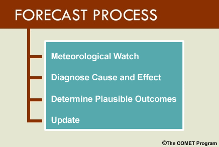
Our Forecast Process image below shows that this lesson involves all parts of the forecast process we’ve been discussing.
In this lesson, we will show how all the skills and tools you have studied so far can be used to add value to the NWP guidance. At the end of this lesson you will be able to:
- Determine when and where you can add value by comparing your conceptual model to the NWP forecast
- Evaluate the ability of NWP models to predict meteorological features expected to impact your area at the short and medium forecast range
Where are opportunities to add value to NWP output to make the best possible forecast? We will begin by examining the strengths that an individual forecaster’s experience brings to the process of forecasting. Then we’ll discuss NWP model physics and how they can limit the model’s ability to forecast certain phenomena. Next, we’ll describe how diagnostic and analytical tools can also help us assess the quality of NWP model guidance. We’ll discuss verification in real-time and use it to identify potential areas of improvement.
We highly recommend that you complete the previous sections of this NWP course before studying this lesson.
Human Experience and Pattern Recognition
Question
What enables human forecasters to improve on NWP guidance? (Choose the best answer.)
The correct answer is a).
Experienced forecasters have an ability to recognize unfolding weather patterns in a way that computers running mathematical models cannot. Choice b) is incorrect because the human cannot determine precisely how convection will develop, including timing, location, or convective mode, before it actually begins to develop. We are still unable to identify the large-scale impacts of minor errors, thus, c) is incorrect. Finally, d) is incorrect because the human is, with the possible exception of the large scale, unable to accurately imagine the evolution of the atmosphere beyond the short range.
The expert forecaster’s ability to identify weather patterns comes from long experience interpreting “fine sets of cues” that occur during a weather event. This was discussed in a 2003 research study on cognitive task analysis which investigated the weather expertise specific to warning forecasts (Klein Associates, Inc. for the Office of Climate, Water, and Weather Services in Norman Oklahoma). They found that in this area of forecasting, “The process often starts when they [forecasters] get up in the morning and look out the window” and continues at work “… when they realize which part of the weather front or which cell needs special attention. The expertise plays in specifically when the forecaster looks at the squall line and is able, based on his experience and mental model, to make specific predictions as to which part of the line will accelerate and where it will turn and cause damage. It is the fine set of cues that speak to the large amount of experience of the expert that allows the forecaster to make a warning decision for a specific area before the actual event is happening.” (Hahn, Rall, and Klinger, 2003)
The forecaster’s conceptual models and their ability to recognize patterns play a significant role even in forecasting difficult-to-predict phenomena such as severe convection. Hahn, Rall, and Klinger concluded that: “Experts have developed mental models that allow them to play out the individual scenarios and recognize patterns that novices are often not sensitized to. It is this expertise of knowing when severe is severe enough, recognizing the nuances of the storm’s development even in face of irregularities that allows experts to make warning decisions to keep the public informed ahead of the storm.” (Hahn, Rall, and Klinger, 2003)
Our ability to integrate observations and model data into a conceptual model of the atmosphere enables us to recognize the unfolding processes. In turn, we can identify patterns and anticipate the development of short-term weather events. For example, when there is strong westerly low-level flow over and east of the Appalachians, we can increase short-range model maximum temperatures in the downwind regions. NWP models do not sufficiently mix out the boundary layer to reflect this compressional warming. At the medium range, when there is a long-wave trough in the central U.S., arctic air often will move further south out of Canada than the NWP models indicate. We can identify this pattern and improve on the model output in the affected areas.
Since this study, convection-allowing models have become operational at the Storm Prediction Center and are used to anticipate types of convection and the possibility of tornadoes. Human forecasters continue to be effective, however, in improving forecast accuracy in the short range time frame. The next section will examine model limitations that enable human forecasters to improve NWP guidance.
Model Physics and Other Model Limitations
In the NWP Basics and Background course, we learned about the influence of model physics on NWP forecasts:
“The influence of model physics on the forecast of sensible weather varies significantly depending upon the meteorological situation. In general, its influence is:
- Important when dynamic forcing is weak or when physical processes are strong, such as near the center of a high-pressure system or during a clear, calm night.
- Reduced when dynamic forcing is strong, such as during a frontal passage or near a developing low-pressure system.”
Model physics impact the forecast through the parameterization of grid-scale precipitation, convection, vegetation processes, soil moisture, surface snow pack, radiation and its interaction with both clouds and the surface, and more. To learn more about model physics and parameterizations visit the lesson, Influence of Model Physics on NWP Forecasts - Version 2 and the parameterizations discussed there. Examples there show the impact of errors in each of these physics elements on the forecast.
Tools Which Can Be Used to Add Value to NWP Output
We have discussed the use of diagnostic, post-processing, probabilistic and other tools in the forecast process in previous lessons. The table below lists the tools covered in this course, organized by forecast process step. This is not an exhaustive list; new tools are being developed in the WFOs by creative and innovative forecasters.
|
Forecast Process Step |
Tool |
| Meteorological Watch (Lesson 2) |
|
| Diagnosing Cause and Effect (Lessons 3, 4, and 5) |
|
| Determining Probable Outcomes (Lessons 4 and 6) |
|
| Update (Lesson 3) |
|
Refer to the individual lessons for information on how to apply these tools in the forecast process.
One tool not in the list is MOS guidance. Since it is bias-corrected, systematic errors from the model have been removed and MOS guidance makes for a good starting point. As you incorporate MOS guidance in your forecast process, the following considerations will enable you to add value to it:
- Are the environmental conditions typical or atypical; that is, are events occurring as one would normally expect? A "typical" sample set leads to a good forecast.
- Are the MOS parameters derived separately for each station (such as temperature), or are they developed together for a region due to small numbers of events? You need to know whether the parameters of interest have regional equations, and if so, how the station of interest tends to differ from others in the region under the same large-scale conditions.
- Data sets are stratified seasonally. Most forecast variables have cool season equations from October 1 through March 31 and warm season equations from April 1 through September 30. See the MOS FAQ for specifics.
- MOS performs better than raw model forecasts where local factors may have influenced the forecast too little or too much. See Bias correction in MOS.
- For more information visit: The MOS Technique: General Information and COMET lesson Intelligent Use of Model-Derived Products.
Verification
One tool not discussed in this course is verification. Verification helps us improve our performance and fine-tune our understanding of how numerical models depict atmospheric features. The latter is crucial for developing conceptual models of the atmosphere and helping us apply this knowledge to the forecast process.
Let’s review the table below. It shows the maximum temperature verification (bias) of the first five periods for a hypothetical location A. The NAM MOS (MET), GFS MOS (MAV), NDFD Grids (Human), and GFS raw forecast (GFS) are included in the comparison.
|
PERIOD |
MET |
MAV |
Human Forecaster |
GFS |
| 1 | -0.1 | 0.0 | 0.6 | 0.1 |
| 2 | -0.7 | -0.2 | 1.9 | 0.2 |
| 3 | -0.7 | 0.0 | 1.0 | -0.7 |
| 4 | 0.2 | 0.3 | 1.8 | 0.8 |
| 5 | -1.3 | -0.3 | -2.7 | -1.0 |
| MEAN BIAS | -0.52 | -0.04 | 0.52 | -0.12 |
Question
In the table above, which is the verification score with the greatest variation? (Choose the best answer.)
The correct answer is c).
The human forecaster has the greatest variance in forecast errors, with a warm bias overall (except for period 5, which has a large cool bias). We see that in this particular case, the MAV has the best score each period and overall for the full forecast. The MET has a fairly consistent cool bias, and the GFS varies from cool to warm bias from period to period.
This verification table points to a learning opportunity for the human forecaster. The forecaster needs to review the forecasts for these periods (including their own), determine the reasons for these biases, and adjust his/her conceptual models to correct for them in the future.
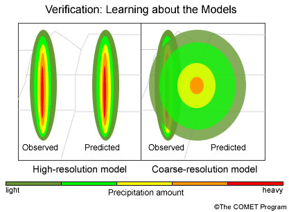
Some verification methods are more useful for some meteorological variables than others. In the image below we see a forecast for a narrow, heavy rain band. On the left, we have a high resolution model that does a good job of predicting the shape and the intensity of a precipitation band, though it is displaced to the east. Because of the displacement, this model will have a low verification score. In contrast, on the right, we have a coarse resolution model which gets the shape and intensity incorrect but includes some of the area where rain actually occurred. Because of the overlap in forecast and observed precipitation, this forecast would get a higher score, though it is no better than the high-resolution forecast. The forecaster can use this information to better understand how the models represent precipitation, so that if a similar situation arises in the future, the forecaster can incorporate this understanding into their conceptual model and generate a more precise precipitation forecast. For example, the forecaster could use the shape of precipitation in the high-resolution model and apply it to the location where s/he believes the precipitation will actually take place.
Discussion of appropriate verification for these variables is beyond the scope of this course. For further discussion on these issues, see Baldwin and Kain (2006) and the series of articles beginning with Gilleland, et al. (2009) evaluating a wide variety of new verification approaches specifically designed to address this difficulty.
Case Study One
The following case study presents a weather situation from North Texas and the Dallas-Fort Worth county warning area (CWA) for 10 August 2010. Below is a synopsis of the weather in the days leading up to 10 August.
Synopsis:
In late July and early August 2010, the southern part of the U.S. from the Carolinas to New Mexico was experiencing warmer than normal temperatures. High pressure both at the surface and aloft extended westward from the Atlantic over this area. In this flow pattern, the Dallas-Fort Worth CWA was experiencing an extended period of maximum temperatures at or exceeding 100ºF and low temperatures between 75 and 82ºF, with the warmer minimums in urbanized areas. Dewpoints throughout the area were in the upper 60s to low 70s °F.
You are the day shift forecaster on duty during 10 August 2010. We have the following animation of 500-hPa height analyses at 24-hour intervals for the last 4 days, ending 00 UTC 10 August. After examining the animation, answer the question below.
Question
What is the most persistent weather feature in the animation above affecting the Dallas-Fort Worth CWA? (Choose the best answer.)
The correct answer is b).
In all the analyses, the deep high pressure system continued to dominate the area, as can be seen in the animation from 00 UTC 7 August through 00 UTC 10 August. The flow is fairly amplified for summer, so a) is incorrect. Choice c) is incorrect because any short waves are well to the north of Texas, as is typical for summer.
Past Model Performance
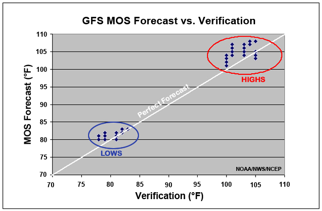
A scatter plot showing GFS MOS forecasts versus the verification for maximum and minimum temperature for Dallas-Fort Worth Airport (KDFW) is shown below. Forecasts are for all cycles from 5 through 9 August. Repeated forecast/verification pairs are plotted on top of each other. The white diagonal marks perfect forecasts, and the maximum and minimum temperatures are annotated (HIGHS and LOWS inside the red and blue circles, respectively).
Question
Based on the information in the graphic above, what can you say about the performance of the GFS MOS during the past flow regime?(Choose the best answer.)
The correct answer is c).
There is a forecast warm bias on average; only three maxima verified warmer than the forecast, and only one minimum did so, so responses a) and b) are incorrect. In fact, every daily cycle (00, 06, 12, and 18 UTC) exhibited very similar biases in both maximum and minimum temperature forecasts.
Current GFS 12 UTC 10 August 2010 Forecast
We show below, an animation of the GFS 12 UTC 10 August 2010 Forecast of 500-hPa heights at 24 hour intervals through day 4. While we do not show convective available potential energy (CAPE) and convective inhibition (CIN) over the forecast period, the GFS 12 UTC 10 August run does show that there is some CAPE available for convection, but also enough CIN to suppress convective scheme triggering in the GFS. Sea level pressure in the southern Plains gradually lowers during the period, with the 1000-500 hPa thickness remaining at or above 585-dm. After you have examined the animation below and considered the additional information above, please answer the question below the graphic.
Question 1
Based on the synopsis and the data you have seen on the previous pages, which of the following conceptual models would you adopt? (Choose the best answer.)
The correct answer is b).
A cursory examination of the forecast flow pattern at 500-hPa from the 12 UTC 10 August 2010 GFS shows no significant changes for the next 4 days. The synopsis and current observations indicate that conditions are not expected to change. Answers a), c), and d) indicate changing conditions in the near future to varying degrees, which do not agree with the expected outcome.
Question 2
Which of the following area forecast discussions (AFDs) describe the actions that would make the best use of your time in developing the forecast for the next four days? (Select all that apply.) Note that only the pertinent portion of the AFD is presented here.
Both b) and c) are potentially correct.
Recent verification indicated that the GFS MOS guidance had warm biases during this weather regime, which is expected to continue. Depending on your confidence in the GFS MOS guidance, a forecast of persistence for low and high temperatures or an adjustment to the forecast could work well. Your level of experience with atmospheric patterns in this forecast area will determine which approach you take.
This case is an example of a situation in which the forecaster can use persistence as a forecast when conditions are expected to remain constant over a period. The forecaster’s conceptual model of the atmosphere indicates that conditions are likely to persist in the day 1 through 4 period. This enables the forecaster to spend her/his time wisely and avoid wasting hours on analysis, to make what would amount to a minor adjustment to forecast grids. It also shows how verification can be helpful in making a forecast decision.
Case Study Two
Assume that you just started working the evening shift around 2:30 PM CST and are interested only in near term forecasts that do not extend beyond midnight CST.
Synopsis:
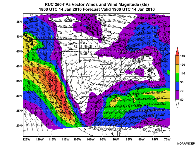
On the afternoon of 14 January 2010 a surface low pressure system formed across northern Mexico. This system was unusual because the jet stream associated with it was much farther south than normal, over Southern Mexico, as can be seen in the graphic below. There also is a strong jet streak with winds in excess of 150kt, upwind of an upper-level trough over northwest and western Mexico.
Let’s review the following case study involving precipitation in the near term. Assume that you just started working the evening shift around 2:30 PM CST and are interested only in near term forecasts that do not extend beyond midnight CST.
Current Observations
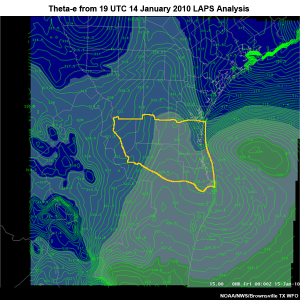
Studies (e.g. Hane et al., 2001) have shown that moisture gradients can support the development of thunderstorms given the proper larger-scale environment. Below is a graphic from 19 UTC 14 January 2010 from the Local Analysis and Prediction System (LAPS) analysis over south Texas.
At this time, we have 925-hPa and 850-hPa convergence of about 2-3 x 10⁻⁵ per second and divergence above 700-hPa. CAPE is about 900-1000 JKg-1, and CIN is less than -50 JKg-1 over and around the forecast area.
Question
Given the data in the graphic below, in what area would you be looking for convection over the next few hours in the Brownsville, TX CWA? (Choose the best answer.)
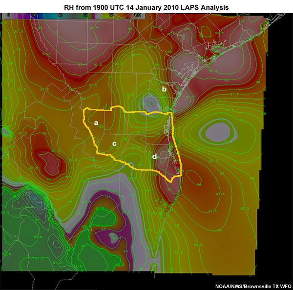
The correct answer is d).
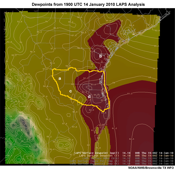
There is a 20% relative humidity gradient across the north-easternmost tip of Mexico and across the Brownsville TX CWA. This is the area that would be prime for thunderstorm development given that there is a moderate amount of CAPE with little or no CIN. There also is a 5°F dewpoint gradient across the area, as shown in the LAPS analysis of dewpoints below. This supports watching for thunderstorm development over Location "d". Location "b", in the Corpus Christi TX CWA, is also favorable for potential thunderstorms, but is outside the Brownsville CWA.
NWP and HPC Guidance
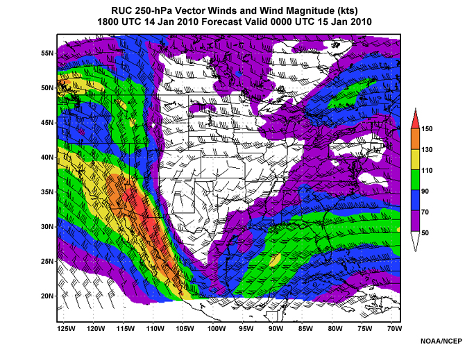
Between 19 UTC 14 January and 00 UTC 15 January 2010, the strong jet streak was forecast to shift slightly eastward and southward, and 250-hPa winds were to increase by about 20kt over deep south Texas. Note the closed upper-level low over west Texas, and the negatively-tilted upper-level trough extending from that low to northeast Mexico. There is a tendency toward diffluence east of this trough, including over south Texas.
At 12 UTC on the 14th, the Hydrological Prediction Center (HPC) issued the following accumulated precipitation forecast for the 06-hr period ending at 00 UTC 15 January 2010. It showed general precipitation coverage of up to one-third inch in 6 hours in south TX.
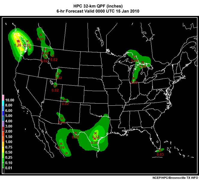
In addition, recall that there is lower tropospheric convergence and mid- to upper-tropospheric divergence in south Texas, along with a moderate amout of CAPE. You also note that winds are southeasterly at the surface and 850-hPa, southerly at 700-hPa, and southwesterly at 500 and 400-hPa. These conditions are forecast to persist through at least 06 UTC 15 January 2010 (except with convection, instability would obviously decrease). A surface trough extending northeast from north-central Mexico lies on the Gulf coast of deep south Texas at 21 UTC 14 January 2010. This trough is forecast to remain in place over the next 6-12 hours as low pressure is forecast to shift eastward to the northern Gulf coast of Mexico.
Question 1
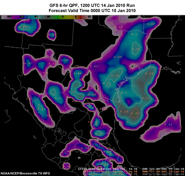
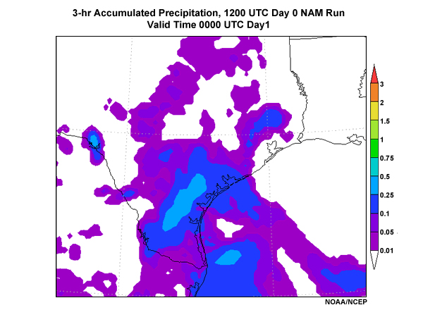
Below are accumulated precipitation graphics for the 6-hour period ending 00 UTC 15 January 2010 from the 18 UTC GFS, the 3-hour period ending 00 UTC 15 January 2010 for the NAM, and for the 3-hour period ending 23 UTC 14 January 2010 from the 20 UTC RUC. This can be considered a poor man’s ensemble (See Determining Plausible Forecast Outcomes).
GFS
NAM
RUC
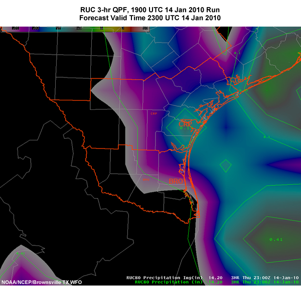
What can you conclude about the location of precipitation from the three model forecasts? (Choose the best answer.)
The correct answer is c).
There is some discrepancy among the models regarding the coverage and geographical location of the precipitation for the evening. The 18 UTC GFS, as well as previous runs (not shown), showed a broad area of precipitation mainly covering the central and eastern portions of Deep South Texas. A similar solution is forecast by the 12 UTC NAM with higher QPF values over the northern portions of Deep South Texas. The ECMWF (not shown) was very similar in coverage and character to the GFS. The RUC model maintained most of the precipitation out to sea, including the 12 hr forecasts starting around 12 UTC on 14 January (not shown). The 3 hour RUC forecast valid at 23 UTC, however, showed more coverage of forecast precipitation over land compared to prior runs.
Question 2
Based on the observations and forecast guidance, which of the following conceptual models would you adopt over the period from now through 06 UTC 15 January 2010? (Choose the best answer.)
The correct answer is c).
While model guidance indicates light to moderate
precipitation amounts will occur over the CWA, observations and the short-range
forecast for stability parameters indicate potential for convection along
existing moisture gradients. Such convection would further focus moisture
convergence and increase rain rates where it occurs. This conceptual model helps
the forecaster focus his/her attention in areas where the forecast models may
not perform so well.
For answer a), the model and HPC guidance does
indeed indicate this general scenario. The model guidance, however, often does
not handle the triggering and movement of convection well. If convection occurs,
this guidance will give a poor forecast.
For answer b), high
relative humidity alone does not determine where precipitation will occur. In
the case of convection, model forecasts do not help us in identifying where and
when thunderstorms will take place.
Below is a graphic of the equivalent potential temperature from the 00 UTC 15 January 2010 LAPS analysis. In addition to this graphic, forecast data indicates that precipitable water values will increase from 2.5-3 cm to 3-3.5 cm (1-1.2 inches to 1.2-1.4 inches) between 00 UTC and 06 UTC 15 January 2010. Winds will continue from the south to southeast at levels at or below 700-hPa and from the southwest above that level. Finally, CAPE is expected to remain at about 800-1000 JKg-1.
Question 3
Based on this information, what weather processes could happen after 00 UTC? (Choose the statement that best describes the potential outcome.)
The correct answer is a).
To see whether the environment is favorable for the continuation of any convection that might develop, we can look at the amount of instability available at and downwind of its potential location. In the figure, we see a tongue of higher values of equivalent potential temperature around the possible thunderstorm development area from the LAPS analysis. Additionally, even higher values of equivalent potential temperature are offshore, and will be advected into the northern part of the CWA by the prevailing easterly surface winds. This should support any thunderstorms as they move or redevelop into the northeastern part of the CWA, steered by the prevailing winds from the southeast to south in the lower troposphere, and from the southwest in the middle- to upper troposphere.
Question 4
Based on the observations, forecast guidance, and the conceptual model of the current state of the atmosphere, what precipitation forecast would you make for the period from now through 06 UTC 15 January 2010? (Choose the best answer.)
The correct answer is a).
We expect convection to develop in the moisture gradient from
near Brownsville northwestward into the center of the CWA. The moist, unstable
air to the north and east of this region would support the propagation and
maintenance of this convection. Item b) and c) are not the best choices because
of the risk of thunderstorms in the area, resulting from the horizontal moisture
gradients near the coast and the moderate instability as represented by the
800-1000 J Kg-1 CAPE values.
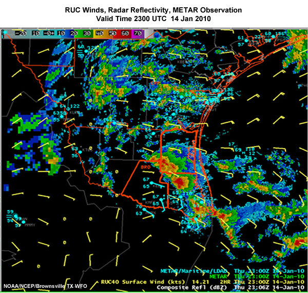
To support this conclusion,
below is a graphic of radar reflectivity with RUC winds and METARs superimposed
from 23 UTC 14 January 2010.
Case Study Two: Summary
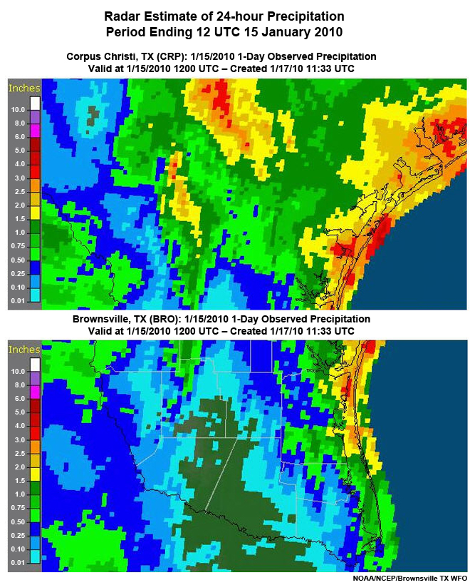
Below is the estimated radar precipitation for the Brownsville and Corpus Christi CWAs. Without the convection, perhaps the 0.1 - 0.25" precipitation amounts in the NWP model forecasts and HPC guidance would have been accurate. With the thunderstorms and the enhanced moisture convergence, however, the rain rates increased significantly. This resulted in rainfall amounts of 0.5 to 3" for the 24 hour period ending 12 UTC 15 January 2010. The available NWP models could not properly simulate the thunderstorms, which presented an opportunity for the forecaster. By using the continuous meteorological watch, s/he could have enhanced model forecast precipitation to reflect the presence, expected movement, and continuation of convection.
Summary
This lesson discussed how we can recognize where and when the human can add value to NWP guidance. We reviewed the forecast processes elaborated in the course and reflected on the role of human experience in the process. Our ability to recognize patterns and develop conceptual models plays a significant role even with difficult-to-predict phenomena such as convection.
We then reviewed the tools available to the forecaster to assist him/her in the four steps of the forecast process. Then, we discussed the role of verification in helping us improve our performance and fine tune our understanding of how numerical models depict atmospheric features. This may help us determine the effect of limitations in model physics on forecast guidance.
Finally, we examined two cases where the forecaster could add value to NWP guidance. In the first case, the forecaster could have used persistence as a forecast because conditions were expected to remain constant over a period. The forecaster’s conceptual model of the atmosphere indicated that conditions were likely to persist. This enabled the forecaster to spend their time wisely and avoid wasting hours on analysis, to make what would amount to a minor adjustment to forecast grids. The case also showed how verification could be helpful in making a forecast decision.
The second case illustrated the use of the continuous MetWatch to identify departures of the real atmosphere from the model forecast, and to make appropriate adjustments. The departure in this case resulted from the inability of the models to accurately predict timing and location of convection. This inability was due to limitations of the convective parameterizations in these models.
Careful implementation of the steps of the forecast process outlined in the course will help you identify opportunities to add value to NWP guidance. As we have seen in this lesson, some situations may call for using persistence and not investing large amounts of time into analysis. Others require careful analysis of the current and expected conditions and the model guidance, to determine the most likely forecast scenario. Your experience as a forecaster is important in determining when and where to add value.
References
Hane, Carl E., Michael E. Baldwin, Howard B. Bluestein, Todd M. Crawford, Robert M. Rabin, 2001: A Case Study of Severe Storm Development along a Dryline within a Synoptically Active Environment. Part I: Dryline Motion and an Eta Model Forecast . Mon. Wea. Rev., 129, 2183-2204.
Ahijevych, D., E. Gilleland, B.G. Brown, and E.E. Ebert, 2009: Application of spatial verification methods to idealized and NWP-gridded precipitation forecasts. Wea. Forecasting, 24, 1485–1497
Baldwin, M.E., and J.S. Kain, 2006: Sensitivity of several performance measures to displacement error, bias, and event frequency. Wea. Forecasting, 21, 636–648
Casati, B., 2010: New developments of the Intensity-Scale Technique within the Spatial Verification Methods Intercomparison Project. Wea. Forecasting, 25, 113–143
Coniglio, M.C., K.L. Elmore, J.S. Kain, S.J. Weiss, M. Xue, and M.L. Weisman, 2010: Evaluation of WRF model output for severe-weather forecasting from the 2008 NOAA Hazardous Weather Testbed Spring Experiment. Wea. Forecasting, in press
Gilleland, E., D. Ahijevych, B.G. Brown, B. Casati, and E.E. Ebert, 2009: Intercomparison of spatial forecast verification methods. Wea. Forecasting, 24, 1416–1430
Lack, S.A., G.L. Limpert, and N.I. Fox, 2010: An object-oriented multiscale verification scheme. Wea. Forecasting, 25, 79–92
Marzban, C., and S. Sandgathe, 2009: Verification with variograms. Wea. Forecasting, 24, 1102–1120.
Rife, D.L., C.A. Davis, Y. Liu, and T.T. Warner, 2004: Predictability of low-level winds by mesoscale meteorological models. Mon. Wea. Rev., 132, 2553–2569
The National Weather Service Office of Climate, Water, and Weather Services, cited 2010: Cognitive Task Analysis of the Warning Forecaster Task. [Available on line at http://www.wdtb.noaa.gov/modules/CTA/index.html]
Contributors
COMET Sponsors
The COMET® Program is sponsored by NOAA National Weather Service (NWS), with additional funding by:
- Air Force Weather (AFW)
- European Organisation for the Exploitation of Meteorological Satellites (EUMETSAT)
- Meteorological Service of Canada (MSC)
- National Environmental Education Foundation (NEEF)
- National Polar-orbiting Operational Environmental Satellite System (NPOESS)
- NOAA National Environmental Satellite, Data and Information Service (NESDIS)
- Naval Meteorology and Oceanography Command (NMOC)
Project Contributors
Project Lead
- Dr. William Bua— UCAR/COMET
Instructional Design
- Tsvetomir Ross-Lazarov — UCAR/COMET
Principal Science Advisors
- Dr. Jeral Estupiñán — NWS WFO Miami FL
Graphics/Interface DesignEr
- Brannan McGill — UCAR/COMET
Multimedia Authoring
- Carl Whitehurst — UCAR/COMET
Senior Project Manager
- Dr. Greg Byrd — UCAR/COMET
COMET HTML Integration Team 2020
- Tim Alberta — Project Manager
- Dolores Kiessling — Project Lead
- Steve Deyo — Graphic Artist
- Gary Pacheco — Lead Web Developer
- Justin Richling — Web Developer
- David Russi — Translations
- Gretchen Throop Williams — Web Developer
- Tyler Winstead — Web Developer
COMET Staff, Fall 2010
Director
- Dr. Timothy Spangler
Deputy Director
- Dr. Joe Lamos
Administration
- Elizabeth Lessard, Administration and Business Manager
- Lorrie Alberta
- Michelle Harrison
- Hildy Kane
- Ellen Martinez
Hardware/Software Support and Programming
- Tim Alberta, Group Manager
- Bob Bubon
- James Hamm
- Ken Kim
- Mark Mulholland
- Victor Taberski - Student Assistant
- Chris Webber - Student Assistant
- Malte Winkler
Instructional Designers
- Dr. Patrick Parrish, Senior Project Manager
- Dr. Alan Bol
- Maria Frostic
- Lon Goldstein
- Bryan Guarente
- Dr. Vickie Johnson
- Tsvetomir Ross-Lazarov
- Marianne Weingroff
Media Production Group
- Bruce Muller, Group Manager
- Steve Deyo
- Seth Lamos
- Brannan McGill
- Dan Riter
- Carl Whitehurst
Meteorologists/Scientists
- Dr. Greg Byrd, Senior Project Manager
- Wendy Schreiber-Abshire, Senior Project Manager
- Dr. William Bua
- Patrick Dills
- Dr. Stephen Jascourt
- Matthew Kelsch
- Dolores Kiessling
- Dr. J. Cody Kirkpatrick
- Dr. Arlene Laing
- Dave Linder
- Dr. Elizabeth Mulvihill Page
- Amy Stevermer
- Warren Rodie
Science Writer
- Jennifer Frazer
Spanish Translations
- David Russi
NOAA/National Weather Service - Forecast Decision Training Branch
- Anthony Mostek, Branch Chief
- Dr. Richard Koehler, Hydrology Training Lead
- Brian Motta, IFPS Training
- Dr. Robert Rozumalski, SOO Science and Training Resource (SOO/STRC) Coordinator
- Ross Van Til, Meteorologist
- Shannon White, AWIPS Training
Meteorological Service of Canada Visiting Meteorologists
- Phil Chadwick