Print Version
Table of Contents
Introduction
Bias in numerical weather prediction (NWP) models is nothing new to forecasters, who often hear statements like:
"The NAM (North American Mesoscale model, also known as WRF-NMM) has too little convective precipitation during the western U.S. summer monsoon season" or "The GFS (Global Forecast System) always has a cold bias in the lower troposphere during winter".
Until recently, there were no objective bias-corrected NWP forecasts from the U.S. national centers. That changed in the mid 2000s with the development of bias-corrected probabilistic precipitation forecasts from the NCEP global ensemble forecast system (GEFS). Subsequently, bias-corrected data became available from the NCEP deterministic Global Forecast System (GFS), the North American Ensemble Forecast System (NAEFS) and the Short-Range Ensemble Forecast (SREF) system. While these data are not pushed directly into the NWS's Weather Forecast Office (WFO) AWIPS, some WFOs pull in the data for use in the forecast process.
Now that bias-corrected forecasts can be accessed by WFOs, it behooves forecasters to become familiar with these products and their advantages and limitations.
After completing this module you will be able to:
- List three forecast situations in which bias correction is useful.
- List three tools that are used to bias-correct the forecast.
- Identify some of the advantages and limitations of each tool.
- Use bias-corrected data effectively in a medium range forecast.
- Use bias-corrected data effectively in a 1-2 day (short range) forecast.
What Is Bias?
Let's say you throw 100 baseballs, aiming at the same spot each time. You won't likely hit the same spot each time. There may be a flaw in your throw so you hit high and to the right of the target. There will also be errors beyond your control like random variation in the wind, an imperfect ball, or other complications. These are two different kinds of errors. One you can correct, while the other you cannot. The flaw in your throwing style can be corrected with practice and is known as a bias. The errors from random variation in wind and imperfections in the ball are not correctable and are known as random errors. The bias and the random error together constitute the total error. In NWP models, both random errors and bias can and do occur on a regular basis. How we determine what biases can be corrected is the subject of the rest of this module.
When Do You Use Bias Correction?
The most important decision for you to make about bias-corrected data is when to use it. There are three types of situations where you, the forecaster, can add value to a forecast by using bias-corrected data:
- a situation where a long-term regime will remain in place (regime continuity)
- a situation where correcting will remove some of the bias from a forecast timing issue (timing)
- a situation where correcting will remove some of the bias from a forecasted event in a model that didn't occur in reality or vice versa (existence/limitation).
We can explain these three types of situations using our baseball example from above.
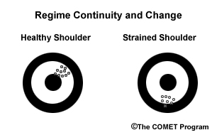
Regime continuity: You are trying to throw 100 baseballs at a target. If nothing irregular happens to your throwing arm, you will likely maintain the same bias (high and right of center). Bias correction would be useful at this time to correct your miscue. If you strained your shoulder 50 throws into your series, then your bias will likely change, and the same bias correction scheme would no longer work. The former situation is an example of regime continuity, while the latter is an example of regime change. Since you did not injure your shoulder in the first 50 throws, there was no change in your throwing bias so your throwing regime was maintained. After you strained your shoulder, there was a change in your throwing bias. Because of your injury the regime has changed.
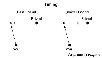
Timing: You are again trying to throw 100 baseballs at a target, but this time the target is moving, a friend running right-to-left in front of you. If your friend runs at the same speed every time, then you can correct your high and right bias to always predict where to throw the ball so she can catch it. Bias correction will increase your accuracy. After 50 throws, your friend is tiring and begins to slow her pace. When this occurs, the same bias correction would no longer work because you will throw to her previously predicted location using her faster speed. The former situation is an example of when the timing of the predicted event was appropriately corrected, while the latter is an example of inappropriately correcting for timing of an event.
Existence/Limitation: You are trying to throw 100 baseballs to your stationary friend with your eyes closed. Your friend can place herself anywhere around you but must remain the same distance away from you. You must choose the location to throw all 100 balls. It is unlikely that you will throw the balls to your friend's location. After you open your eyes, you can note your bias and figure out how to correct for it, thus increasing your accuracy.
Let's examine a few examples of these biases in meteorological data.
Regime Continuity
In all of the previous analogies, the thrower can be the forecaster, the ball is the NWP forecast, and the target or friend would be the verification. Here are some examples of the three types of situations where bias correction increases forecast accuracy.
When you were throwing the ball at the stationary target in the examples above, that was a regime-continuity issue that could be bias-corrected. In meteorological data, regime-continuity issues are often encountered with extended periods of the same weather pattern (no shoulder injury). Below we show examples of regime continuity where a biased model forecasts a continuation of the same weather pattern. These are situations when bias-correction will usually result in a better forecast than using raw model data:
- Your area has been in a cold weather regime resulting from being near a long wave trough axis over an extended period in the winter season
- Your area has been wetter than normal because of a displacement of the normal storm track from normal and the impact of the resulting wet soils for a couple of months during the warm season
Question
You're under a deep-layered ridge of high pressure in the center of the CONUS during the warm season. This ridge is expected to remain in place. The models have been showing a cold bias in near-surface temperature during this particular flow regime. Would it be helpful to use a bias-corrected forecast in these circumstances? (Choose the best answer.)
The correct answer is a.
Because the forecast problem of the day has remained consistent throughout the period, correcting a bias will increase forecast accuracy. Using the bias-corrected forecast would yield the best forecast.
On the other hand, below are examples of regime change where a biased model forecasts a change in the weather pattern. These are situations when bias-correction will usually result in a worse forecast than using raw model data, because the former flow regime bias may no longer apply:
- After being under a blocking ridge, a shift in the flow puts your area in the vicinity of a long-wave trough
- After a long-term drought, your area experiences flooding rains.
Question
After an extended period with unseasonably persistent snow cover in the cold season and a persistent warm bias in 2-m temperatures, a warm spell quickly melts the snow. Would it be helpful to use a bias-corrected forecast in these circumstances? (Choose the best answer.)
The correct answer is b.
The unseasonably persistent snow cover in itself can be considered a type of regime. Additionally, the persistence of the snow cover indicates a persistent flow regime. The removal of the snow will change the weather regime by itself, but the warm spell that melted the snow signals a change in flow regime as well. The change of regime will result in bias-corrected forecasts performing worse than raw forecasts, until the new regime is incorporated into the bias that is being corrected for.
Timing
When you were throwing the ball to your moving friend in the examples above, that was a timing issue that could be bias-corrected. In meteorological data, timing issues are often encountered with frontal passages, cloud advection, and cyclone or anticyclone arrival times. Examples of when you'd expect the bias-corrected forecast to perform better than a raw forecast include but aren't limited to, the following situations:
- You expect a warm front to cross your area later than forecast, and a warm bias is being removed
- You expect a cold front to cross your area later than forecast, and a cold bias is being removed
Examples of when you'd be able to add value to an erroneous bias-corrected forecast would include but aren't limited to, these situations:
- You expect a warm front to cross your area earlier than forecast, and a warm bias is being removed
- You expect a cold front to cross your area earlier than forecast, and a cold bias is being removed
Below we show an example of a frontal timing issue where the model forecasts the front to pass later than in reality.

Forecast versus verification of frontal position for a hypothetical example of an arctic front advancing eastward across the Midwest. Forecast cold front is in light blue. Verification cold front in dark blue with cold front barbs pointing in direction of frontal movement. Forecast area of interest, Davenport IA area, is marked with a bold, black X. Note label for Arctic air mass over the northern High Plains.
Question 1 of 3
If you were a forecaster in Davenport, IA (shown with an "X") forecasting the 2-m temperature, would it be useful to bias-correct your forecast based on the above graphic? (Choose the best answer.)
The correct answer is c.
You would need to know how the bias correction would affect the forecast temperature (warms or cools) to determine whether to correct or not in any forecast scenario. a) is very tempting because we know there is a forecast discrepancy, however, one needs to know how the forecast will be altered by the bias correction (warmed or cooled). b) is incorrect. Even though it may be true that bias correction may not be necessary, you do not have enough information to make this decision yet.
Existence
When you were throwing the ball with your eyes closed, that was an existence issue that could be bias-corrected. In meteorological data, existence issues occur when a model produces an event that does not occur in reality or the opposite - a model does not produce an event that actually occurs. Examples where bias-correction would improve the forecast as a result of an existence or non-existence issue would include situations where:
- A cold bias is being removed, and model cloudiness from overrunning is erroneously forecast in your area during daylight hours.
- A warm bias is being removed, and model cloudiness from overrunning is erroneously forecast in your area overnight.
- A dry bias is being removed, and significant rainfall occurs that is missed by the forecast model.
Examples where bias-correction would degrade the forecast would include:
- A warm bias is being removed, and a model snowfall does not materialize.
- A cold bias is being removed, and model cloudiness from overrunning is erroneously forecast in your area overnight.
- A cold bias is being removed, and an unpredicted warm-season mesoscale convective system (MCS) cloud shield moves over your area during daylight hours.
IMPORTANT NOTE: The average model bias is usually small, particularly in regions with relatively flat topography. In such areas for example, 2-m temperature bias is usually only a degree or two Fahrenheit even at long lead times. Therefore, if either timing or existence errors are of high impact to the forecast in these regions, the forecaster can significantly improve either the raw or bias-corrected forecast. We have an example of such a forecast later in the lesson.
Below we ask a question about an existence issue where the model forecasts an event that does not occur in reality at the location of interest.
Question 1 of 3
Below we show an example of a frontal timing issue where the model forecasts the front to pass later than in reality.
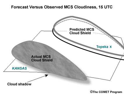
Here is an idealized graphic depicting a forecast MCS cloud shield at 15 UTC on a summer day, contoured in gray and black (shadow) in a forecast model that results from a convective "bulls-eye" upstream of Topeka, Kansas. While an MCS actually took place, it took place farther south and west (shaded in gray and black), and the resulting cloud shield is not expected to affect Topeka. If you were a forecaster in Topeka, Kansas (shown with an "X") forecasting today's afternoon high, would it be useful to bias-correct your forecast based on the above graphic? (Choose the best answer.)
The correct answer is c.
You would need to know how the bias correction would affect the forecast temperature (warms or cools) to determine whether to correct or not in any forecast scenario. a) is incorrect because you don't know whether there is currently a warm or a cold bias being corrected. b) is incorrect. Even though it may be true that bias correction may not be necessary, you do not have enough information to make this decision yet.
Tools for Correcting Bias
As of spring 2010, there are three tools available for correcting bias in NCEP products: MOS, Decaying Average, and BOIVerify. Any of these methods would be useful for these three types of situations where bias correction would lead to a better forecast.
Model Output Statistics (MOS)
MOS removes biases by linking observed weather variables to the synoptic-scale model variables through best linear fits. Because of the linear relationships, MOS is especially good at removing representativeness biases. Examples of situations where MOS will significantly improve a model forecast include, but are not limited to:
- For 2-m temperatures:
- A valley station in a region of rugged terrain, is represented to have a higher model elevation than its actual elevation.
- A station where the land use type surrounding it is misrepresented.
- For precipitation:
- A station is in a rain shadow downwind of a mountain, but in the model is located upwind of the highest model elevation.
- A station is in an area where a sea-breeze front is climatologically likely to generate convective storms each afternoon, but the model resolution is insufficient to properly represent the sea breeze or to generate the resulting convection.
MOS also performs well when the weather regime is climatologically typical and well-sampled. Examples might include:
- A period of hot, sunny weather during June in the desert Southwest of the U.S.
- A period of dry and seasonably cold weather in North Dakota in January, with persistent snow cover.
- A period of frequent frontal passages and mostly onshore winds along the U.S. Pacific Northwest coast in the winter season.
In most commonly-observed forecast situations, MOS removes mean bias fairly well. For example, on average, MOS continues to outperform raw model forecasts of 2-m temperatures.
Every statistical method, however, has its limitations. For example, MOS cannot address regime-dependent, poorly-sampled, or intermittent errors. Meteorological examples of these limitations are:
- mislocation of lee-side cyclogenesis
- existence of snow cover in regions where it is rare
- trapping of shallow cold air masses by terrain in winter
Thorough coverage of MOS methodology can be found in the COMET module, Intelligent Use of Model-derived Products, in section Statistical Guidance, Model Output Statistics (MOS), as well as in the first portion of the Gridded MOS VISITView teletraining.
MOS Example
Here's an example of MOS performing better than the model maximum 2-m temperatures. The mid-Atlantic states were in the midst of an early spring warm spell on 7 April 2010, with a string of warm days culminating in near 90�F maximum temperatures in the Washington-Baltimore area. On the 7th, the actual maximum temperature at BWI airport turned out to be 90�F (a record high).
The graphic below shows a plot of the 1� by 1� grid-box maximum 2-m temperatures from the GFS for the 6 hours ending 00 UTC 8 April 2010. The average for the BWI grid box (marked by a black "x") is 81�F.

Forecast Maximum 2-m temperature for 6 hours ending 00 UTC 8 April 2010 from GFS 1�x1� resolution forecast. Temperatures for each grid box are printed in their centers in �Fahrenheit. Grid box including Baltimore-Washington International Airport is highlighted with vertical blue stripes. Temperatures are also contoured at 2�F intervals.
Meanwhile, the GFS MOS guidance for BWI Airport indicated the following, based on the same GFS data:
 based Model Output Statistics (MOS) forecasts, based on 00 UTC 7 April 2010 GFS model forecast data. Indicated are 24-hour maximum, 24-hour minimum, and 3-hourly instantaneous 2-m temperatures and dewpoints, cloud cover, wind direction and speed, probability of precipitation at 6 and 12 hour intervals, categorical quantitative precipitation forecast, 6-hour and 12-hour probability of thunder, probability of freezing rain and snow, most likely precipitation type, snow amount at 24 hour intervals, categorical ceiling and visibility, and what obstruction to visibility is forecast to exist, if any.")
Table of Global Forecast System (GFS) based Model Output Statistics (MOS) forecasts, based on 00 UTC 7 April 2010 GFS model forecast data. Indicated are 24-hour maximum, 24-hour minimum, and 3-hourly instantaneous 2-m temperatures and dewpoints, cloud cover, wind direction and speed, probability of precipitation at 6 and 12 hour intervals, categorical quantitative precipitation forecast, 6-hour and 12-hour probability of thunder, probability of freezing rain and snow, most likely precipitation type, snow amount at 24 hour intervals, categorical ceiling and visibility, and what obstruction to visibility is forecast to exist, if any.
Question
MOS is telling us that at this grid point the GFS typically overestimates the 2-m temperature. True or False.
The correct answer is False.
The GFS forecasted 81�F while MOS predicted 87�F which is 6 degrees warmer. This means that the GFS typically has a cold bias, or that it underestimates the temperatures at that grid point. As this is a forecast with only one day lead time, the better MOS performance is not surprising. Keep in mind that at longer lead times, MOS is more heavily weighted toward climatology. Therefore, in anomalously warm situations at long lead times, MOS would be more likely to have a cold bias.
Why did the MOS perform better? MOS performs better than raw model forecasts when local factors may have influenced the forecast too little or too much. In this case, because of the proximity of the Chesapeake Bay and relative coarseness of the GFS resolution, there is a tendency for the GFS to "alias" the bay breeze too far inland. Additional factors may have contributed to the GFS forecast error including local surface condition errors, such as:
- Soil moisture errors (here, actual soil would have to be drier than modeled)
- Vegetation greenness fraction errors (model would have to have too much greenness fraction)
- Representativeness error due to sub-grid scale variations in surface conditions not captured on a 1� x 1� grid
Now that we've covered MOS for removing some model bias, let's move on to a more recent development in bias removal involving the actual calculation of model bias in forecast variables, and its direct removal from those variables.
Decaying Average
We can use the "decaying average" method to give a greater weight to today's error relative to previous days' errors. This means that prior days will have less influence on the current bias than today does. In the graphic below, the bar heights represent the error weight for each day, showing that today has the most error weight.

Histogram of the decreasing weights assigned to total error in the calculation of decaying average as one goes back in time from the present day. The red numbers within the boxes in the histogram indicate the weight given to that day's error in percent. The boxes are scaled in size relative to the present day weighting.
The decaying average method in spring 2010 was used to produce bias-corrected data for the SREF, the GFS/GEFS, and the NAEFS at NCEP. The decaying average used in the SREF places more weight on recent errors and less on error data older than 30 days, than the GFS/GEFS and NAEFS. The weightings for the SREF and the GFS/GEFS were chosen based on the values that give the best overall results over the full forecast domain, for each system. A larger weight works better for the SREF than for the GFS/GEFS for multiple possible reasons: the smaller spatial scales in the SREF relative to the GEFS, the error characteristics of the models used in the SREF, and/or other factors. How to obtain the bias-corrected data, which is not currently pushed into the NWS Advanced Weather Interactive Processing System (AWIPS), is covered via a link in the references.
Decaying average bias correction from the model forecast results in overall improvement in model scores, thus bias-corrected products usually provide superior guidance. Below are examples where bias-corrected forecasts will perform well:
- Your area has been in a cold weather regime over an extended period in the winter season
- Your area has been wetter than normal for a couple of months during the warm season
- You expect a warm front to cross your area later than forecast, and a warm bias is being removed from the model forecast
- You expect a cold front to cross your area later than forecast, and a cold bias is being removed from the model forecast
- A cold bias is being removed from the model forecast, and model forecast cloudiness from a overrunning event is erroneously forecast to cross your forecast area.
The forecaster can add value by knowing when the bias-corrected model forecast will lead to an erroneous forecast. Below are examples where bias-corrected forecasts will perform poorly:
- After being under a blocking ridge, a shift in the flow puts your area in the vicinity of a long-wave trough
- After a long-term drought, your area experiences flooding rains.
- You expect a warm front to cross your area earlier than forecast, and a warm bias is being removed from the model forecast
- You expect a cold front to cross your area earlier than forecast, and a cold bias is being removed from the model forecast
- A warm bias is being removed from the model forecast, and today a modeled snow event has not materialized.
Remember the best results from bias correction are obtained when the bias error is a large proportion of the total error. In situations where existence and/or timing errors are large and the bias correction small, you will likely be able to improve on the NWP forecast beyond any improvement you might get from using either the bias-corrected or raw forecast!
Decaying Average Example
Below is a graphic of the day 5 forecast of 2-m temperature for the southeastern U.S. for 18 UTC on a day in mid-May. Note the below-normal temperatures expected in a band from west Tennessee east-southeastward through northern Georgia into North and South Carolina. The polygon with the red dotted shading is the forecast area of the Columbia, South Carolina office.

A plan view of a 114-hour 2-m temperature forecast in degrees Fahrenheit for the Southeast U.S. from the GFS valid 18 UTC 10 May 2010. The Columbia SC National Weather Service Forecast Office is highlighted with a red dotted polygon.
Not surprisingly, this cool area is associated with a forecast of precipitation. The 6-hour accumulated precipitation forecast valid at the same time is shown below. Overall, the precipitation and cool temperatures are collocated.

A plan view map of 114-hour, 6-hourly accumulated precipitation forecast from the Global Forecast System over the Southeast U.S. Precipitation amounts are shaded in inches at 0.01", 0.05", 0.10", 0.25" and 0.50" levels. The precipitation is forecast to occur in an overrunning band from northwest Tennessee east-southeastward into the Carolinas and Georgia. The Columbia SC National Weather Service Forecast Office is highlighted with a red dotted polygon.
The same is true for the forecast total cloud cover, shown below. The cloud cover results from warm air overrunning a dry, cool air mass. Evaporation of the forecast precipitation cools the air, while the extensive cloud cover reduces solar heating of the model surface.

A plan view of the 114-hour total cloud cover forecast in percent coverage for the Southeast U.S. from the GFS valid 18 UTC 10 May 2010. The Columbia SC National Weather Service Forecast Office is highlighted with a red dotted polygon.
Question
You are a forecaster at the Columbia, South Carolina office (marked with red-dotted polygon). You believe at day 5, overrunning will develop more slowly than forecast over the Carolinas with sunshine for the first part of the day. If you had a bias-corrected forecast available for 2-m temperature to use for your CWA, do you think it would be helpful in your forecast area? (Choose the best answer.)
The correct answer is c.
You would need to know how the bias correction affects the forecast temperature (warms or cools) to determine whether to use it in any forecast scenario. a) is incorrect because you don't know whether there is currently a warm or a cold bias being corrected. b) is incorrect because even though bias correction may not be helpful, you do not have enough information to make this decision yet.
Question
Below is the bias-correction applied to the 18 UTC temperature for the forecast date of interest. Note the extensive cool bias over all of the Southeast. Your area has about a 1.5-2.5�F cool bias.

A plan view of a 114-hour 2-m temperature forecast bias in degrees Fahrenheit for the Southeast U.S. from the GFS valid 18 UTC 10 May 2010. The Columbia SC National Weather Service Forecast Office is highlighted with a red dotted polygon.
With this information in mind, would using the bias-corrected forecast be an improvement over the raw forecast of 2-m temperature? (Choose the best answer.)
The correct answer is a.
If you expect overrunning to develop later than forecast in the model during an afternoon in May, there should be a cool bias in the 2-m temperature forecast from that model. Since the bias corrected forecast increases 2-m temperature by around 2�, using it improves the forecast. So b) is incorrect.
Verification:
Here's the GOES image valid within 15 minutes of the forecast time. We see dense cloudiness west of the Columbia, South Carolina CWA, as would be expected if overrunning was late to arrive in the area.

A plan view visible satellite map centered on Montgomery, AL for valid time 1745 UTC 10 May 2010. Image comes from UCAR's RAL lab.
The actual temperature errors verified against the GFS analysis are shown below. They were significantly larger than the bias-correction, though in the same direction. Actual surface temperatures at METAR sites were in the 60s to low 70s at 18 UTC, compared to forecast 2-m temperatures from the low 50s to near 60�F.

A plan view of the 114-hour 2-m temperature forecast error in degrees Fahrenheit for the Southeast U.S. from the GFS valid 18 UTC 10 May 2010. The Columbia SC National Weather Service Forecast Office is highlighted with a red-dotted polygon.
The bias correction in this case removed a preexisting cool bias. An erroneous daytime cloudiness and rainfall forecast in the warm season typically results in a cool bias. Therefore, using the bias-corrected forecast in this particular case adds some value to the raw forecast. The large temperature errors in this case allow the forecaster to further improve the bias-corrected forecast.
BOIVerify
Boise Verify (BOIVerify), part of the Interactive Forecast Preparation System (IFPS) software available to most WFOs, is another useful bias correction method.
BOIVerify draws a "best linear fit" to a scatter plot of forecast (NWP model or MOS) versus verification from the last 30 days for each model grid box, forecast cycle, and lead time in the grid domain. The verification can use any analyses or observational datasets rendered to the IFPS grid. The fit line maps the raw forecast into a bias-corrected forecast based on the past 30-day relationship of forecast to the gridded observations or analyses. This is shown below for 12-km resolution NAM WRF-NMM 24-hour forecast 2-m temperature data for all 00 UTC February 2009 cycles for some grid box in the Boise ID CWA.
 Grid. A best fit line has been drawn through the data in bold black. Units for forecast and verification temperatures is degrees Fahrenheit.")
A scatterplot of 12-km resolution NAM WRF-NMM 24-hour forecast 2-m temperature data for all 00 UTC February 2009 cycles versus verification, interpolated to the 5-km National Digital Guidance Database (NDGD) Grid. A best fit line has been drawn through the data in bold black. Units for forecast and verification temperatures is degrees Fahrenheit.
The bias-corrected guidance can be used in the IFPS grid (either 5-km or 2.5-km, depending on which is used by the WFO). This method breaks data down into different regimes by virtue of its regression methodology, which is an advantage of BOIVerify over MOS. There are cool and warm regimes apparent in the temperature example shown above. BOIVerify works well in regions of rugged topography, and in persistent regimes where model and observation relationships do not change significantly.
Caution should be used with BOIVerify bias-corrected data when:
- The 30-day sample may not sufficiently capture the forecast-to-verification linear relationship
- The forecast is significantly different from the range of temperature over the last 30 days
- There is large scatter around the regression line, indicating small bias and large random error
- Seasonal changes dominate flow regime relationships during transition seasons
BOIVerify Example
Here is an example of a BOIVerify plot from the Boise WFO gridded forecast editor (GFE) for the GFS-40 (i.e. GFS model data at 40-km resolution). Suppose this is the bias for the raw forecast day-2 maximum temperature for each grid box in the GFE grid, based on the BOIVerify linear regression technique. The warm and cold biases over the higher elevations are as large as �10�F. In the Snake River Basin near Boise and other population centers in Idaho, there is a warm bias of 2-5�F.

Screen capture of National Weather Service Graphical Forecast Editor using BOIVerify to downscale maximum 2-meter temperature bias errors for the uncorrected GFS at 40-km resolution to the National Forecast Guidance Database Grid. Data is for September 2006.
Question
If the general flow regime that has existed during the previous 30-days is expected to hold tomorrow, which of the following forecast grids will offer the better GFE guidance for day-2 maximum 2-m temperatures? (Choose the best answer.)
The correct answer is b.
As long as the general flow regime continues, the bias-corrected forecast grid will provide better guidance. a) is incorrect because the flow regime will remain unchanged. c) is incorrect because we know that the identified biases should continue under a persistent regime.
As we can see in the graphic below, the bias-corrected day-2 forecast error shows much smaller magnitudes than the uncorrected GFS forecast would have. The error is not completely removed because of small random errors and error in the bias resulting from only using a 30-day sample to estimate it.

Screen capture of National Weather Service Graphical Forecast Editor using BOIVerify to downscale maximum 2-meter temperature bias errors for the bias-corrected GFS at 40-km resolution to the National Forecast Guidance Database Grid. Data is for September 2006.
When and Why Does BOIVerify Help?
Because BOIVerify is effective in removing bias when a regime remains unchanged, we get a very consistent and relatively small mean absolute error once we use the bias-corrected grids. The graphics below show Mean Absolute Error (MAE) over the same 30-day period as above. The top graphic shows MAE without bias correction, while the bottom graphic shows MAE with bias correction. We see that uncorrected MAE is as high as 10�F or more, especially in rugged terrain, while the bias-corrected data shows a range of MAE over the period of 1-4�F, with much of the area at 2�F or less.

Screen capture of National Weather Service Graphical Forecast Editor using BOIVerify to downscale maximum 2-meter temperature mean absolute error for the uncorrected GFS at 40-km resolution to the National Forecast Guidance Database Grid. Data is for September 2006.

Screen capture of National Weather Service Graphical Forecast Editor using BOIVerify to downscale maximum 2-meter temperature mean absolute error for the bias-corrected GFS at 40-km resolution to the National Forecast Guidance Database Grid. Data is for September 2006.
Any data going through BOIVerify will show such consistent improvement, as long as the weather regime does not change significantly. BOIVerify can use data from:
- all varieties of MOS
- GFS
- NAM-WRF
- ensemble mean forecasts from NCEP
BOIVerify also allows the choice of specific days and varying time periods to calculate mean bias for use in bias correction. These techniques are beyond the scope of this discussion.
Review Exercise
In the following situations, would it be best to use a Bias-corrected forecast or Raw Forecast? (Select Bias-Corrected or Raw Forecast.)
Summary
In the mid 2000s, NCEP developed objective bias-corrected NWP forecasts for models. Bias-corrected data became available from the NCEP deterministic Global Forecast System (GFS), the North American Ensemble Forecast System (NAEFS) and the Short-Range Ensemble Forecast (SREF) system. While these data aren�t pushed directly into the NWS�s Weather Forecast Office (WFO) AWIPS, some regions and WFOs pull in the data for use in the forecast process.
Some Points to Remember About Bias Correction
The following are the important points you should "take away" from this lesson:
- Bias correction removes only the portion of error that can be estimated through calculating the average of
past errors. Random error cannot be corrected.
- The higher the bias signal relative to the random error noise (as measured by the standard deviation of the error), the greater the improvement to the forecast through bias correction.
- If the expected forecast error is large relative to the bias correction, the forecaster can further increase value of the NWP forecast by making adjustments, based on experience and using physical reasoning.
- Decaying average bias gives more weight to recent error data and less to older error data.
- The higher the decaying average weight for the current day error, the faster the bias-correction responds to day-to-day (and regime-to-regime) changes in forecast bias, and the less the influence of long-term persistent errors.
- During weather regime change or synoptic conditions that temporarily result in model errors of opposite
sign from the bias, using the bias corrected values will degrade the forecast
- These are good opportunities for the human forecaster to add value to the bias-corrected forecast
- Currently, stability parameters and precipitation type algorithms do not take bias-corrected temperatures,
moisture, or winds into account. These diagnostic values come from unadjusted data.
- As a rule, such sensitivity will be highest near critical values, such as 0�C for 2-m temperature for the diagnosis of freezing rain versus rain.
- Bias-correction for the NCEP GEFS, CEFS, GFS, and SREF is done model-by-model and against the model
analyses (not the point values at individual stations). These analyses have biases of their own.
- Resulting impacts:
- There is better agreement between station and analysis anomalies than between their raw values.
- Generally speaking, anomalies from analysis climatology are better to apply against the station climatology, in place of using the temperature values themselves.
- Resulting impacts:
Future Developments
Bias-correction will be further developed as research at the operational centers continues, usefulness of current bias-corrected data is proven, demand for more and improved bias-corrected products develops, and bandwidth is made available to ship the data. Currently anticipated features include the following:
For probabilistic bias correction:
- Correction of bias in the spread of the forecast
- Bias-corrected probability of exceedance for more critical forecast and diagnostic variables such as
- Probability of exceeding flash flood guidance thresholds for accumulated precipitation
- Probability of temperatures being below critical agricultural thresholds (e.g. 32�F for a freeze)
- Probability of snow exceeding winter storm warning or winter weather advisory criteria
For general bias correction:
- Increased vertical resolution of bias correction data
- Will allow bias corrected data to be used to calculate adjusted stability indices and precipitation types
- Use of both deterministic and ensemble "reforecasting" from multidecadal reanalyses (e.g. the
NCEP/NCAR reanalysis) to create large bias correction datasets
- Will allow for more accurate bias calculation and better bias correction, regardless of the bias-correction method used
Appendix
Appendix A: How to Obtain NCEP Bias-Corrected Data via FTP
Information on obtaining bias corrected data for the following are listed on this page:
Bias-Correction as Implemented at NCEP: GFS/GEFS, CEFS, and NAEFS
Bias correction for the GFS/GEFS, and NAEFS uses the decaying average method; with a weight of 0.02 for the current day error and a 0.98 contribution from the prior day’s decaying average. Errors are calculated using forecast minus model analysis (not to local station observational values). Because the analysis is biased near the model surface, the 2-meter temperature especially shows an analysis bias. The anomalies from the model analysis 2-meter temperature climatology performs much better than the actual temperatures do, however, when the anomalies are applied to the local station climatologies to determine a forecast value.
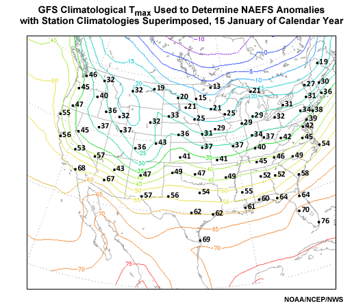
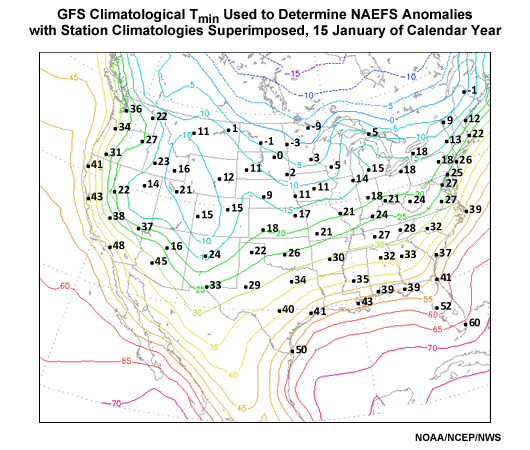
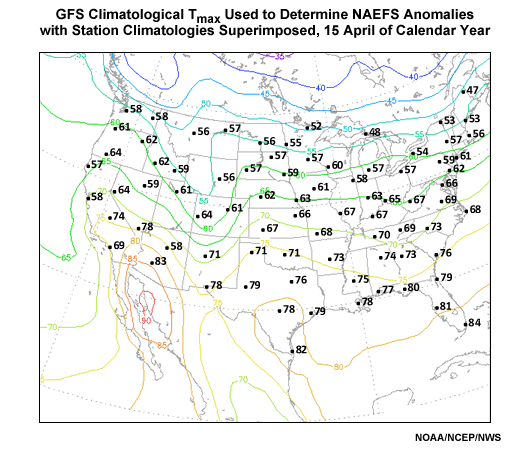
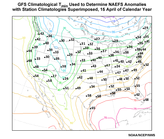
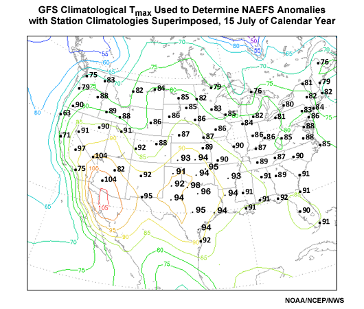
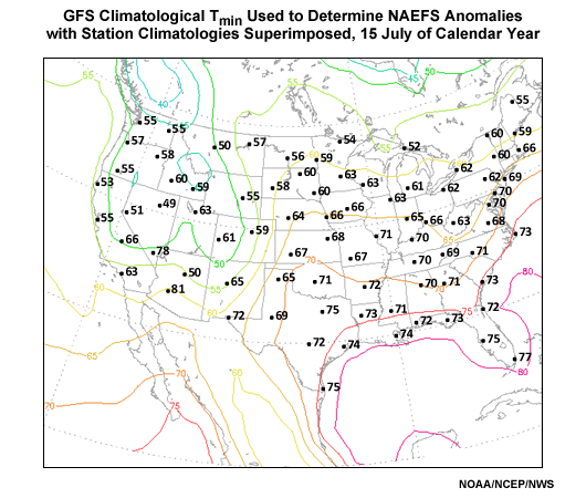
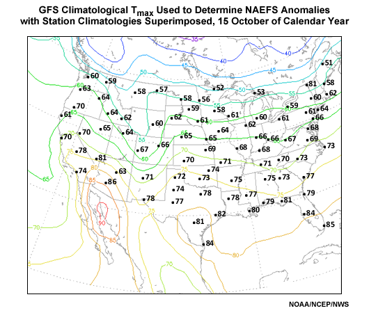
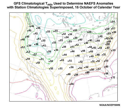
To get a sense for where the analysis bias is significant, graphics showing the contoured analysis climatology with plotted station climatologies for selected locations can be found in Appendix B: GFS versus Station ClimatologiesAppendix B: GFS versus Station Climatologies for January, April, July and October. The problem is largest in the winter season and where the topography is particularly rugged (e.g. the Rocky Mountains and inter-mountain West).
List of Bias-Corrected Fields for GFS/GEFS and CEFS
The bias corrected fields for GFS/GEFS and CEFS ensemble members and for statistical quantities are shown in the table below.
|
Data |
Level |
Variables |
|---|---|---|
|
GFS and individual members from GEFS and CEFS |
Surface |
u/v10m, MSLP, Psfc, T2m, T2m-max, Tmin-2m, mean surface upward longwave flux. 24-hr accumulated precip (GFS, low-res control, first 14 ensemble members only) |
|
1000, 925, 850, 700, 500, 250, 200, 100, 50, 10-hPa |
Z, u, v, T, vertical velocity (850-hPa only) |
|
|
Statistics |
Level |
Variables |
|
Mean, mode, spread, 10th, 50th, 90th percentiles (includes anomalies from GDAS climatology) |
Surface |
u/v10m, MSLP, Psfc, T2m, T2m-max, T2m-min |
|
1000, 925, 850, 700, 500, 250, 200-hPa |
Z, u, v, T |
|
|
Probability of exceedance |
Surface |
24 hour precipitation exceeding
at 6 hourly intervals |
Discussion of NAEFS bias-corrected graphics products can be found in the COMET module Introduction to NAEFS in Section 2, slide 4.
GEFS Bias-Corrected Data for download: ftpprd.ncep.noaa.gov or ftp.ncep.noaa.gov
Bias-corrected data for the GEFS can be found in the following directory:
pub/data/nccf/com/gens/prod/gefs.<yyyymmdd>/<cyc>/pgrb2a_bc/
where
- <yyyymmdd> is the date format (e.g. 20100318 is 18 March 2010)
- <cyc> is the forecast cycle format (e.g. 12 is the forecast cycle beginning at 12 UTC)
Files are in grib2 format with the following name structure for individual ensemble members’ bias-corrected data with the following file naming convention:
ge<pert>.t<cyc>z.pgrb2a_bcf<fhr>
where
- <pert> is the perturbation number
- gfs for the high-resolution operational forecast
- c00 for the low-resolution control
- p01, p02, ..., p20 for the 20 ensemble members, and
- <fhr> is the forecast hour, starting with f00 and going forward at 6-hourly intervals (f06, f12, etc.) to f384
For the statistics, GEFS NDGD downscaled data is available in:
pub/data/nccf/com/gens/prod/gefs.<yyyymmdd>/<cyc>/ndgd_gb2
The file naming convention is:
ge<stat>.t<cyc>z.ndgd_<domain>f<fhr>.grib2
where <stat> is the type of statistic (10pt for 10th percentile, 50pt for median, 90pt for 90th percentile, avg for mean, mode, and spr for spread), <cyc> and<fhr>are as above, and<domain>is the downscaled domain (currently, just the continental US (CONUS)).
GEFS calibrated and raw precipitation probability forecasts for 24-hour accumulated precipitation can be found, respectively, in
pub/data/nccf/com/gens/prod/gefs.<yyyymmdd>/<cyc>/ensstat/enspost.t00z.prcp_24hbc.grib2 and
pub/data/nccf/com/gens/prod/gefs.<yyyymmdd>/<cyc>/ensstat/enspost.t00z.prcp_24h.grib2
NAEFS Bias-Corrected Data for download: ftpprd.ncep.noaa.gov or ftp.ncep.noaa.gov
Statistical NAEFS data for percentiles, mean, mode, and spread can be found in three directories:
pub/data/nccf/com/gens/prod/naefs.<yyyymmdd>/<cyc>/ndgd_gb2, for the downscaled 5-km NDGD statistical products
pub/data/nccf/com/gens/prod/naefs.<yyyymmdd>/<cyc>/pgrb2_an, for the bias-corrected anomalies, and
pub/data/nccf/com/gens/prod/naefs.<yyyymmdd>/<cyc>/pgrb2_bc, for the bias-corrected actual forecast values
Naming conventions for the different statistics files are as for the GEFS above.
Bias Correction as Implemented at NCEP: SREF
The SREF bias correction is performed on each model (i.e. Eta, NAM WRF-NMM, NAM WRF-ARW, and RSM) used in the EFS. A decaying average method is used with a weight of 0.05 (compared to 0.02 for GFS/GEFS/NAEFS) for the current day error and 0.95 (versus 0.98 for GFS/GEFS/NAEFS) for previous day�s decaying average. Errors are calculated through comparison to the respective model control analyses. Unlike the NAEFS, however, no anomalies from analysis climatologies are calculated and output.
Bias-corrected data is written out at 3-hourly intervals as listed below in several different output files.
List of Bias-Corrected Fields
|
SREF Data |
Level |
Variables |
|---|---|---|
|
Individual models/members |
Surface |
u/v10m, MSLP, RH, specific hunidity, T2m |
|
1000, 850, 700, 500, 300, 250 |
|
|
|
SREF Statistics |
Level |
Variables |
|
Probability of exceedance |
Surface |
T2m < 0°C, wind velocity > 25, 34, 50 kts |
|
850 hPa |
T < 0°C |
|
|
Mean and Spread |
Surface |
u/v10m, MSLP, RH, specific humidity, T2m |
|
1000, 850, 700, 500, 300, 250 |
|
When the user review of the bias-corrected data before implementation was completed, the following was noted:
- Bias correction was larger for variables at or close to the model surface
- Bias correction degraded the forecast under the following situations
- During rapid weather regime change
- When errors are weather-regime dependent and the current weather regime is not represented well in the bias correction
- When the bias is small and random errors dominate
SREF Bias-Corrected Data for Download: ftp.ncep.noaa.gov or ftp.ncep.noaa.gov
Files can be found in:
pub/data/nccf/com/sref/prod/sref.<yyyymmdd>/<cyc>/where <yyyymmdd> is the 4-digit year, 2-digit month and 2-digit date, and <cyc> is the forecast cycle (03, 09, 15, or 21). Bias-corrected data files are as follows:
pub/data/nccf/com/sref/prod/sref.<yyyymmdd>/<cyc>/ensprod/sref.t<cyc>z.pgrb<grid>.mean.grib2 where <grid> is the grid number (only 212 currently) for the ensemble mean,
pub/data/nccf/com/sref/prod/sref.<yyyymmdd>/<cyc>/ensprod/sref.t<cyc>z.pgrb<grid>.prob.grib2 for the probability of exceedance products, including temperature below 0C for 850-hPa and 2-m temperature, and
pub/data/nccf/com/sref/prod/sref.<yyyymmdd>/<cyc>/ensprod/sref.t<cyc>z.pgrb<grid>.spread.grib2 for the ensemble spread.
For individual ensemble members' bias-corrected data:
pub/data/nccf/com/sref/prod/sref.<yyyymmdd>/<cyc>/pgrb_biasc/sref_<mdl>.t <cyc>z.pgrb<grid>.<pert>.grib2 where
<mdl> is the model in the ensemble (em = WRF-ARF, nmm = WRF-NMM, eta = Eta, and rsm = regional spectral model).
Appendix B: GFS versus Station Climatologies
The GFS analysis climatology for 2-m temperature is especially prone to model bias, even with being the best analysis available other than the Real-Time Mesoscale Analysis (RTMA). The main problem is representativeness: smoothed topography may result in much different model elevations from actual. Hence discrepancies in 2-m temperature climatology are largest in areas of rugged terrain. Below you will find 1971-2000 station climatologies in degrees F, indicated by numbers, compared to the contoured GFS 2-m temperature analysis climatology, for maximum and minimum temperature.