Table of Contents
- 7.0 Overview
- 7.1 Synoptic Weather Systems
- 7.1.1 Tropical Easterly Waves
- 7.1.1.1 Background and Climatology
- 7.1.1.2 Structure
- 7.1.1.3 Formation of AEWs
- 7.1.1.4 Lifecycle over Africa
- Box 7-1 The Easterly Wave as a Convectively Coupled Wave
- 7.1.1.5 Monitoring and Tracking
- 7.1.1.6 Downstream Transformation (into tropical cyclones)
- 7.1.1.7 Easterly Waves over the Atlantic, Caribbean, and East Pacific
- 7.1.1.8 Intraseasonal Variability
- 7.1.2 Equatorial Inertio-gravity Waves
- 7.1.3 Tropical Upper Tropospheric Troughs and Upper Cold Lows
- 7.1.4 Subtropical Cyclones
- 7.1.5 Monsoon Depressions
- 7.1.6 Arabian Sea Mid-tropospheric Lows
- 7.1.7 Wind Surges
- 7.1.8 Tropical-Extratropical Interactions
- 7.1.1 Tropical Easterly Waves
- 7.2 Mesoscale Weather Systems
- 7.2.1 Mesoscale Definition and Classification
- 7.2.2 Mesoscale Convective Systems
- 7.2.2.1 Thunderstorms and Lightning
- 7.2.2.2 Structure and Lifecycle of Tropical MCSs
- 7.2.2.3 Environments of Tropical MCSs
- 7.2.2.4 MCS Propagation
- 7.2.2.5 MCS Interaction with Large-scale Tropical Circulations
- 7.2.2.6 Global Distribution and Impacts
- 7.2.2.7 Heat and Moisture Transport
- 7.2.2.8 Mesoscale Convective Vortex (MCV)
- 7.2.2.9 Atmospheric Electrical Effects
- 7.2.2.10 Chemical Transport by MCSs
- 7.2.3 Mesoscale and Local Circulations
- 7.2.4 Tropical Severe Weather
- Summary
- Questions for Review
- Appendix 7A
- Brief Biographies
- References
7.0 Overview
In this chapter, we examine the wide-variety of synoptic and mesoscale weather systems that affect the tropics, including, tropical easterly waves, upper tropospheric troughs, subtropical cyclones, and monsoon depressions. Extratropical interactions, such as those caused by Rossby wave trains and the MJO, are examined. This chapter presents a review of thunderstorms and lightning. The structure, formation mechanisms, and hazards of mesoscale convective systems are examined. The distribution of lightning globally and within mesoscale systems is examined. Mesoscale and local circulations, such as sea-breezes, are explored. The final section focuses on severe local storms such as tornadoes and waterspouts.
Print Version
The print version provides a single printable page with all required content.
Multimedia Version
The multimedia version provides structured page navigation.
Quiz and Survey
Take a quiz and email your results to your instructor.
After completing this chapter, please submit a User Survey.
7.0 Overview »
Learning objectives
Synoptic systems
- Describe the basic structure, climatology, and hazards of easterly waves
- Describe the basics of easterly wave formation and cite at least one region where they form
- Describe methods of tracking easterly waves
- Describe basic structure and characteristic weather of tropical upper tropospheric lows
- Describe the basic structure and lifecycle of subtropical cyclones and the theoretical mechanisms for their transition to warm-core tropical cyclones
- Describe the basic structure, formation, characteristic weather, and climatology of monsoon depressions
- Describe the sources, extent, duration, and weather effects of wind surges in the tropics
- Describe inertio-gravity waves, their generation, evolution, and coupling with convection
- Explain the formation of Rossby wave trains in the tropics and their impact on midlatitude weather
- Describe how the subtropical jet, the MJO, and atmospheric rivers combine to affect weather in the midlatitudes
- Describe the influence of midlatitude cyclones, fronts, cold surges, and prefrontal troughs on weather in the tropics
- Describe how tropical synoptic weather is affected by the propagation of Rossby wave energy from higher latitudes
Mesoscale systems
- Define the mesoscale
- Explain at least one mechanism of mesoscale instability
- Describe the ingredients needed for thunderstorms and the ordinary thunderstorm cycle
- Describe the basics of lightning formation and the distribution of lightning in the tropics
- Describe thunderstorm downdrafts and their impacts
- Describe the formation, structure, size, and duration of multi-cellular storms
- Recall the structure and lifecycles of common modes of tropical mesoscale convective systems (MCSs)
- List the weather hazards most likely associated with different MCS modes/types
- Identify key environmental features, including large-scale synoptic patterns, that influence MCS initiation and evolution
- Recognize MCSs in satellite and radar imagery
- Compare and contrast tropical and midlatitude squall lines
- Recall the geographic and seasonal climatology of tropical MCSs
- Describe heating and moisture transport in MCSs and their impact on large-scale circulations
- Describe the role of tropical MCSs in atmospheric chemistry and atmospheric electricity
- Describe the formation of thermal circulations (sea/land breeze and mountain/valley breezes) and their impact on mesoscale weather
- Describe ways in which mesoscale circulations, including thermal circulations, interact with other flows
- Describe the formation of non-supercell tornadoes
- Compare the characteristics of waterspouts, tornadoes, and dust devils
- Describe the formation of supercell tornadoes in the tropics (rare but high impact phenomena)
- Recall global tornado climatology
7.1 Synoptic Weather Systems
There is a diversity of weather systems in the tropics, beyond tropical cyclones. Some, such as monsoon depressions, are critical to regional precipitation and others, e.g., squall lines are sources of severe weather. Several weather systems occur preferentially in certain seasons and large-scale circulation patterns. For example, African easterly waves are prevalent during the West African summer monsoon; cold surges occur with Rossby waves that extend to tropical latitudes during winter; and southern Africa experiences heavy rainfall from tropical moisture brought by tropical-temperate troughs (TTT). Some synoptic weather systems are comprised of mesoscale convective systems, although mesoscale systems occur independent of synoptic weather.
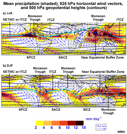
Before examining tropical weather systems in detail, it is helpful to review the major circulations of the tropical atmosphere in which they evolve (Fig. 7.1). These circulations are described in more detail in Section 3.2.2Section 3.2.2 and 9.3.29.3.2.
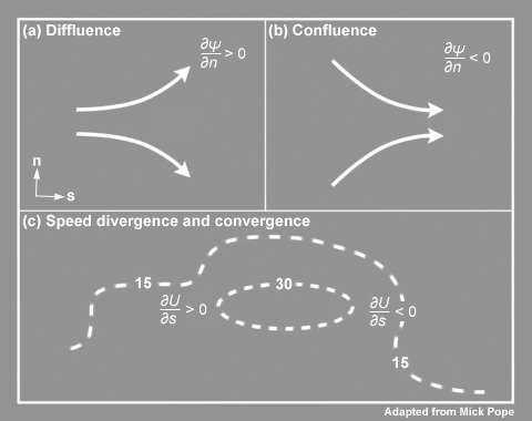
- The ITCZ refers to the zone of confluence between the northeast and southeast trade winds (solid cyan line in Fig. 7.1). Confluence is often associated with horizontal mass convergence but that correlation is dependent on the distribution of the wind speed (Fig. 3.7). The ITCZ is identified as a belt of near-equatorial thunderstorms but these thunderstorms do not form a continuous line; cloud systems within the ITCZ change every day. The ITCZ is referred to by other names, such as the Near Equatorial Trade Wind Convergence (NETWC) in the eastern and central Pacific Ocean and the Near Equator Convergence Zone (NECZ) in the Atlantic.
- The equatorial trough, the belt of surface low pressure due to surplus surface heating and rising motion in the confluence zone, is often but not always co-located with the ITCZ precipitation and clouds. The trough, considered the meteorological equator, migrates farthest from the equator over tropical continents during the summer, while the precipitation maximum remains equatorward of the trough. Regional pressure minima occur within the equatorial trough and are known by regional names, e.g., Saharan Heat Low and Panama Low.
- In monsoon regions, the equatorial trough is called the monsoon trough, which occurs between the trade winds and the westerlies (dashed cyan lines in Fig. 7.1); tropical westerlies are found where the trade winds from the winter hemisphere recurve as they cross the equator. The Near Equatorial Buffer Zone forms where the monsoon winds curve across the equator. Concepts of anticyclonic and cyclonic flow are imprecise in this zone where the Coriolis Effect is negligible.
The meridional movement of the jet streams, tropical cyclones, and subtropical cyclones leads to interactions between tropical and midlatitude air masses. Poleward movement of these weather systems help to maintain low-level convergence zones1 (magenta lines in Fig. 7.1) and maxima in precipitation over the South Pacific Convergence Zone (SPCZ),2 South Atlantic Convergence Zone (SACZ), and intermittent South Indian Ocean Convergence Zone (SICZ).
Synoptic weather systems in the tropics are generally weaker than their midlatitude counterparts (Chapter 3, Section 3.1.4Chapter 3, Section 3.1.4);3,4,5 tropical cyclones are the notable exception. Often the primary circulations of tropical weather systems are prominent in only half of the tropical troposphere with only weak wind perturbations in other layers. For example, fluctuating upper-level cyclones with westerly winds are found above stable trade easterlies, while waves in the low-level easterlies can exist beneath relatively steady upper-level easterlies. The next sections explore the interactions between the lower and upper troposphere and between tropical and extratropical weather systems. The focus is on major weather systems and those that are common to different areas of the tropics, while recognizing that regional variations exist and that similar dynamic and thermodynamic forcing can produce weather systems that may be known regionally by different names.
7.1 Synoptic Weather Systems »
7.1.1 Tropical Easterly Waves
7.1 Synoptic Weather Systems »
7.1.1 Tropical Easterly Waves »
7.1.1.1 Background and Climatology
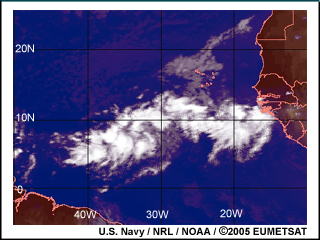
The term tropical easterly wave generally refers to a synoptic disturbance in the tropical easterlies. The most distinctive of these is the African easterly wave (AEW), the dominant synoptic scale weather system affecting tropical Africa, the tropical Atlantic, and East Pacific during summer. These westward moving waves are usually recognized by their associated convection, which is arranged in an inverted V or banded cloud pattern (e.g., Fig. 7.2). The cloud pattern is less defined farther inland but becomes more organized over West Africa. Easterly waves were first recognized in the published literature in the 1930s,6,7 in which rain gauge data analysis showed a periodicity around the three-day timescale. Later, forecasters realized that these same waves moved west to the Atlantic, where some became tropical cyclones8,9 (Fig. 7.2). Some of these waves even survive into the eastern North Pacific basin.10,11
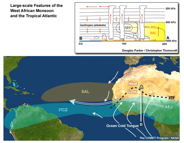
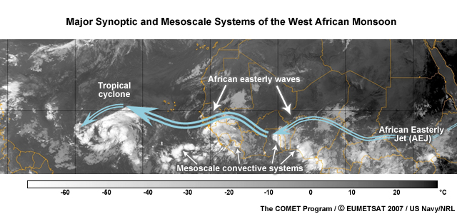
Easterly waves are frequent during the West African monsoon, which has several other major large-scale features, shown schematically in Fig. 7.3. The Sahara Heat Low; cooler, moist low-level monsoon air from the Atlantic Ocean (green shading over land) separated from hot and dry Saharan air by the Inter-tropical Front (ITF; dashed); the Saharan Air Layer (SAL); convection in the Inter-tropical Convergence Zone (ITCZ); and the African Easterly Jet (AEJ; white open arrow). The AEJ results from thermal wind balance and the strong north-south temperature gradient in the low-levels. It is located in the region of strong low-level θ gradients (Fig. 7.3 inset). The jet is easterly because the thermal gradient is reversed with cool air equatorward of warm air to the north. The jet migrates between 8° and 17°N and is strongest between 600 and 700 hPa with speeds of 10-25 m s-1.12
Hazards and Societal Impacts
For the people in West Africa and the Caribbean, the most frequent impacts of AEWs are heavy rainfall and severe weather. AEWs also help to generate and transport of large quantities of mineral dust across North Africa and from there to the Caribbean and Americas,9,13 creating hazards to public health (such as respiratory illnesses) and transportation (reduced visibility). Dust and fungi transported by the waves have been implicated in coral bleaching in the Caribbean.14 AEWs are also important because of their potential for transformation into tropical cyclones in the Atlantic and the East Pacific, although only a fraction of AEWs become tropical cyclones.
Geographic Distribution and Seasonal Cycle
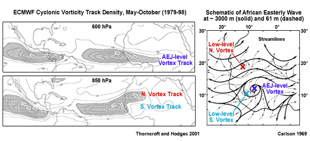
Observations of vorticity maxima show AEW activity along parallel tracks north and south of the AEJ (Fig. 7.4). North of the jet are mainly dry, shallow systems growing along the ITF, with maximum vorticity at or below the 850 hPa level, while south of the jet are moist systems growing mainly at the jet level, with maximum vorticity between 850 and 600 hPa. The two tracks merge over the Atlantic Ocean.
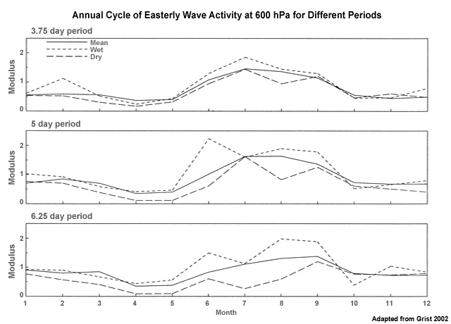
AEWs are most intense and frequent during July, August, and September although they form anytime from May to mid-October (Fig. 7.5). Wave amplitudes tend to be larger in August and September than in June and July. Their seasonal peak and migration is linked to the AEJ seasonal cycle. However, not all waves follow the AEJ cycle; the closest are the 3.75 and 5-day waves. For the southern track waves, peak activity at the 850-hPa level occurs in September.
Compare the AEJ seasonal cycle below with the AEW seasonal cycles above and explain why you think the seasonal cycle of easterly waves does not follow the AEJ cycle.

Feedback:
Wave activity and the variability of deep convection are linked to the vertical shear. The vertical shear is due to both the AEJ and the low-level monsoon flow not just the AEJ. Similar shear is produced by weak (strong) AEJ and enhanced (weaker) low-level monsoon flow.
Interannual Variability
The AEW season is generally longer during wet years and the waves tend to be stronger at 600 hPa. Dry years are marked by reduced wave activity (Fig. 7.5).17 Wet years have been correlated with more intense hurricanes in the north Atlantic.18
7.1 Synoptic Weather Systems »
7.1.1 Tropical Easterly Waves »
7.1.1.2 Structure
The most well-defined AEW, e.g., Fig. 7.6, has the following characteristics:16,19,20,21
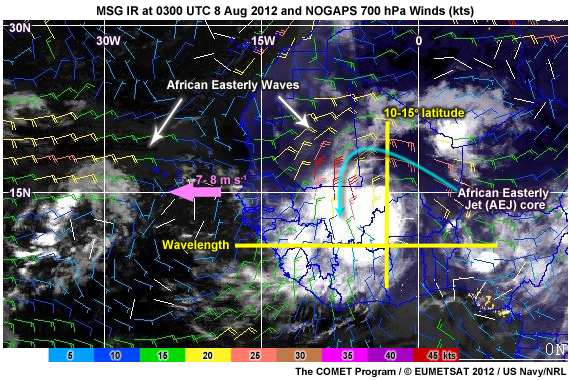
- Wavelength of 2000 to 4000 km
- Period of 3-5 days
- Move westward at speeds of 7–8 m s-1 (about 6–7 degrees longitude per day)
- Latitudinal extent of 10 to 15 degrees
- Maximum amplitude in the low to mid-troposphere
- Exists apart from the ITCZ, although some waves may extend into that zone
An intermittent 69 day wave,22 which has also been observed mostly north of 15°N, has a wavelength of about 5000 km and moves westward at about 6 m s-1.23,24
Composite Horizontal Structure
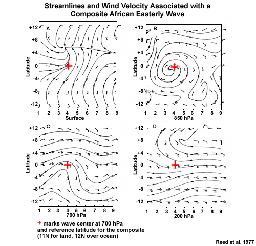
Most AEWs have maximum amplitude in wind speed close to the level of the AEJ, near 700 hPa, and a low-level vorticity maximum near 850 hPa, which is evident in the better-developed cyclonic circulations at those levels for a composite wave (Fig. 7.7). While AEWs occur as waves with maximum amplitude at low-levels and close to the AEJ level,25 both represent a single dynamic mode and propagate simultaneously across Africa. The composite wave has a northeast-southwest oriented axis but individual waves axes can have a southeast-northwest orientation, particularly near the coast. Diffluence is observed around 200 hPa near and ahead of the composite wave.
The composite vorticity field has maximum intensity at 850 and 700 hPa with strong, low- to mid-level cyclonic vorticity ahead and along the wave trough (Fig. 7.8). The stronger southern maximum occurs near the 700-hPa wave center, in the region of moist convection. At 850 hPa the vorticity maximum extends northward and a secondary surface vorticity maximum is to the north. The northern maxima are associated with the ITF, where moist monsoon air meets dry Saharan air.
Ahead (i.e. to the west of) the easterly wave trough is low-level convergence (C in Fig. 7.9), with divergence (D) behind. This pattern is reversed between 700 and 200 hPa: areas of divergence and convergence at 200-hPa occur above low-level convergence and divergence, respectively. Maxima in cloudiness and rainfall are observed ahead of the composite wave trough coincident with the low-level convergence.
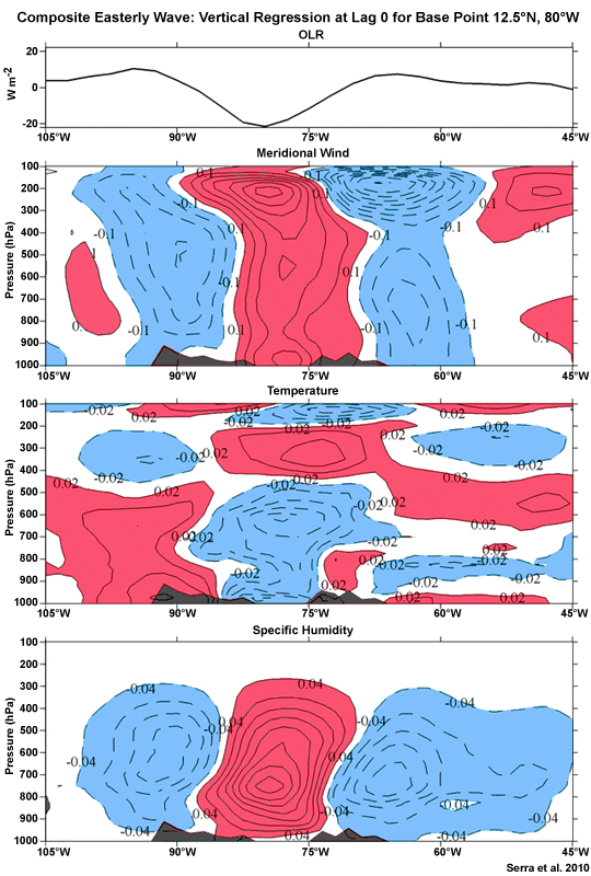
Composite Vertical Structure

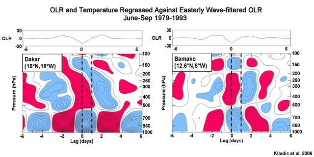
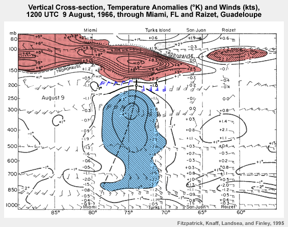
AEWs are generally cold core (blue) up to about 600 hPa with a weak warm core (red) above19,20 as depicted on day 0, the period of AEW trough passage. In this composite wave, the wave structure changes as they move westward from Niamey in the interior to Bamako and then Dakar on the coast. Over the continent, most AEWs have maximum temperature anomalies at the AEJ level; while at the coast, the waves have maximum temperature anomalies between 850 and 950 hPa.
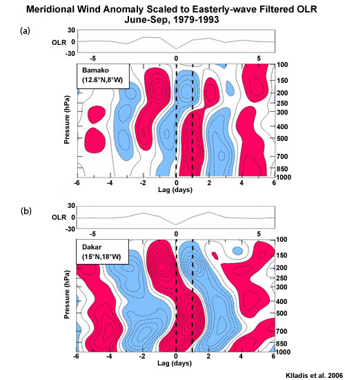
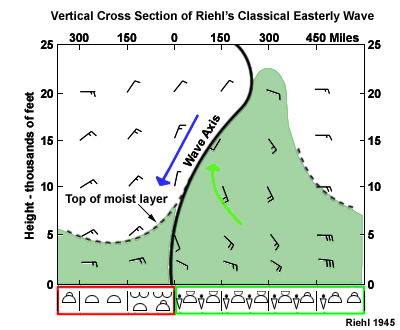
The point at which the meridional winds shift from southerlies (red) to northerlies (blue) is commonly defined as the wave trough at that level (Fig. 7.11). In general, as shown in the composite and in Riehls classical easterly wave model,26 AEWs tilt eastward with height from the surface to mid troposphere AEJ level (~700 hPa) for both Bamako (continental) and Dakar (coastal). However, at Dakar the waves tilt westward above the AEJ.
7.1 Synoptic Weather Systems »
7.1.1 Tropical Easterly Waves »
7.1.1.3 Formation of AEWs
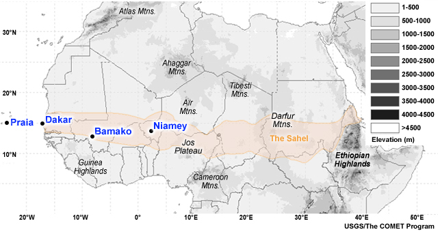
The formation of easterly waves and associated convection is influenced by the topography of tropical North Africa, particularly the Ethiopian Highlands and Darfur Mountains, the easternmost mountains (Fig. 7.12). Most AEWs tend to form somewhere between 15°E and 30°E, downstream of the high terrain. Two main theories have been advanced for the genesis of AEWs:
(i) a linear mixed barotropic-baroclinic instability mechanism and
(ii) finite amplitude forcing upstream of the region of AEW growth.
Another formation mechanism, upstream energy dispersion from an existing wave, was proposed in 2012.27
Mixed barotropic-baroclinic instability
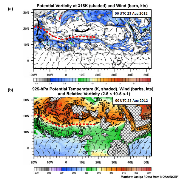
During the warm season over northern tropical Africa, the meridional gradient of the potential vorticity (PV) changes sign near 700 hPa, the AEJ level, i.e., the PV begins decreasing northward (e.g., Fig. 7.13a). Notice the strip of maximum PV south of the AEJ (red dashed line). This sign reversal of the meridional PV gradient satisfies the Charney-Stern criterion for instability of an internal jet.28 Thus, waves are expected to develop from the growth of small random perturbations along an unstable AEJ due to horizontal and vertical wind shear, a mixed barotropic-baroclinic process.29,30,31,32 A climatology of sign reversals of mid-level meridional PV gradients over Africa showed that the sign reversal was generated by concentrated heating from deep convection associated with the active monsoon.33 Coincident with the negative mid-troposphere PV gradient is a strong gradient of potential temperature in the lower-troposphere (Fig.. 7.13b).
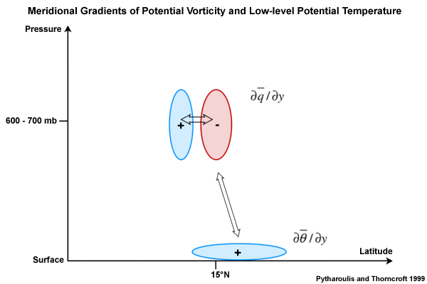
Low-level waves to the north of the AEJ arise due to baroclinic interactions between the negative meridional PV gradients (δq/δy) in the core of the AEJ (~ 700 hPa) and the positive low-level gradient of potential temperature (δθ/δy).25 Arrows in Fig. 7.14 depict the interactions. These dry, shallow low-level waves follow the positive meridional θ gradients over northern Africa, whereas the moist jet-level AEWs follow the meridional PV gradients at the level of the AEJ.
However, the barotropic-baroclinic instability theory has limitations. The AEJ, at 40°-50° longitude, is too short to support more than two waves, so it is not possible to develop AEWs of observed amplitudes solely from this instability mechanism.34,35 Also, simulations show that the AEJ is only marginally unstable, so growth rates are too small to amplify waves at realistic time scales. Still, this dynamic instability strongly influences the evolution and structure of AEWs.
The gradual increase in the intensity of the waves (e.g., Fig. 7.2), as they move towards the coast, is consistent with wave growth by dry baroclinic and barotropic processes. Horizontal shear produced by deep convection near the AEJ contributes to barotropic instability waves can gain energy from barotropic processes if the trough tilts westward with latitude. Vertical wind shear (easterly jet over southwesterly monsoon) plus the moisture, temperature, and pressure gradients contribute to baroclinic instability. Thus, waves can gain energy through baroclinic processes (thermal advection) if the wave trough tilts eastward with height, below the AEJ core (Fig. 7.11).
Upstream forcing
The importance of convection and upstream topography for the initiation of AEWs was suggested by Carlson (1969).9 Recent studies have revisited the role of upstream precursors and support that suggestion.
Thorncroft et al. (2008)36 advanced the idea that AEWs are initiated by local convective forcing near the entrance region of the AEJ. The latent heating creates an initial downstream trough that takes about 5-7 days to reach the West African coast. AEWs are sensitive to the location of the convection; initiation is more efficient when heating creates lower-tropospheric circulations close to the entrance of the AEJ. Thus, the intermittence of observed easterly waves may be explained by the variability of convective activity in this area rather than by considering the jet structure purely. In addition, synoptic-scale simulations suggest37 that the AEJ is of less importance than the heating from ITCZ convection as a cause of easterly wave activity. Mesoscale simulations also suggest that the AEW cannot be sustained for an extended period without active convection.38 For example, precursors to TS Alberto indicate that diabatic heating by convection close to the trough axis enhanced AEW growth rate by producing mesoscale PV anomalies. Bursts of convection preceded the dynamic AEW signal. A significant outbreak of convection over the Darfur Mountains (see map), near the AEJ entrance, favors formation of a train of easterly waves over West Africa within a few days.
Another source of upstream forcing for AEW formation are the upper-level synoptic-scale disturbances that propagate from the east.39 The notion is that the conservation of PV leads to meridional deflection of air parcels when the disturbance moves over the mountains. This mechanism generates cyclonic vorticity and low pressure in the lee of the mountains.40 Although dry PV theory does not allow for lee cyclogenesis when PV is conserved in easterly flow, studies that include moisture10,11 find cyclogenetic regions in the lee of mountains in easterly flow. Additionally, extratropical forcing from midlatitude storms over the North Atlantic can generate AEWs.
Preexisting AEWs
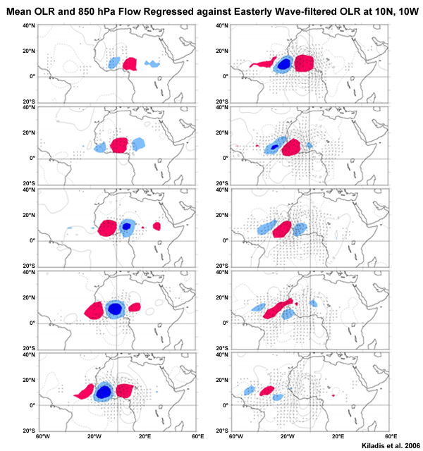
Observations show that new AEWs form preferentially upstream from older waves and that they tend to form in groups. A mechanism has been proposed for AEW formation that is analogous to downstream development of midlatitude baroclinic waves, except that new AEWs form upstream (east) of existing waves. Similar to midlatitude baroclinic waves, the AEW lifecycle can be described by group velocity and dispersion of energy within the wave packet,27 with the energy dispersed upstream (to the east in this case). Hovmöller analysis reveals that eddy kinetic energy is enhanced on the east (upstream) side of AEW wave packets. While individual AEWs are moving to the west, the wave packet meridional wind maximum at 850-hPa moves slowly eastward. While AEWs are moving west, they continue to disperse energy to the east (upstream), which seeds new AEWs.41 This mechanism does not explain the formation of the initial wave but helps explain why AEWs tend to form in groups.
7.1 Synoptic Weather Systems »
7.1.1 Tropical Easterly Waves »
7.1.1.4 Lifecycle over Africa
The initiation and evolution of easterly waves and associated convection is influenced by the topography of tropical North Africa, particularly the mountain ranges (Fig. 7.15).
AEWs are first identified as a weak convective signal in the east (over central Sudan) (Fig. 7.15), eventually attaining their maximum amplitude and intensity near the West African coast. Composite studies identified four regional archetypes in the AEW lifecycle:42
- 20°E recently formed AEWs
- 5°W where AEWs have a tilted baroclinic structure
- 15°W baroclinic tilt is reduced and low-level vorticity is generated south of the jet.
- 30°W loss of baroclinic structure
The change in intensity is illustrated by the amplitude and extent of the anomalies of OLR in Fig. 7.15 (blue represents enhanced convection and red indicates suppression) and the 850-hPa stream function (contours). Waves generally weaken as they move over the eastern Atlantic. However, the eastern Atlantic is also known as the Main Development Region (MDR) Chapter 8, Section 8.6.2.2Chapter 8, Section 8.6.2.2 for tropical cyclogenesis and some AEWs evolve into tropical storms here.
The vertical motion and convection in easterly waves are in phase with a positive mid-tropospheric temperature perturbation, while the surface temperature is at a minimum following the passage of the convection a (Fig. 7.10).
Interaction with convection
Strong correlations are found between 2-6 day-filtered convection and dynamical measures of AEW activity over West Africa.43 Observations show that the Ethiopian Highlands and Darfur Mountains help to initiate AEWs and long-lived convective systems.29,44,45 Convection triggered by high terrain can aid in formation and growth of AEWs through a dynamical feedback between latent heating, vortex stretching, and enhanced potential vorticity in lee (to the west) of these mountain ranges.46,47 Once excited, AEWs propagate westward and grow in response to baroclinic and barotropic instability along the AEJ25,29 (Section 7.1.1.3Section 7.1.1.3).
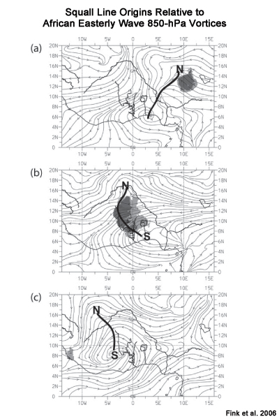
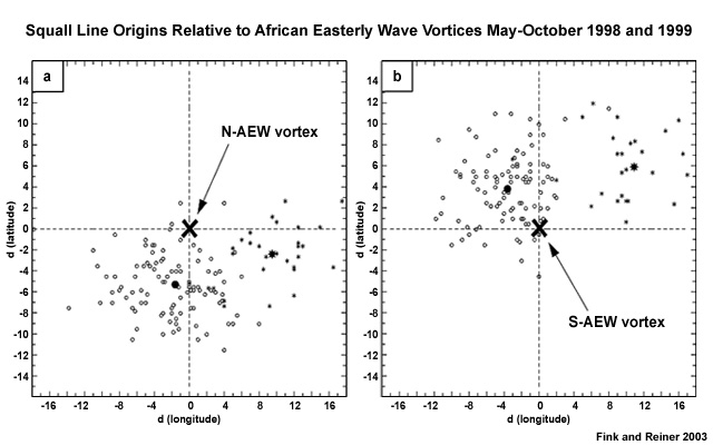
MCSs move with and through the synoptic-scale AEWs, however, MCSs are more influenced by the diurnal cycle over high terrain, convective available potential energy (CAPE, Chapter 5CAPE, Chapter 5), and vertical shear than by AEWs.45,48,49 Deep convective clouds in MCSs commonly occur at or ahead of the AEW trough9,16,24,50,51 but secondary maxima in MCSs occur east of the trough over the northern Sahel45,52,53 (Fig. 7.16). MCSs typically begin east of northern and southern AEW vortices at 850 hPa but at their mature stage, most of the deep convection is west of the southern vortex and east of the northern vortex. MCSs also develop behind the AEW trough and propagate into the region ahead of the AEW trough.
The enhancement of convection at or behind the AEW trough, mainly in the northern Sahel (Fig. 7.17), is primarily influenced by moisture availabilitythe northward transport of moisture from the ocean and equatorial forests.52,55,56,57 For waves along 12.5°N, positive rainfall anomalies are highest in the trough where convection is associated with maximum low-level convergence and cyclonic vorticity, while near 5°N rainfall anomalies are maximized ahead of the trough.56 Peak convective activity occurs east of the trough of intermittent 6-9 day easterly waves.56
Interactions between convection and an easterly wave were observed in detail during the African Monsoon Multidisciplinary Analyses (AMMA) and NASA AMMA (NAMMA) campaigns in AugustSeptember 2006. Oceanic and coastal observations showed that the most intense convection occurred ahead of the wave trough, where high CAPE and low-level convergence were maximized.53 Over the continent, the wave extended the period of precipitation activity for an MCS that was coincident with the 700-mb wave trough. Meanwhile an MCS that originated east of the wave and propagated through the wave trough showed no significant change from its interaction with the wave.
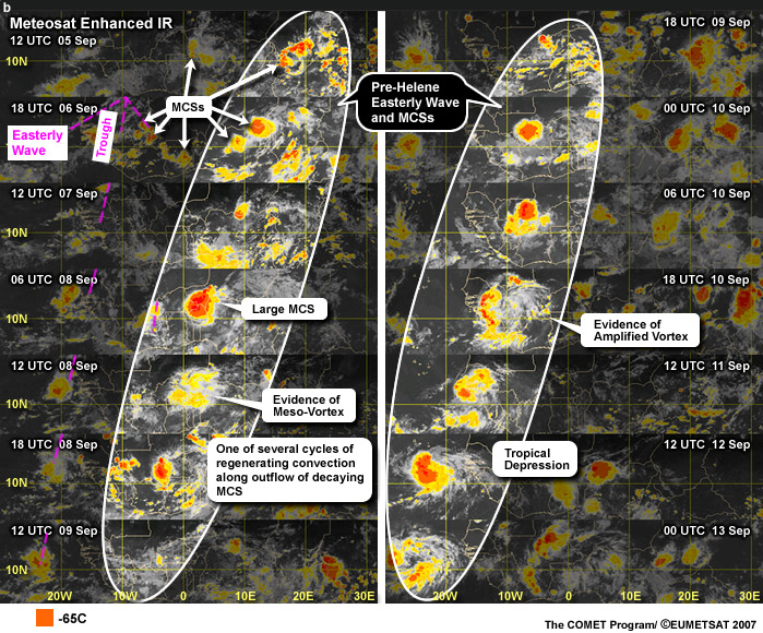
The interaction of the synoptic-scale vorticity associated with AEWs and the mesoscale vorticity associated with MCSs is an area of active research. Some tropical cyclones, such as Alberto (2000), begin as AEW-MCS systems that initiate near the Darfur Mountains and Ethiopian Highlands, and undergo cycles of decay and regeneration while moving westward.46,47 For example, the swirling cloud pattern in the precursors to Hurricane Helene (2006) indicates the presence of a mesoscale convective vortex, a feature that sometimes forms in the stratiform region of MCSs. The pre-Helene vortices appear to amplify over the continent within the AEW structure, a strong vortex emerges from the continent, and tropical cyclogenesis occurs soon after.58 These observations highlight the role of MCSsMCSs as a source of potential vorticity for tropical cyclogenesis.
http://www.amma-international.org/spip.php?rubrique1
NASA AMMA (NAMMA) campaign,
http://airbornescience.nsstc.nasa.gov/namma/
Interaction with surface
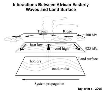
In addition to structural responses of AEWs to the transition between land and ocean, variability in the land surface can also be important. Sharp transitions between bare soil and vegetation and between dry and moist soils are characteristic of the northern Sahel. Soil moisture responds fairly rapidly to variations in precipitation and, in turn, influences convective initiation. The passage of an easterly wave results in wet soils being favored behind the trough (Fig. 7.18) because of the way convection is modulated by the wave. Sensible heat flux patterns are influenced by the zonal contrasts in potential evapotranspiration, which causes perturbation of the 925 hPa isentropes. The perturbed configuration bolsters maximum southerly flow from wet to dry soils, which enhances new convection (Fig. 7.18).
a We say that surface temperature is "in quadrature" with the wave since its extrema lie between the wave troughs and ridges.
7.1 Synoptic Weather Systems »
7.1.1 Tropical Easterly Waves »
Box 7-1 The Easterly Wave as a Convectively Coupled Wave
Like other waves, African easterly waves results from a disturbance or instability that perturbs an initially balanced flow. A wave is created when a restoring force that acts to eliminate the perturbation overshoots its mark. By identifying the restoring force for a given wave type, we can understand the formation and properties of that wave.
Some deep convection in the tropics appears to be organized by dynamics consistent with Matsuno's (1966)60 Shallow Water (SW) theory. These convectively coupled equatorial waves have been identified with prominent spectral peaks in zonal wave number and frequency diagrams developed by Wheeler and Kiladis (1999).61 Those peaks are oriented along the dispersion curves of Matsuno's Shallow Water modes.
Easterly waves are not part of the normal mode solutions to the Matsuno shallow water equations but they were the first convectively coupled tropical wave to be recognized in the published literature.
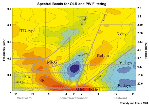
AEWs are off-equatorial, westward propagating Rossby gyres, which are similar in structure to Mixed Rossby-gravity (MRG) waves. They are represented by the Tropical Depression (TD-type) spectral signal, which merges with the MRG signal in the left of the wavenumber-frequency diagram above.
7.1 Synoptic Weather Systems »
7.1.1 Tropical Easterly Waves »
7.1.1.5 Monitoring and Tracking
AEWs do not move smoothly; they accelerate, decelerate, stall, or even retrogress as they respond to diabatic heating from convection at sub-synoptic scales or to surface forcing, or from interaction with midlatitude troughs or tropical upper-tropospheric troughs (TUTTs) over the Atlantic. They move at different speeds over land and over ocean, generally moving slower over the central Atlantic than elsewhere. The movement of easterly waves is also influenced by the interaction of the wave vortex with the Earth's background vorticity gradient, known as the β-effect (Chapter 8, Section 8.7.1Chapter 8, Section 8.7.1). The symbol β represents the north-south gradient of the Coriolis parameter. The rotation of winds around the wave vortex, combined with the northsouth variation in the Coriolis parameter, produces relative vorticity asymmetries, which add a small poleward and westward component to the easterly wave movement over the central Atlantic. Tracking the development and movement of easterly waves requires identification of a reference point, usually the trough axis, using a variety of methods.
Geostationary satellite images
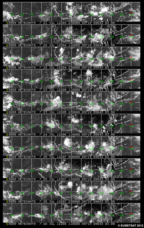
Hovmöller diagrams and animations of satellite images are used to track clouds associated with easterly waves (Fig. 7.19). In this example the area of clouds moves westward from West Africa (0°E) on 21 July to near 30°W by 26 July. However, this method is not consistent for referencing troughs across waves of varied convective signatures and stages of development. Even with a well-defined cloud pattern (banded or circular) unrelated phenomena could be identified as AEWs.
Meridional winds
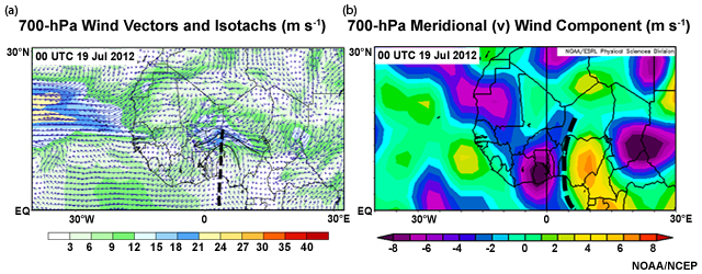
The location where the 700 hPa meridional wind at the level of the AEJ is equal to zero (where the wind shifts from southerlies to northerlies) is commonly used to identify the wave trough associated with the AEW (marked by thick dashed lines in Fig. 7.20). To identify waves to the north of the AEJ, the same method is applied at the 850-hPa level since these waves typically have maximum amplitude at that level.
Relative Vorticity
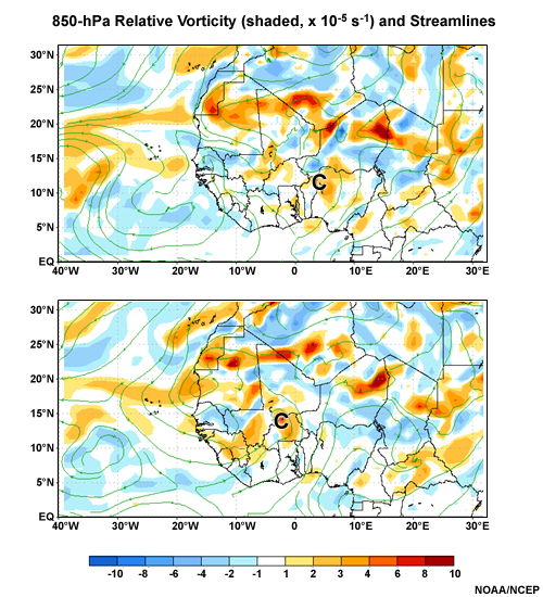
Relative vorticity at 850 and 700 hPa (Fig. 7.21) can also be used to identify AEWs since these waves have relative vorticity maxima at the wave trough at both levels. However, the relative vorticity associated with MCSs is typically stronger than the synoptic-scale AEWs and MCSs move faster on average than the AEWs. These are both complicating factors in the use of relative vorticity maxima for identifying AEWs.
Potential vorticity
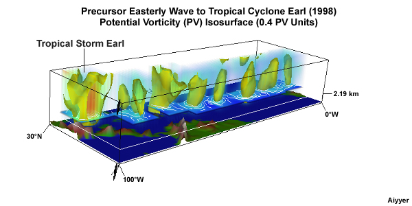
The PV of the low-level vortex north of the AEJ has been identified as part of the synoptic-scale structure of AEWs. For example, about 80% of AEWs in July to September 200463 had a northern vortex that moved with the AEW and were tracked using the maximum PV on the 315K potential temperature surface. PV tracking has the same limitations as relative vorticity; where more than one PV center may be associated with a given trough. Figure 7.22 shows the 3-D PV field associated with TC Earl and its precursor wave.
Time height analysis
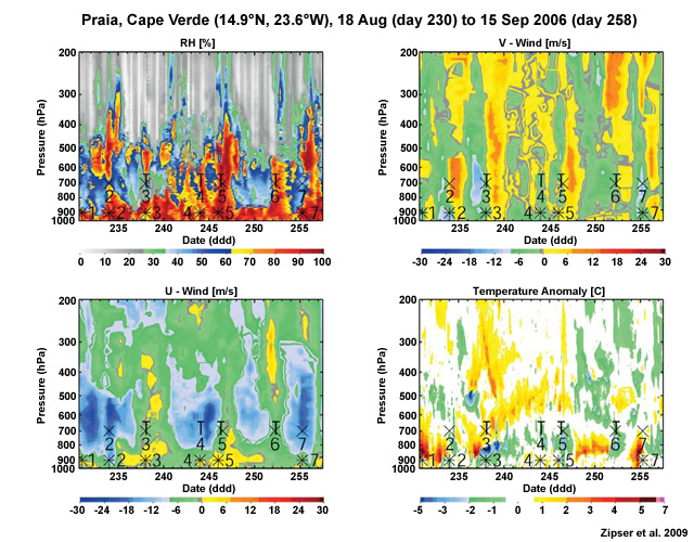
Easterly waves are tracked by analyzing time series of winds, relative humidity, equivalent potential temperature, and temperature anomalies from upper air stations across Africa and the Caribbean. For example, soundings from Praia, Cape Verde (14.9°N, 23.6°W), were used to identify seven AEWs (Fig. 7.23).64 Peaks in relative humidity through deep layers of the troposphere and sharp shifts from northerly to southerly winds occur with the trough passage. Similar to the composite (Fig. 7.9), wave trough passage is generally associated with cool anomalies in the lower troposphere. The wave circulation leads to the zonal winds switching between westerly and easterly direction and the AEJ accelerates behind deep convection in the AEW.
Real-time time-height plots from the National Hurricane Center,
http://www.nhc.noaa.gov/index_station.shtml
Streamfunction
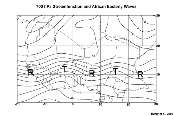
The streamfunction at the AEJ-level (taken to be 700 hPa) is another method for finding the AEW troughs and ridges. The use of streamfunction here is analogous to the use of geopotential height to find troughs and ridges in the midlatitudes. The troughs the streamfunction minima have an inverted V shape (Fig. 7.24).
Advection of the curvature vorticity of the streamfunction
An objective method, developed by Berry et al. (2007),63 defines AEW troughs and ridges as the zero point of the advection of the streamfunction vorticity by the streamfunction wind. Ahead of the trough is positive vorticity advection and behind is negative vorticity advection. The trough is distinguished from the ridge by finding the zero contour of the advection in areas where stream function curvature vorticity exceeds 0.25 × 10⁻⁵ s-1 and flow is easterly. Appendix 7AAppendix 7A lists the equations and the inequalities of diagnostic quantities used to objectively identify axes of AEW troughs and the AEJ.
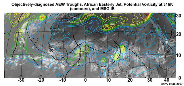
Figure 7.25 shows examples of objectively-identified AEW troughs based on the advection of curvature vorticity of the streamfunction.
University at Albany, Regional maps of objectively identified easterly wave troughs,
http://www.atmos.albany.edu/student/janiga/web/regional_maps.htm
Microwave products from polar and low earth orbiting satellites
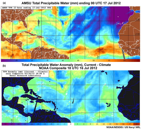
Easterly waves over the ocean can be identified using total precipitable water (TPW) derived from satellite microwave sensors. Fig. 7.26a shows two waves over the tropical Atlantic and one over the Caribbean, near the island of Hispaniola; identified by the inverted V shape in the axis of high TPW. Anomalies of TPW (Fig. 7.26b) sometimes show wave structure more clearly.
Real-time and archived animations of TPW and TPW anomalies,
http://www.ospo.noaa.gov/Products/bTPW/Product_Animation.html
Filtered winds
Winds can be bandpass-filtered for the synoptic-scale to identify AEWs.43 However, this method requires a long time series and approximations of the future state. It is primarily used for research, as it is not reliable for real-time, operational analysis.
7.1 Synoptic Weather Systems »
7.1.1 Tropical Easterly Waves »
7.1.1.6 Downstream Transformation (into tropical cyclones)
Most AEWs weaken as they move westward from West Africa to the relatively cool waters of the eastern and central Atlantic and under the stabilizing influence of large-scale suppression from the subtropical highstabilizing influence of large-scale suppression from the subtropical high. Generally, deep convection decreases and become less organized over the central Atlantic. The eastern Atlantic is less favorable for genesis when the 200-850 hPa wind shear exceeds 15 m s-1.
Transformation into Tropical Cyclones
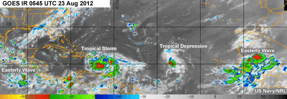
Some AEWs form tropical cyclones (e.g., Fig. 7.27). The most intense hurricanes developed from African easterly waves.18 Sometimes, cyclogenesis occur close to the West African coast and present a threat to life and property because of heavy rainfall, strong winds, and rough seas, e.g., Tropical Storm (TS) Cindy in 1999 caused deaths and damaged infrastructure in Senegal.65 Other waves intensify farther west, some even form tropical cyclones as far away as the East Pacific.10,11 In 1991 each tropical cyclone over the Eastern Pacific was associated with an easterly wave from Africa.66,67
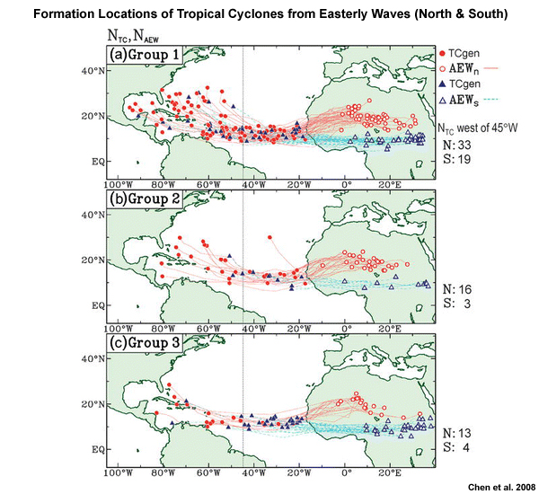
The two dominant AEW tracks, north and south of the AEJ, serve as source regions for tropical cyclones over the Atlantic (Fig. 7.28). The southern track AEWs supply most storms that reach the tropical cyclone MDR of the central and eastern Atlantic and form into tropical cyclones at twice the rate of those in the northern track. Further tropical cyclones forming from southern track AEWs are the source for most of the intense hurricanes (Group 3 in Fig. 7.28). The northern track AEWs travel farther and take longer to transform into tropical cyclones, likely because they are drier and shallower than their south-of-the-jet counterparts.
Developing versus Non-developing AEWs
Several critical differences are found between AEWs that developed or did not develop into tropical cyclones:68
- Developing AEWs have a distinctive cold-core structure about two days before reaching the West African coast.
- Developing AEWs become more warm-cored as they move towards the West African coast.
- In developing AEWs, regions of deep convection are confined to the wave trough at the coast and as they move over the ocean. Non-developers tended to have more intense convection east of the trough.
- Non-developing AEWs have low relative humidity at mid to upper levels north and immediately downstream of the AEWs.
- Non-developing AEWs have weaker amplitudes.
Observations of two developers and a non-developer69 found that, while both types of waves experienced a burst of strong diabatic heating from rapid development of organized convection, the developing waves had a northeastsouthwest-tilted trough axis and wind maximum ahead of the axis and the non-developing wave had a northwestsoutheast-tilted trough axis and wind maximum behind the trough. AEWs often strengthen near the Guinea Highlands because wave vorticity is enhanced by local vorticity generated by terrain-induced convection.70
Differences were also found between AEWs that become tropical cyclones over the Eastern Atlantic and those that evolve into tropical storms farther west, over the Caribbean.71 The wave that developed over the Eastern Atlantic had:
- Enhanced low-level southwesterly flow,
- low-level cyclonic vorticity,
- large-scale low-level wind convergence, and
- vertical motion conducive for development.
The wave that developed over the Caribbean had:
- Strong low- and mid-tropospheric vertical wind shear because of an anomalously strong AEJ,
- lower than normal relative humidity, and
- increased atmospheric stability.
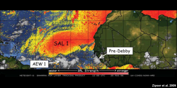
Outbreaks of the Saharan Air Layer (SAL), with its dry air, strong vertical shear, and strong stability, have been associated with inhibited wave development or weakening of tropical cyclones over the eastern Atlantic. In the example shown (Fig. 7.29), the weak, non-developing AEW1 is moving with the region of dry lower-tropospheric air and high dust content (SAL 1) while the Pre-Debby cloud system quickly intensifies in a moister lower troposphere and lower dust content. However, several other factors (listed above) are more critical to the strengthening or weakening of waves than the SAL.
7.1 Synoptic Weather Systems »
7.1.1 Tropical Easterly Waves »
7.1.1.7 Easterly Waves over the Atlantic, Caribbean, and East Pacific
As African easterly waves move away from Africa, different approaches and terms are used to describe, explain, or categorize their transformed structure. Common terms include easterly wave, tropical wave, and inverted V wave. The National Hurricane Center uses the generic term, tropical waves to mean, a trough or area of cyclonic curvature in the trade winds or equatorial westerlies. Riehls classical easterly wave model26 was developed from upper-air observations in the Caribbean while Franks inverted V model73 was developed by observing satellite images of waves in the Atlantic and Caribbean.
According to Riehls classical easterly wave model, waves generally tilt eastward up to the mid-troposphere (Fig. 7.30). The greatest curvature, maximum intensity, is in the mid-troposphere (red streamlines in Fig. 7.30), not at the surface. The white lines depict the trough axis at the surface (west) and between 700 and 600 hPa (east). Winds are generally from the ENE ahead of axis and ESE behind the axis (Fig. 7.30). Wind shifts are weak at the surface, become more pronounced between 850 and 500 hPa and a closed circulation sometimes appears near 700 hPa.
Generally, low-level divergence, subsidence, and fair weather are ahead of the wave over the Caribbean, while convergence, ascending motion, deep layer of moisture, and disturbed weather occur east of the trough (Fig. 7.31). By comparison, convective activity in waves over West Africa is enhanced within or west of the trough and reduced to the east. The exception is in the northern Sahel where convection is also enhanced to the east (similar to the Riehl easterly wave model).

Some waves over the eastern and mid-Atlantic appeared as nested bands of inverted Vs (Fig. 7.32).73 The pattern becomes less distinct as the wave moves westward, in most cases, disappearing near or before reaching the eastern Caribbean. Only part of an inverted "V" may be present in the cloud pattern.
After weakening over the central Atlantic, many easterly waves undergo a temporary blowup of cloudiness over the eastern Caribbean.73 This enhanced cloudiness is most common when the AEW coincides with the southeastern quadrant of a tropical upper-level trough (TUTT) because of rising motion induced by upper-level divergence east of the upper-level trough.
An inverted low-level wave in the easterlies sometimes occurs beneath TUTTs and can be mistaken for easterly waves on satellite images. However, easterly waves are typically steered by the lower-mid tropospheric flow, independent of the TUTT, while the TUTT-induced low-level troughs moves with the TUTT.
The mean profile of easterly waves over the Caribbean and East Pacific derived from a composite study74 (Fig. 7.33) is similar to the Riehl (1945) easterly wave model (Fig. 7.30).26 Both have an eastward tilt up to the mid-troposphere. Cooler temperatures are found in the low to mid-troposphere and warmer temperatures aloft, similar to waves over West Africa. However, in the western Caribbean, the temperature profile is in phase with the southerly phase of the wave, the humidity maximum, and the convection. Over the east Pacific, the maximum wave signature is near 750 hPa.
A near-surface maximum in the meridional wind occurs in the vicinity of the Caribbean Low-level Jet (CLLJ). This implies that interaction between easterly waves and the CLLJ can contribute to tropical cyclogenesis in the Caribbean, either from strengthening waves that originate over Africa or from easterly waves forming in the Caribbean.
7.1 Synoptic Weather Systems »
7.1.1 Tropical Easterly Waves »
7.1.1.8 Intraseasonal Variability
AEW activity is intermittent from May through October, with the tendency for groups of waves to be followed by a period of low activity. Intraseasonal variability in the structure and intensity of AEWs is related to:
- Variability in the regional environment, e.g., shear or convergence associated primarily with the AEJ and also due to the southwest monsoon over Africa
- Variability in how convection couples with different phases of the wave (i.e., troughs, ridges, and in between).
- Variability in how the AEW is initiated
- Interactions with extratropical troughs and with convectively coupled equatorial waves convectively coupled equatorial wave
- Interactions with the Madden-Julian Oscillation (MJO)Madden-Julian Oscillation (MJO)
- Upstream development of other AEWs (leading to eddy kinetic energy dispersion and geopotential flux convergence)
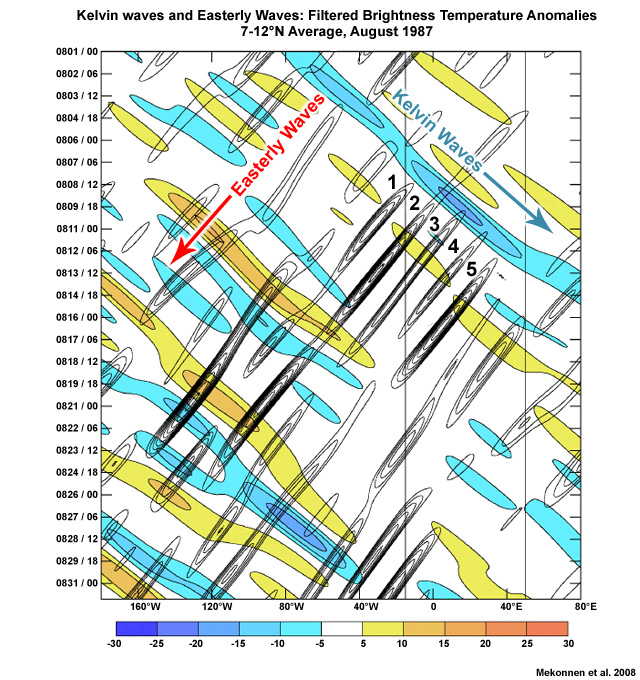
The MJO and Kelvin waves Kelvin waves affect AEW activity by modulating convection over Africa.75,76 For example, five AEWs were triggered or enhanced by a Kelvin wave over Africa during 1987,43 with the fourth of these becoming TS Bret, (Fig. 7.34). Tropical Storm Debby (2006) formed after an AEW interacted with a Kelvin wave over the tropical Atlantic.77 Hovmöller analysis of eddy kinetic energy in AEWs found that, while individual AEWs move to the west, their wave energy maximum moves slowly eastwardtheir wave energy maximum moves slowly eastward. The energy dispersed to the east (upstream) seeds new AEWs, helping to explain why they form in groups.
7.1 Synoptic Weather Systems »
7.1.2 Equatorial Inertio-Gravity Waves
7.1 Synoptic Weather Systems »
7.1.2 Equatorial Inertio-Gravity Waves »
7.1.2.1 Basic Description and Coupling with Convection
The equatorial inertio-gravity (IG) wave is one of a variety of waves that are trapped near the equator due to the reversal of the Coriolis Effect across the equator (Matsuno 1966,60 Chapter 4Chapter 4). It has attributes of a gravity wave propagating in a stably-stratified atmosphere while influenced by both buoyancy and the Coriolis force. IG waves help to organize tropical convection.
 and
and 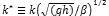 . Eastward propagating waves appear in the right-hand quadrant (relative to the zero basic state employed) and westward propagating waves appear on the left.78
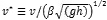
Inertio-gravity waves can propagate eastward (EIG) and westward (WIG) (Fig. 7.35). All of these modes propagate vertically and affect the dynamics of the upper troposphere, as well as the forcing of the quasi-biennial oscillation (QBO, Chapter 4)forcing of the quasi-biennial oscillation (QBO, Chapter 4) of the tropical stratosphere.78 Just as with ocean waves, we describe inertio-gravity waves in terms of their wavelength and period (Chapter 4, Box 4-2)(Chapter 4, Box 4-2), however the axes on the dispersion diagrams (Fig. 7.35) are in terms of variables proportional to the inverse of these quantities: wavenumber (k) and frequency (v). The direction of propagation depends on the sign of the zonal wavenumber, k.
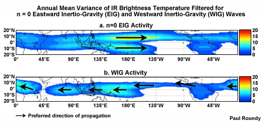
Like other equatorial waves, IG waves are coupled with convection. This convective coupling is measured by outgoing long-wave radiation (OLR), brightness temperature, and precipitation.61 Both coupled EIG and WIG modes have maximum variance over the tropical west Pacific but n=0 WIG variance has another maximum over northern tropical Africa (Fig. 7.36).
EIG waves occur throughout the year but have maximum frequency from May to July and October to December.80 EIG events last for around a week. WIG waves occur throughout the year, but are more frequent during December to February.
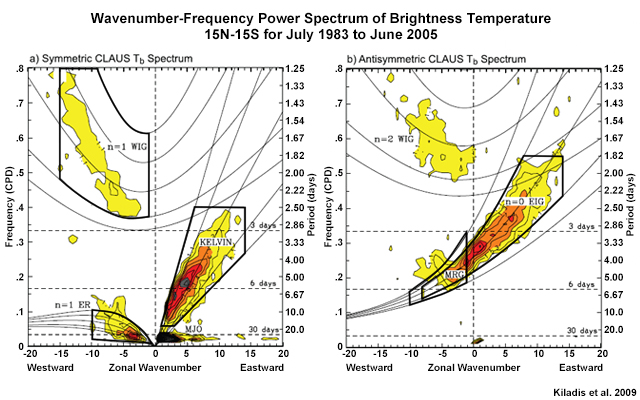
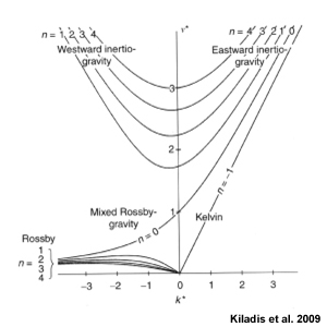
Wavenumber-frequency spectrum analysis of convectively coupled IG waves using OLR61 found peaks (shaded areas in Fig. 7.37) that corresponded quite well to the dispersion relations for dry (theoretical) IG waves found by Matsuno (1966) for equivalent depths equivalent depths of 12 to 50 m. Convectively coupled waves have a shallower equivalent depth than waves without convection, the latter being most commonly observed in the stratosphere.78
Zonal and vertical phase speeds of inertio-gravity waves are fairly fast compared with other equatorial waves. Horizontal speeds range from 10 to > 30 m s-1. The IG spectral maxima show a westward propagating ˜2- to 3-day variance in the symmetric spectrum for the n = 1 WIG wave, and eastward propagating ˜2- to 4-day variance for the n = 0 EIG wave. The anti-symmetric n = 2 WIG is much less studied than the other two wave solutions, although they are detectable in spectra. Note that the spectral peaks of the EIG and mixed Rossby-gravity (MRG) waves are a continuum, even though they are treated as separate disturbances.
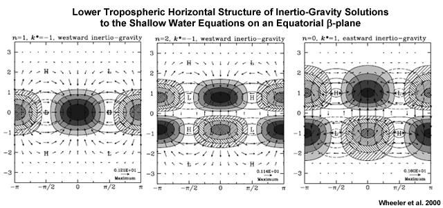
The spatial structure of dry IG waves was first identified by Matsuno (1966); they are the high frequency solutions to the shallow water equations applied on an equatorial β-plane (Appendix 4A1.3)equatorial β-plane (Appendix 4A1.3). Just as the wavenumber, k, defines the number of waves around a latitude circle, the meridional mode number, n, corresponds to the number of nodes each wave has in the meridional direction; a node is a change in sign in the meridional direction of the meridional velocity component of the wave. The curves plotted in Figs 7.35 and 7.37 correspond to different values of n.
The effect of changing either k or n is to change the spatial structure of the wave (Fig. 7.38). The n=1 WIG wave is symmetric about the equator while the n=0 EIG and n=2 WIG waves are anti-symmetric about the equator (Fig. 7.38). The n=1 WIG passage is marked by westward propagation of enhanced equatorial convection then suppressed conditions, similar to Kelvin waves Kelvin waves. Both anti-symmetric waves have off-equatorial convection in one hemisphere and suppression in the opposite hemisphere with low-level flow crossing the equator towards the convective region. The EIG has an extensive area of convergence and predominantly divergent cross equatorial flow from the region of suppression, while the n=2 WIG has a smaller cross equatorial component.
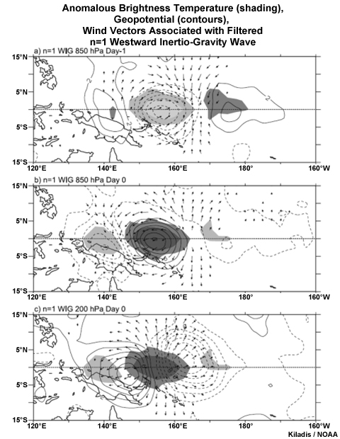
Westward propagating cloud clusters with 1-3 day periods occur over the warm pool of the Pacific and Indian Oceans within the MJO and are termed 2-day waves.81,82 Some 2-day waves have been identified as convectively coupled n=1 WIG82,83,84 disturbances with wavelengths of 2000-4000 km. Composites of n=1 WIG waves show the low-level convergence displaced to the east of the idealized wave solution (Fig. 7.38) but the upper-level matches the idealized structure with maximum divergence co-located with enhanced convection (Fig. 7.39). Simulations of tropical squall lines found that some could be categorized as convectively-coupled inertio-gravity waves with the dispersion properties of shallow-water gravity waves.85 Such features are especially prominent over Africa and the western Pacific.
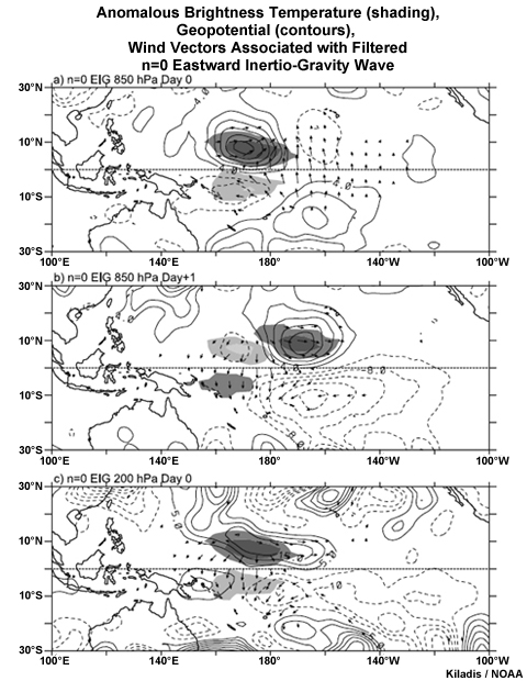
While the n=1 WIG was first identified with deep convective disturbances, the n=0 EIG was better known as a dry stratosphere wave.86 Composites of convectively coupled n=0 EIG circulations do not match well with the relative phasing of convection and motion in the structure of the dry, idealized wave (cf. Fig. 7.38 and 7.40). However, cross-equatorial flow at both low-level and upper-levels is as expected, i.e., 200 hPa winds have a mostly divergent equatorward component, towards the region of enhanced convection.
7.1 Synoptic Weather Systems »
7.1.2 Equatorial Inertio-Gravity Waves »
7.1.2.2 Formation Mechanisms and Theoretical Solutions
Equatorial inertio-gravity waves are usually excited by diabatic heating that induces a large-scale response. A simple model of this large-scale tropical circulation has diabatic heating that peaks in the mid-troposphere; a matching vertical velocity profile, and associated horizontal velocity and pressure perturbation with opposite signs in the lower and upper troposphere (Fig. 7.38). Convection in the WIG waves is phased locked to the diurnal cycle, occurring every other day, which implies that a day is needed for the tropical boundary layer to recover between convective events. It has also been hypothesized that strong shear, particularly in the monsoon regions, may be important to the generation and maintenance of inertio-gravity and other equatorial waves.79
As shown in detail in Chapter 4, Appendix 4A Chapter 4, Appendix 4A, shallow water equations provide mathematical solutions for each of the large-scale equatorial wave types. Both gravity and vorticity (Rossby) waves exist in the shallow water wave equations. Including the Coriolis force gives inertio-gravity wave solutions (rather than pure gravity waves). Potential vorticity (PV) combines measures of rotation and mass distribution, which makes it a useful property for tracking balanced flow structures. Inertio-gravity waves have buoyancy and PV as restoring forces.
To obtain wave solutions, we assume certain conditionsassume certain conditions: the waves are perturbations with respect to some background state, the background state is a fluid at rest with a desired mean depth, and for the Tropics, a constant easterly zonal flow is assumed. At high frequencies, the Rossby wave frequency can be approximated by the equation:
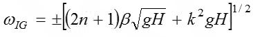 (1)
(1)where ω is the wave frequency, k is the zonal wavenumber, H is the equivalent depth equivalent depth of the atmosphere, β is the derivative of the Coriolis parameter with respect to latitude, g is the acceleration due to gravity, and where n is an integer resulting from the series solution of the wave equation. As discussed above, n is the number of modes in the meridional component of the wind that is associated with the wave (places where the v-component goes to zero).
We can infer the sign of the phase speed (and so the direction of wave propagation) by a simple rule: if the frequency, ω, and wavenumber, k, have the same sign, the wave propagates eastward; if they are of the opposite sign, the wave propagates westward. Thus, the positive root of Equation (1) corresponds to eastward propagating inertio-gravity waves (since ω and k have the same sign) and the negative root corresponds to westward propagating inertia-gravity waves (since ω and k have opposite signs). The signs of ω and k come out of the solutionssolutions to the shallow water equations.
The spatial structure of the wave in each propagation direction can be derived by assigning an appropriate value for n in Equation (1) and solving for the meridional wind component. Substituting this solution back into the shallow water equations will give the wave form for the zonal wind and the height perturbation. For n=0, the positive solution is for the eastward inertio-gravity wave, and the negative solution corresponds to MRG waves. Details of the derivations of equatorial wave motion and structure are provided in Appendix 4CAppendix 4C, with inertia-gravity wave solutions in Appendix 4C.3Appendix 4C.3.
7.1 Synoptic Weather Systems »
7.1.3 Tropical Upper Tropospheric Troughs and Upper Cold Lows
7.1 Synoptic Weather Systems »
7.1.3 Tropical Upper Tropospheric Troughs and Upper Cold Lows »
7.1.3.1 Structure, Weather, and Climatology
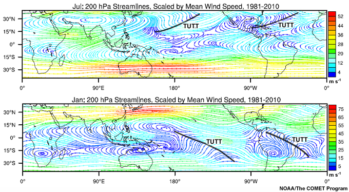
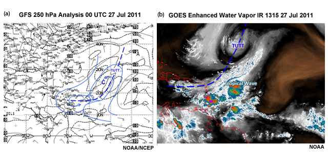
TUTTs are persistent features of the warm season in the Atlantic and Pacific Oceans87 (Fig. 7.41). They can be detected as cyclonic circulations in the westerly winds between 200-300 hPa with the trough axes extending diagonally from the subtropics westward to the equator, e.g., oriented SW-NE over the northern hemisphere.88
TUTTs are cold-cored and exist mostly above 500 hPa (e.g., Fig. 7.42). They spawn upper cold core lows called TUTT cells, which give rise to deep convective clouds and precipitation, which tend to be on the south and east sides of the trough. These cold lows are 2000-3000 km wide with their circulation between 100-400 hPa. They move west and slightly equatorward at 3-5 m s-1 and last for about 1-2 weeks.
TUTTs sometimes induce inverted troughs in the low-level easterlies. These inverted troughs can be mistaken for easterly waves when viewed by satellite. However, TUTT-induced troughs are usually associated with broad areas of high clouds that move with the upper-level flow, while easterly waves move independent of the upper-level flow, being steered by low-mid level flow.
7.1 Synoptic Weather Systems »
7.1.3 Tropical Upper Tropospheric Troughs and Upper Cold Lows »
7.1.3.2 Impact on Tropical Cyclones
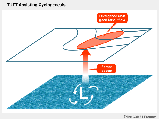
Upper-level divergence east of the TUTT helps to enhance organized convection and can aid in the formation of tropical cyclones from easterly waves (Fig. 7.43). Conversely, TUTTs can hinder tropical disturbances and tropical cyclones from intensifying by introducing large amounts of vertical shear.90
7.1 Synoptic Weather Systems »
7.1.4 Subtropical Cyclones »
7.1.4.1 Structure, Lifecycle, and Impacts
Subtropical cyclones, what are they? They are cyclones that form in the subtropics, about 23°35° latitude.91,92,93,94 Because they have some characteristics of both extratropical and tropical cyclones simultaneously, they present a challenge for classification and forecasting.
Unlike tropical cyclones which typically have an eyewall of deep convection around the surface low pressure center, deep convection in subtropical cyclones is away from the center and is generally asymmetric about the center (e.g., Fig. 7.44).
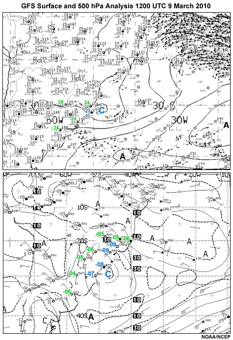
Subtropical cyclones bring clouds, heavy rainfall, strong winds, and severe weather. Subtropical cyclones are cold-core, at least initially, in contrast to warm-core tropical cyclones. Notice the cooler temperatures at the center of the cyclone in Fig. 7.45.
Subtropical cyclones are most common over the subtropical oceans, particularly during the cool season. Those that form in the north Pacific during winter are known as Kona Lows because their southerly winds affect the kona or lee side of the Hawaiian Islands.
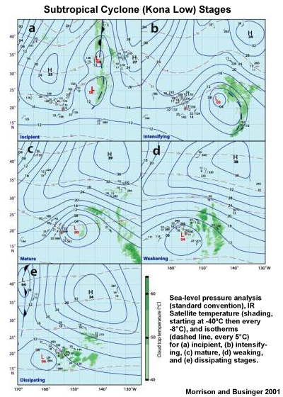
Based on observations of Kona lows, subtropical cyclone lifecycles can be categorized into five stages: (i) incipient, (ii) intensifying, (iii) mature, (iv) weakening, and (v) dissipating. Fig. 7.46 shows the stages for a subtropical cyclone that brought record winds, large hail, high surf, and blizzard to mountainous areas of Hawaii on 24-28 February 1997. Low pressure formed along a quasi-stationary trough. Its early stages had cloud bands near the center but as the low intensified, cloud bands became more pronounced on the east side of the low and farther away from the circulation center. As the cyclone weakened and dissipated, the cloud bands became less organized; thunderstorms were more isolated, and eventually decayed.
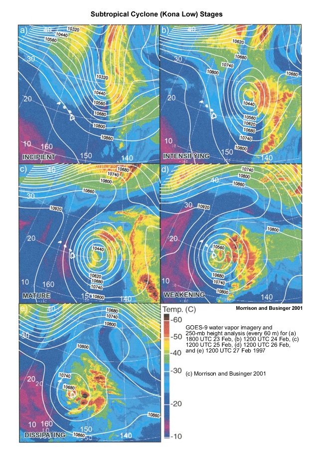
The cyclone at the upper levels is also oriented to the west of the convection as the cyclone intensified (Fig. 7.47). The weakening of the storm is associated with the dry mid-upper tropospheric air intruding into the cyclonic circulation (Fig. 7.47d,e).
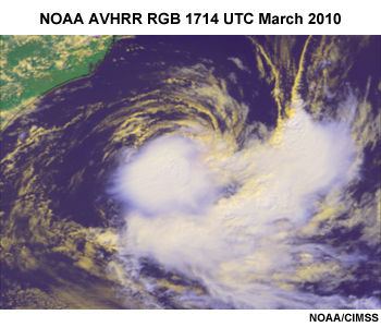
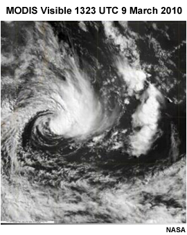
Rather than weakening, some subtropical cyclones transform into tropical cyclones, e.g., the subtropical cyclone off the coast of Brazil (Fig. 7.48) was classified as a short-lived tropical cyclone on 10 March 2010. At that stage, deep convection is found around the surface low (cf., Fig. 7.48 and Fig. 7.44) and the cyclone is more hazardous (stronger winds and more intense convection). The transition of subtropical cyclones to tropical cyclones, termed tropical transition is covered in Chapter 8, Section 8.3.3.2Chapter 8, Section 8.3.3.2.
7.1 Synoptic Weather Systems »
7.1.4 Subtropical Cyclones »
7.1.4.2 Formation and Transformation
Subtropical cyclones form in baroclinic environments but their baroclinicity is fairly shallow and weak compared with cool season midlatitude cyclones. Still, we can approach subtropical cyclone development by examining certain aspects of midlatitude cyclone formation. The development of midlatitude cyclones seems to be dependent on the sign and strength of the barotropic shear added to a midlatitude jet. Breaking of Rossby waves in anticyclonic shear, which occurs when an upper level trough breaks off from the westerlies, results in curved filaments of potential vorticity (PV) in the upper-troposphere.95,96 This upper-tropospheric PV filament can merge into a closed or cut-off low,97,98 which, if it intensifies, may be reflected in an anomaly near the surface.99 A secondary cyclone forms where the upper-level PV filament approaches a surface baroclinic zone. This secondary cyclone forms at lower latitudes than the main cyclone, in the subtropics, hence the name subtropical cyclone. They are distinguished from extratropical cyclones by being isolated from a source of cold air at low-levels. Synoptic analysis often shows a dipole pattern with a cyclone equatorward of an anticyclone.

Two main pathways have been suggested for the secondary cyclone to form, with either extratropical or subtropical processes dominating (Fig. 7.49). In the first case, strong baroclinic forcing, positive vorticity advection and warm air advection, amplifies the upper-level wave and surface front. In the second case, when baroclinic forcing is weak, development is predominantly forced by deep convective heating, with the baroclinic structure serving to organize the heating.100,101 The wave structure enhances the poleward advection and convergence of moist, tropical air. Aided by upper-level divergence east of the upper trough, ensuing deep convection generates an upper-level anticyclonic perturbation.
The role of energetics
The energetics of a subtropical cyclone rely on condensation much more than extratropical cyclones, which rely on baroclinic energy conversions. However, without baroclinicity, the subtropical cyclone would not exist. With intense latent heat release from condensation, the Rossby radius of deformation is reduced,102 which can lead to the formation of a broad variety of disturbances including mesoscale waves or vortices.103,104 Thus, the presence of tropical air with high moisture content combined with baroclinic instability and frontogenesis can generate thermodynamic instability and a substantial convective response, leading to mesoscale cyclogenesis or transition to a tropical cyclone.100,105,106,107
It is important to distinguish between subtropical cyclones and sheared tropical cyclones, which can look similar in satellite imagery. The differences between the two can be subtle. It could be that at higher latitude, a given shear is associated with a greater horizontal temperature gradient through thermal wind balance. Thus the two may be distinct because that crucial characteristic makes the baroclinic conversion of energy nontrivial, while still being less critical than the condensation heating. A substantial amount of research is still needed to distinguish the dynamics of subtropical cyclones from related phenomena.
7.1 Synoptic Weather Systems »
7.1.5 Monsoon Depressions »
7.1.5.1 Structure and Characteristic Weather
The name monsoon depression usually refers to a weak, low-pressure circulation within the monsoon trough that forms in the Bay of Bengal and moves northwestward and westward across the Indian subcontinent during the summer monsoon (June–September).108,109,110 They are persistent rainfall producers, e.g., 400-600 mm of rainfall during 10-15 June 2004 (Fig. 7.50).
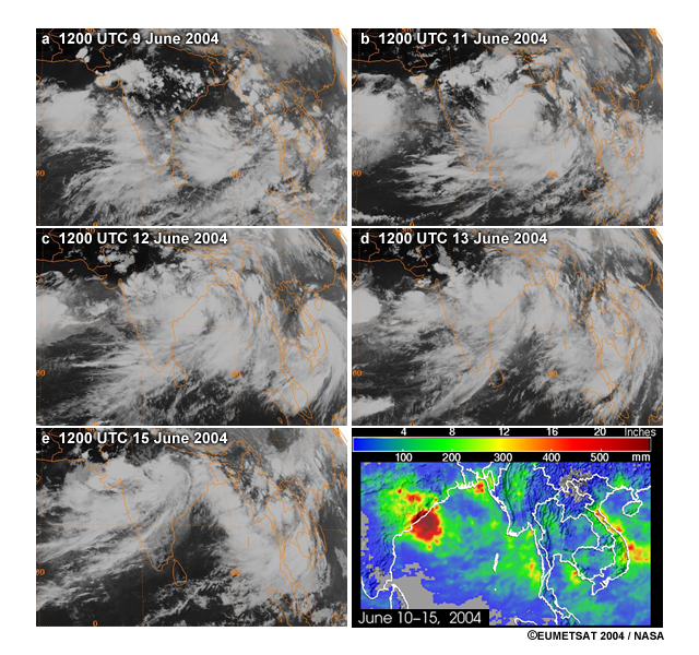
Monsoon depressions,108,112,113,114 like the examples in Fig. 7.50 and Fig. 9.38Fig. 9.38, generally:
- Have a large diameter, on the order of 1000 km (1500-3000 km)
- Have an elongated band of loosely organized deep convection with most rainfall on its southwest or west side
- Lack a distinct cloud center
- Have a small core of light winds, encompassed by stronger gale force winds, but can also have a highly asymmetric wind pattern
- Are strongest below 700 hPa and weaken quickly above that level
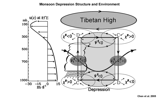
- Extend to about 8 km above the surface (restricted in upward extent by the Tibetan High)
- Produce rainfall rate as high as 100-200 mm in 24 hours
- Move slowly, west or northwestward at 2-6 m s-1 (zonally at 2-5° per day); movement that is counter to strong low-level monsoon flow
The monsoon depression is cold core in the lower troposphere, due to rainfall evaporation and adiabatic ascent, with weak warm core above, which is due to latent heat release. The monsoon trough tilts southward with height, towards the Tropical Easterly Jet. Therefore, monsoon depressions experience strong shear at the upper-levels and do not have the chance to intensify into tropical cyclones.
Monsoon depressions are critical components of the Indian monsoon as they contribute about half of the Indian summer monsoon rain.115,116,117 Because they are large and slow moving, they are persistent rainfall producers, e.g., Fig. 7.50. They bring prolific rain to areas from the Indochinese peninsula to Eastern Pakistan and can remain for days over land, causing floods and related hazards.114 The term monsoon depression has been expanded to include depressions that form within the monsoon trough near Australia and in the western North Pacific region.
7.1 Synoptic Weather Systems »
7.1.5 Monsoon Depressions »
7.1.5.2 Formation and Lifecycle
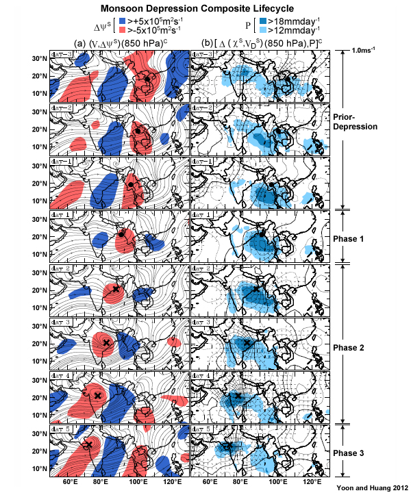
Most monsoon depressions (MD) originate as weak surface low pressure disturbances that come from the west Pacific, South China Sea, and Indochina110,119 and end over the Indian Subcontinent or Arabian Sea. Some residual lows result from tropical cyclones and 12—24-day monsoon lows. The monsoon depression lifecycle can be divided into four phases118,120 (Fig. 7.51).
- Pre-depression (1-2 days prior): Weak precursor low over Indochina with rainfall mainly east of the low.
- Developing (Day 1): MDs tend to develop over the Bay of Bengal when a surface trough is co-located with a wave in the upper-level easterlies. During this development phase, the vortex intensifies due to strong convergence at the low-levels and an increase in water vapor flux over the bay. Most rain now occurs to the southwest of the low.
- Mature (Days 2-4): As the depression moves over land, it produces copious amounts of rainfall as the convergence of water vapor flux increases. With the reduction in insolation, there is less surface evaporation, so moisture increase seems to be due to atmospheric processes (e.g., evaporation from falling rain121,122). Towards the end of this stage, weakening begins.
- Decay (Day 4-5): The depression continues to weaken as it moves farther west, while still producing rain.
Westward propagation
The monsoon depression is remarkable in that it propagates westward against the monsoon flow, which is eastward. Why a lower tropospheric vortex propagates in opposition to the prevailing low-level flow is not fully understood.
The asymmetric structure of the monsoon depression (Fig. 7.52), its heating with heavy rainfall over the west/southwest sector and cooling over the east/north-east sector, seems to play a role in its westward propagation. The center of convergence west of the depression center overlaps the negative streamfunction tendency (Fig. 7.52), which is generated by vortex stretching in the upward branch of the depressions eastwest circulation. This negative streamfunction tendency propagates the depression westward.120 The upward branch of the eastwest circulation is maintained by latent heat release in convection west/southwest of the center, which is then invigorated by convergence of water vapor flux that is coupled with the lower tropospheric divergent circulation. A mechanism that is similar to Conditional Instability of the Second Kind (CISK).123
An alternative hypothesis suggests that propagation is related to the local mid-tropospheric PV maxima within monsoon depressions over South Asia and Australia. Specifically, the westward propagation seems to be due to adiabatic advection of the mid-tropospheric PV maximum.124
7.1 Synoptic Weather Systems »
7.1.5 Monsoon Depressions »
7.1.5.3 Climatology
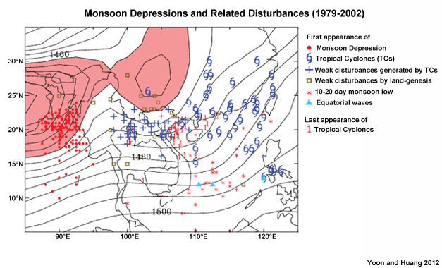
About six monsoon depressions form in the Bay of Bengal each summer monsoon.116 They move at about 5° per day, last for 3-6 days, and produce an average of 25 mm per day with maxima of 100-200 mm per day recorded. Their interannual frequency is highly correlated with the frequency of disturbances over the South China Sea, the vast majority of which move west across Indochina110,119 (Fig.7.53). Their seasonal frequency is related to ENSO, primarily because the precursors of the monsoon depressions form in the tropical Pacific and are thus influenced by the variability of the Pacific sea surface temperature (SST) gradients.
7.1 Synoptic Weather Systems »
7.1.6 Arabian Sea Mid-tropospheric Lows
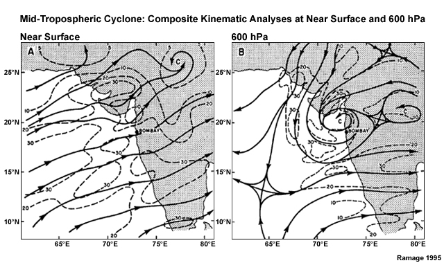
In addition to the monsoon depressions of the Bay of Bengal, the southwest monsoon also spawns mid-tropospheric cyclones along the west coast of India and over the northeast Arabian Sea, and Indochina. These lows form between 700 hPa and 500 hPa in the monsoon trough;125 note the strong cyclonic circulation at 600 hPa compared to the surface flow (Fig. 7.54).
7.1 Synoptic Weather Systems »
7.1.6 Arabian Sea Mid-tropospheric Lows »
7.1.6.1 Structure and Formation
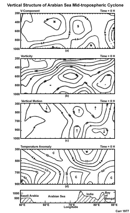
Their maximum intensity is in the mid-troposphere while being hardly detectable near sea level or in the upper troposphere (Fig. 7.55), making them similar to subtropical cyclones in other ocean basins. Vertical motion maxima are related to orographic lift along the Western Ghats and the mid-upper level convergence (Fig. 7.55c). These cyclones are cold core below the mid-troposphere and warm core above (Fig. 7.55d).
How mid-tropospheric cyclones form, intensify, and decay is unresolved as various dynamic and thermodynamic factors combine in their formation. Influences include: cyclonic vorticity exported from the continental heat low, strong moist south-westerly monsoon flow, orography to the east and north, deep layer of convective instability, latent heat release in convection, and upper-level easterlies. Some mid-tropospheric cyclones develop from decaying monsoon depressions.125
7.1 Synoptic Weather Systems »
7.1.6 Arabian Sea Mid-tropospheric Lows »
7.1.6.2 Climatology
These mid-tropospheric cyclones tend to remain quasi-stationary,126 last for about a week, and are the major producers of rainfall along the west coast of India. Some stations average more than 50 mm per day for a week or more. Mid-tropospheric cyclones occur one to four times per season, less frequently and regular as monsoon depressions, and mostly during the first half of the summer monsoon.126
Indian Ocean Surface Streamline pattern,
http://www.usno.navy.mil/NOOC/nmfc-ph/RSS/jtwc/pubref/References/GUIDE/chap2/se103.htm
7.1 Synoptic Weather Systems »
7.1.7 Wind Surges
7.1 Synoptic Weather Systems »
7.1.7 Wind Surges »
7.1.7.1 Trade Wind Surges
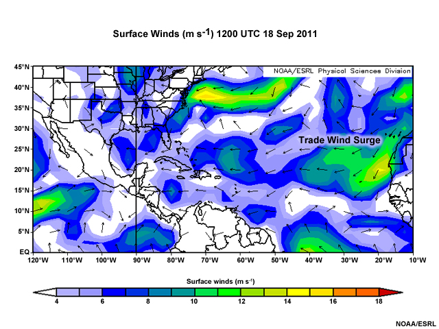
Surges in the trade winds occur when high pressure pulses migrate around the eastern edge of the subtropical high and merge with the trade wind flow (e.g., Fig. 7.56). The confluence of these migratory midlatitude air masses and the trade winds leads to trade-wind surges, synoptic-scale disturbances that move steadily westward. Trade wind surges have periodicity of 5-7 days and trigger convection and rough seas. Surges in the trades have been associated with severe weather and flooding in Venezuela.3
7.1 Synoptic Weather Systems »
7.1.7 Wind Surges »
7.1.7.2 Westerly Wind Bursts
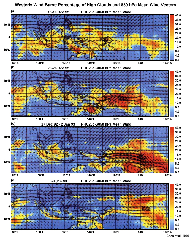
Even over the relatively homogeneous western and central Pacific Ocean, westerly wind bursts (WWB) can produce gale-force winds and increase equatorial convection (Fig. 7.57). These episodes are defined as having westerly winds exceeding 5 m s-1, the wind anomaly is observed at two or more island stations, and persist for at least 3 days. WWBs straddle the equator in a small latitude band (3º-5º) but have a long zonal extent (15°-30° longitude). The typical WWB lasts for 10-20 days and its maximum velocity is most often just south of the equator (e.g., Fig. 7.57). They occur year round but are most common during September to February.
WWB are sometimes caused by cold surges from the winter monsoon (Fig. 7.57b). They are associated with the formation of twin tropical cyclones north and south of the westerly winds,127,128 which occur with Rossby waves trapped along the equator. The formation of a WWB generally leads to increase vorticity on the flanks of the wind maximum; warmer, moist air is advected to the east; the low-level wind shear will change; sea surface becomes mixed and cools the SST by about 0.3°-0.4° C. WWBs also initiate equatorial Kelvin waves,129,130 which help to trigger El NiñoEl Niño as they shift warm surface waters towards the east.
7.1 Synoptic Weather Systems »
7.1.7 Wind Surges »
7.1.7.3 Cold Wind Surges
Examples of wind surges associated with cold extratropical air masses are described in Section 7.1.8.1Section 7.1.8.1, a review of tropical-extratropical interactions.
7.1 Synoptic Weather Systems »
7.1.8 Tropical-Extratropical Interactions
Tropical-extratropical interaction is an important part of the general circulation, the poleward transport of heat and moisture from the tropics, and the global energy and water cycle. Most early studies focused on tropical heating anomalies related to the El Niño-Southern Oscillation (ENSO)131 and their effect on midlatitude weather132,133 (Chapter 4, Section 4.2.1.7Chapter 4, Section 4.2.1.7). Recent focus has been on the MJO and its influence134,135 (Chapter 4, Section 4.1.1.3Chapter 4, Section 4.1.1.3). On the other hand, extratropical forcing affects weather in the tropics,136 particularly during the cool season.
Nearly all instances of tropical-extratropical interaction involve an amplifying Rossby wave that enhances meridional flow or that induces new waves downstream, which then enhance meridional flow.136,137 Extratropical waves bring cold surges and severe weather ahead of advancing cold fronts while tropical air intruding into the midlatitudes produces heavy precipitation, floods, and severe weather.137 In addition, Rossby wave trains are generated downstream of the MJO and equatorial waves. Extratropical intrusion can even lead to cross-equatorial accelerations and initiation of tropical systems, especially in the Asian-Australian monsoon. In this section, we examine synoptic systems in tropical-extratropical interactions and their impact on weather in the tropics and midlatitudes focusing first on impacts in the tropics then on the extratropics.
7.1 Synoptic Weather Systems »
7.1.8 Tropical-Extratropical Interactions »
7.1.8.1 Cyclones, Fronts, and Cold Surges
Cold surges
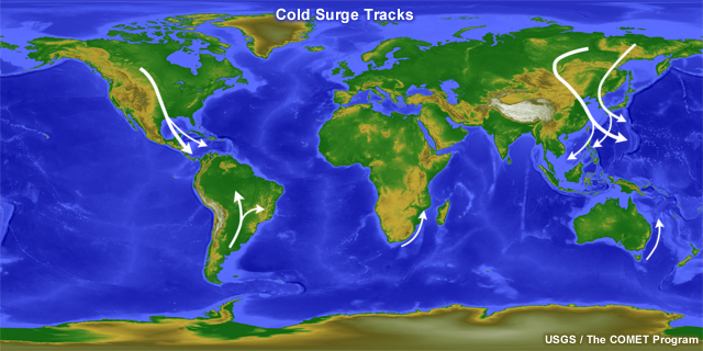
Cold surges into the tropics occur when colder than normal air masses move sufficiently rapidly so that the moderating influence of the underlying warm surface is lessened. They occur commonly where cold air flows equatorward in the lee (east) of major north-south oriented mountain ranges (Fig. 7.58) with the most studied and dramatic cases in Asia138 and the Americas. Other cases that are not as forced by topography can still create hazards, such as North Africa, where strong winds associated with cold fronts can create severe dust storms.
Cold surges in Asia
The Southeast Asian cold surge results from episodic progression of cold, midlatitude air in the lower troposphere moving southward east of the Tibetan Plateau. Cold surges occur mainly during November to March when strong temperature gradients form between the Siberian High and the warm air masses to the south and east. The first signal of the surge is the appearance of northerly winds near 40°N in northern China in association with an upper-level wave that strengthened as it moved from the west towards the coast.139 Then associated surface front and anticyclone moves southward and a cold surge occurs in the tropics within a few days.
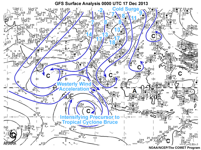
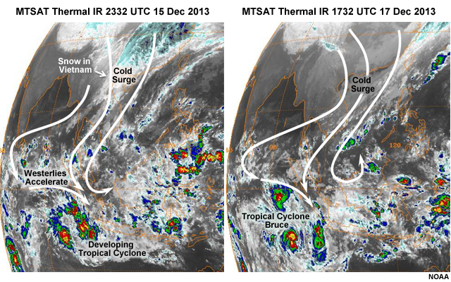
East Asian cold surges usually bring a sharp increase in surface pressure, strong northerly-to-northeasterly winds, an abrupt drop in temperature, and intensification of convective activity over the South China Sea, Borneo, and sometimes the southern hemispheric Maritime Continent140(e.g., Fig. 7.59). The southward penetrating flow interacts with the equatorial trough and the complex topography to trigger organized deep convection and a vortex near Borneo (Fig. 7.59, Chapter 3, Section 3.5.3Section 3.5.3). Some devastating floods in Indochina have been associated with cold surges, which accelerate upslope flow against the Annam Range.141 Extreme precipitation develops when the surface winds are accelerated by the cold surge and a tropical depression141 as happened in November 2013; 700 mm of rain fell in 24 hours and caused more than 40 deaths. The rare occurrence of snow in northern Vietnam occurred with a surge on 16 Dec 2013 (Fig. 7.59). Cold surges in the West Pacific are sometimes associated with westerly wind bursts (Section 7.1.7.2Section 7.1.7.2) and tropical cyclogenesis in the tropical West Pacific.
In East Asia, about 13 cold surges occur every winter season, of which two are strong cases that influence the tropics. The average lifetime of the cold surges is about seven days with strong cases lasting about nine days.142
Cold surges in the Americas
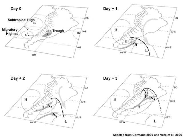
Cold surges in South America typically start with a trough that forms in the lee of the Andes as an upper-level trough and surface front approach the southern tip of the continent from the Pacific Ocean (Fig. 7.60). A migratory surface high behind the front becomes established east of the Andes as the extratropical low moves east. A southeast-northwest oriented cold front separates the high from the warmer air to the north. Strong meridional surface pressure gradients cause southerly winds to accelerate behind the front, advecting cold air northward. The center of the high moves north towards the maximum cold air advection. The extra-tropical air mass advances so rapidly that the cold front moves from near 40°S to north of 10°S in 3 days. Summer time cold surges have a mean speed of about 10 m s-1.
South American cold surges occur most often with surface anticyclone formation (Fig. 7.60) and an upper-level wave east of the Andes.145 The intensifying upper-level ridge helps steer the surface system from the southwest to the northeast. Some rare cases result from surface cyclogenesis along coastal Argentina, which allows polar maritime air to flow equatorward behind the cold front, while upper-level flow is mostly from the west or northwest.145
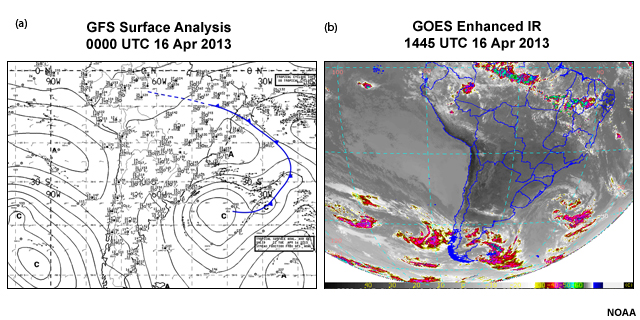
North of 20°S the blocking effect of the Andes is reduced because of its shape, so when the cold front reaches those latitudes the remaining cold air is advected westward. This stage is usually the peak and farthest extent of the extratropical surge into the tropics. Figure 7.61 shows the northern extent of a cold surge that reached 5°N. These types of extratropical incursions occur about every seven days but with varying intensity. Extreme cold surges, known in Brazil as "friagems",146 occur every 2-3 years and cause freezing conditions and damage to agriculture.147,148 Cold air surges in the summer maintain their identities for about 5 days and lead to intense convection, severe weather, and heavy precipitation, triggered by frontal lift and an ample supply of warm, moist air ahead of the cold front.143 South American cold surges can also lead to cloud masses migrating into the Caribbean;149 most likely with a SW-NE oriented subtropical jet over the southern Caribbean, which enhances rising motion.
Cold surges into the Caribbean from the north are less severe than those South American cold surges because of the moderating influence of the Gulf of Mexico and Caribbean Sea. About 15-20% of winter days in the northern Caribbean are affected by fronts, the main synoptic producers of heavy precipitation and thunderstorms during winter.150,151 Fronts in winter typically have a NE-SW orientation152,153,154 and are the leading edge of cold surges that, on rare occasion, can reach the coast of South America.
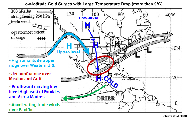
On average 16 cold surges affect Central America annually, with a ±40% change between ENSO extremes.156 About 75% of surges into Central America last 26 days, with those that reach 7°10°N lasting slightly longer than those reaching only 15°20°N.155 How close to the equator the surge reaches depends on where topographic features impede the cold air. Surges are colder when (1) a high amplitude upper-level ridge persists over the western United States, (2) entrance to confluence of the polar and subtropical jet occurs over Mexico and the Gulf of Mexico, and (3) a Canadian lower-tropospheric anticyclone moves equatorward along the Rocky Mountains and the Sierra Madres (Fig. 7.62). Cold surges are also associated with accelerating trade winds over the tropical east Pacific, which is related to ENSO. Sometimes prefrontal troughs develop and cause severe weather and flooding.157
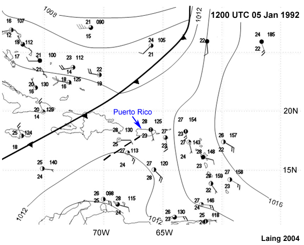
Shear lines
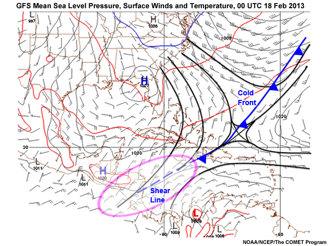
As a cold front moves closer to the equator, the surface temperature and dewpoint gradient across the front becomes very small or non-existent, particularly over tropical oceans. Then only a shear line or shear zone may be present. Shear lines are associated with wind shifts and are usually found by identifying an area of directional wind confluence at the tail end of a front (Fig. 7.63). They may become quasi-stationary and extend for more than 3000 km.
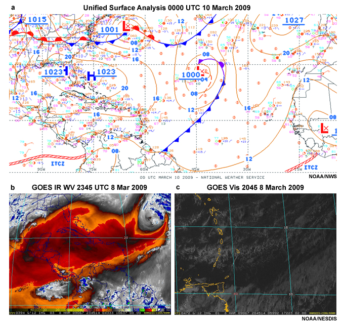
Convergence along shear lines produces cloud lines including thunderstorms. For Central America, passage of shear lines (known as Atemporalado)158 can produce squall lines, gale force winds, and heavy rains. On rare occasions, fronts and shear lines reach into the deep tropics, e.g., in March 2009, when a shear line reached to 5ºN over northeast South America (Fig. 7.64). Such events bring winter rains to the north-facing mountain slopes of Venezuela,152 where they are called invierno de las chicharras.159
Low Latitude Extratropical Cyclogenesis
On extremely rare occasions, the synoptic environment becomes favorable for extratropical cyclones to develop at low latitudes. The ingredients for those events include the combined effects of:
- a low-latitude jet stream; with a
- high amplitude mid-to-upper-level wave, which is conducive to strong meridional temperature gradients and flow;
- an extremely fast jet streak east of the upper-level trough, which promotes strong upper-level divergence in its right entrance region; and
- a surface frontal boundary, which serves as a source of preexisting surface convergence and lift that is aligned with the upper-level divergence.

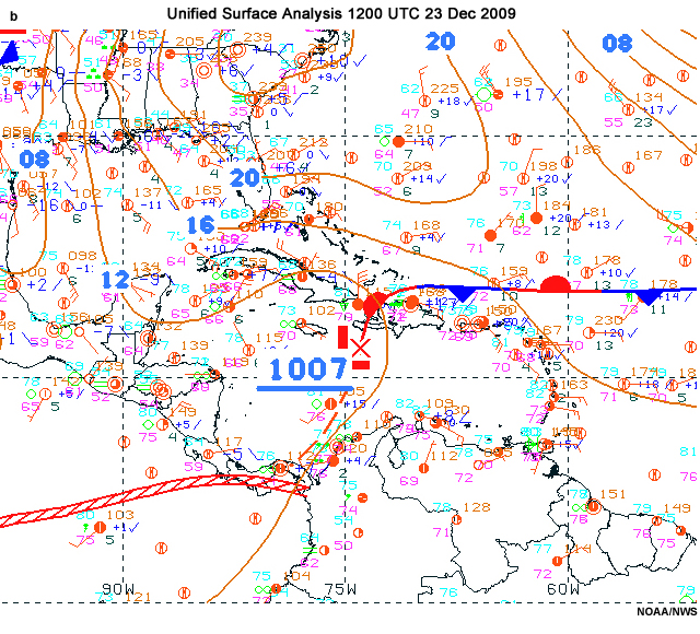
Those conditions occurred in the Caribbean on 22 December 2009 (Fig. 7.65) when upper-level cyclone with a high-amplitude trough extended across the Caribbean into the tropical east Pacific, beyond the equator. The combination of quasi-geostrophic forcing and energy from deep convection along a prefrontal trough induced rising motion and the development of a low pressure center along the front by 1200 UTC 23 December. The intensifying cyclone (Fig. 7.65a) was associated with squall lines and turbulence, which affected flights across the Caribbean, including an American Airlines flight that crash landed in Kingston but did not cause any fatalities. Explore this case in the COMET module, American Airlines Crash Landing in Jamaica, http://www.meted.ucar.edu/radar/tropical_cases/navmenu.php?tab=3&page=1.0.0.
7.1 Synoptic Weather Systems »
7.1.8 Tropical-Extratropical Interactions »
7.1.8.2 Rossby Wave Energy Propagation
Extratropical forcing of tropical convection
Midlatitude upper-level troughs have a significant effect on tropical weather, particularly during the cool season. The intrusion of these extratropical systems can be detected using anomalies of potential vorticity, either on an isentropic surface that represents the subtropical tropopause or averaged over the upper-troposphere/lower stratosphere.
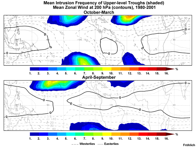
Such extratropical trough intrusions are most frequent over the tropical eastern Pacific, the eastern Atlantic along the West African coast, and east of South America (Fig. 7.66). Favored regions are where upper-level westerlies prevail at low-latitudes, especially during boreal winter and spring.
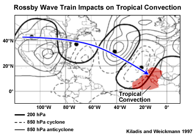
Linear Rossby wave theory helps, but does not fully explain why midlatitude trough incursion occurs in certain regions, seasons, and with some interannual variability. Those regions within the mean upper-level westerlies (known as westerly ducts)161 allow penetration of Rossby wave energy into low latitudes160,161,162 where they can interact with deep tropical convection.163 Figure 7.67 shows an extratropical wave train moving southeastward to the tropical east Atlantic. Mid-to-upper level extratropical wave trains tend to precede mean anomalies in tropical cloudiness over the central Atlantic (Fig. 7.67) and northeast Pacific. Similar interaction occur between wave trains over the SH Indian Ocean and the Australian summer monsoon. Extratropical intrusion can also be tracked at low-levels (thin dashed lines in Fig. 7.67). The waves have a northwest (baroclinic) tilt with height over the extratropics and a more barotropic pattern in the subtropics and tropics. In the NE Pacific, the low level circulations are more complex,160 indicating the need for further study.137
Extratropical forcing of tropical convection occurs with upper-level troughs that tilt east and poleward from the tropics (positive tilt),160 strong cold advection extending deep into the tropics, a front at low-levels, advection of high PV air towards the equator, and a flux of heat and momentum poleward.
Extratropical Rossby Waves and the MJO
MJO impacts on the extratropics are well documented in Chapter 4, Section 4.1.1.3 Chapter 4, Section 4.1.1.3 and elsewhere. MJO convection perturbs the atmosphere and generates eastward and poleward Rossby wave trains,164 exporting tropical moisture and heat to the extratropics165 (e.g, Fig. 4.9). Conversely, studies suggest that the MJO is influenced by the extratropics, e.g., forcing of upward motion by extratropical PV intrusion166,167 and modulation by the MJO-induced waves.168 How and how much of an influence are open questions.
To help answer those questions, the wind field in the tropics can be considered as having three components, using Green's function in free space: 1) a non-divergent component, 2) an irrotational component, and 3) a background or environmental flow. The tropical background flow is understood to result from Rossby wave energy emanating from the extratropics.169 The background flow oscillates with phases of the MJO, closely following variations in the extratropical geopotential heights. The highest coherence is with changes in the geopotential height between 30° and 45° in the Northern and Southern Hemispheres.170
Figure 7.68 is a schematic of the height anomalies associated with an active MJO and extratropical Rossby wave trains. The MJO dynamic signal is a Kelvin wave to the east and equatorial Rossby wave (cyclone pair) in the west. At 850 hPa, ridges over the central Pacific enhance the near-equatorial easterly flow in the Kelvin wave and westerly flow into North America, the latter enhancing coastal precipitation. At 200 hPa, the flow is more complex. An extratropical trough is poleward (upstream) of the MJO equatorial Rossby anticyclonic pair and the downstream Rossby wave train propagates farther downstream than at 850 hPa. The figure illustrates two-way interactions between the tropics and extratropics,168 in which:
- The MJO and other organized tropical convective phenomena induces extratropical waves
- The combined MJO and background circulation can then guide the extratropical Rossby wave train back into the tropics or parallel to the tropics in regions downstream
- The extratropical waves then perturb the equatorial waves,163 thereby influencing the development of convection associated with the MJO, including tropical cyclones
- That convection in turn leads to latent heat release, mass distribution, and disperses energy in Rossby waves to the extratropics, thus creating an interactive feedback process.
7.1 Synoptic Weather Systems »
7.1.8 Tropical-Extratropical Interactions »
7.1.8.3 The Subtropical Jetstream, MJO, and Atmospheric Rivers
Atmospheric Rivers
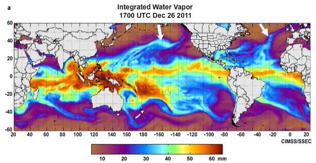
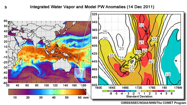
Most meridional transport of tropical moisture occurs via long, narrow channels of high water vapor flux called "Atmospheric Rivers"173 (AR) (Fig. 7.69). At 35°N, about 90% of the total meridional water vapor flux is due to ARs, which cover only about 10% of that hemispheric circumference.173 ARs have strong low level winds and comprise part of the broader warm conveyor belt of extratropical cyclones.137,174,175 The conveyor belt is usually seen as a band of clouds, connecting the tropics and extratropics, that is aligned with the jet stream, and referred to as a "tropical plume",137,176 "tropical moisture exports",177 or "moisture conveyor belts".175,178 The term "Pineapple Express" describes a long-known source of moisture flowing from near Hawaii to the US west coast, before ARs were specifically defined. Note that while tropical plumes are usually associated with ARs, not all plumes are considered ARs.175
Water vapor transport by ARs is usually measured using:
(i) Integrated water vapor (IWV, Fig. 7.69a) and total precipitable water (TPW,179 Fig. 7.69b) derived from microwave satellite retrievals, soundings, reanalysis, or models180 to which a threshold is applied for amount, length and width, e.g., ARs in the northeast Pacific during the cool season are defined by IWV > 20 mm,181 width < 1000 km, and length > 2000 km. Higher IWV thresholds may be better suited to other seasons and regions with higher SSTs. Satellite IWV is measured over the ocean because of difficulties with microwave retrievals over land (Chapter 2, Section 2.5.3Chapter 2, Section 2.5.3).
(ii) Integrated horizontal water vapor transport (IVT) between 1000 hPa and 300 hPa from atmospheric reanalyses or models, e.g., a contiguous region = 2000 km in length with IVT =300 kg m-1 s-1 is used to detect ARs in the Pacific.173,182
The most studied ARs, in the Pacific, are about 400600 kilometers wide and more than 2000 km long.181,183
Atmospheric rivers supply much of the water vapor needed to fill critical water resource needs but also cause disastrous floods along the west coast of the United States, Europe, Northern Africa, and South America, especially where they encounter high terrain.182 At any time, three-to-five major ARs are typically present in each hemisphere (Fig. 7.69a). In a two-year (May 2008 to April 2010) study of global ARs, 259 ARs were observed (122 in the first year and 137 in the second).184 The global maximum is in the northeast Pacific. Regional studies found 15 ARs per year in California182 and about 810 persistent winter ARs in Great Britain.185 The record-breaking 2013-2014 winter floods in Great Britain were due to frequent ARs from the tropical Atlantic.186,187
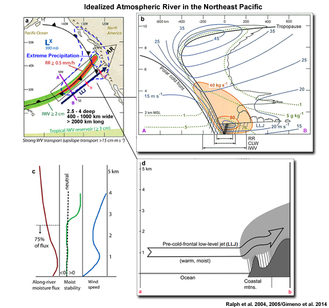
More ARs occur in the winter hemisphere because they occur with extratropical cyclones at subtropical and tropical latitudes, which are more common during winter. A deep layer of concentrated water vapor transport is often found in extratropical cyclone warm sectors and focused in a narrow corridor in the region of the pre-cold-frontal LLJ (Fig. 7.70). Most of the water vapor transport occurs in the lowest 2.5 km, a region of moist-neutral stability (Fig. 7.70c). Large-scale isentropic lift in the warm conveyor belt and convergence along the surface front (Fig. 7.70b) is augmented by orographic lift along western slopes (Fig. 7.70d), particularly in winter when horizontal winds are stronger.
The MJO and Atmospheric Rivers
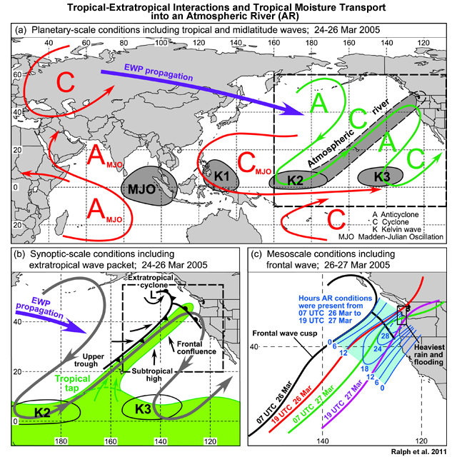
The occurrence of high impact atmospheric rivers on weekly to sub-seasonal scales is influenced by large-scale atmospheric/oceanic phenomena such as the MJO,190,191 equatorial Kelvin waves, and ENSO. For example, flooding along the US West Coast in late March 2005 was the result of interactions between the MJO, Kelvin waves, extratropical cyclones, and a surface front.189 The sequence of events indicates that wave energy is transported eastward from an extratropical Rossby wave train over Asia that coincided with anomalous height perturbations generated in response to tropical convection in the MJO and Kelvin waves (Fig. 7.71). Rossby wave dynamics helps explain the MJOAR relationship (Section 7.1.8.2Section 7.1.8.2). The sequence indicates that wave energy is transported eastward. Additionally, the extratropical cyclone that bears the AR is accompanied by a strong Pacific (subtropical) jet stream, which is consistent with the MJO modulation of the Pacific Jet.192
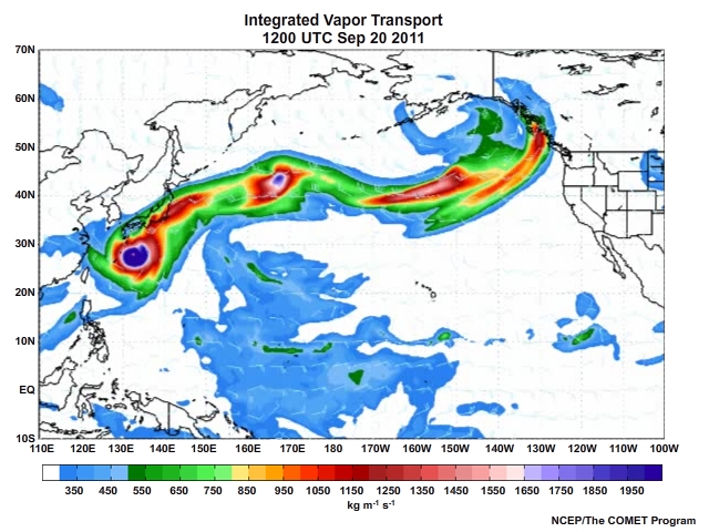
Tropical cyclones in extratropical transition extratropical transition (Chapter 8) are a short-lived source of tropical-extratropical interaction, sometimes comprising part of an atmospheric river (e.g., Fig. 7.72).
http://tropic.ssec.wisc.edu/realtime/mimictpw/global/main.html
NOAA Earth System Research Laboratory:
http://www.esrl.noaa.gov/psd/atmrivers/
TPW and anomaly around the globe,
http://www.ospo.noaa.gov/Products/bTPW/Product_Animation.html
7.1 Synoptic Weather Systems »
7.1.8 Tropical-Extratropical Interactions »
7.1.8.4 Extratropical Interactions with Easterly Waves
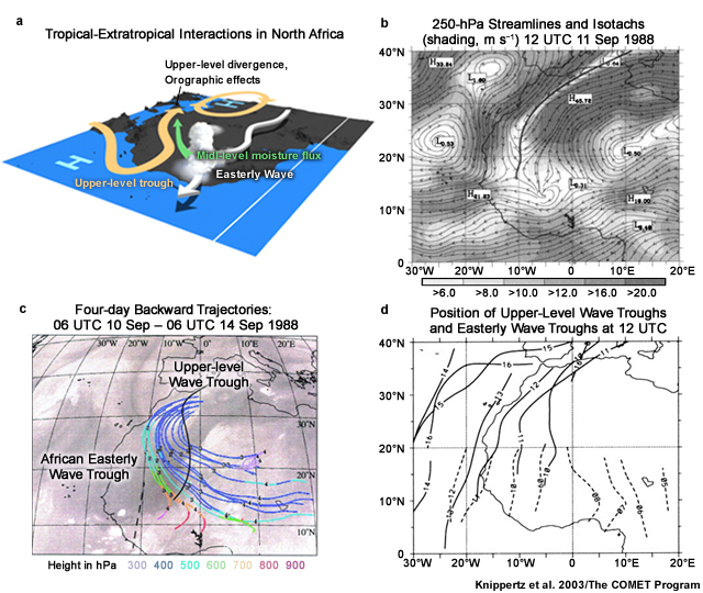
When upper-level midlatitude troughs extend deep into the Tropics, they can interact with AEWs as illustrated for northern Africa. The moisture from the AEW is transported northward to the east of the trough, where moisture converges between 700 and 400 hPa, above the dry Saharan boundary layer (Fig. 7.73). Rising motion is invigorated by upper-level divergence on the eastern side of the trough, resulting in increased moisture and heavy precipitation over Europe and North Africa.

Easterly waves are related to surges into the Gulf of California and the southwestern US. Typically, 1-3 days after the passage of an easterly wave trough over Western Mexico, a surge of low-level moisture is observed at Yuma, Arizona.194 Upward/downward motion associated with the preceding easterly wave trough is indicated by +/- symbols in Fig. 7.74. The low-level moisture from the gulf provides moisture for summertime thunderstorms in Arizona and influence the northern extent of the North American monsoon.
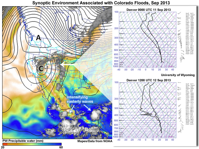
In the western US, the phasing between waves in the midlatitude westerlies and tropical easterly waves can allow moist tropical air to reach high latitudes. Some deadly and devastating flash floods occur when the upper-level trough orientation leads to orographic lift of tropical air by the Rocky Mountains. For example, the deadly and destructive Colorado floods of 11-15 September 2013 resulted when a slow-moving, high amplitude midlatitude cyclone over the southwestern US brought warm, moist tropical air from the tropical east Pacific and the Gulf of Mexico and Caribbean, basins over which easterly waves were intensifying (Fig. 7.75). The "Rex block",195 along the west coast, slowed the movement of the cyclone and its attendant water vapor, clouds, and rain (Fig. 7.75). The upper-level synoptic pattern facilitated the flux of high precipitable water to the midlatitudes. The precipitable water was 36.5 mm and 33 mm on the 11 and 12 September according to the Denver sounding (Fig. 7.75 insets). As the midlatitude cyclone moved east, the easterly waves developed into tropical cyclones and continued supplying tropical air to North America with the worst impacts over Mexico, which had landfalling cyclones on both coasts.
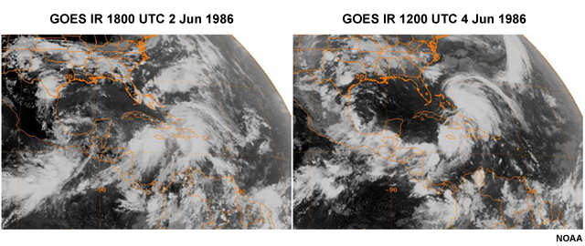
The interaction of easterly waves and extratropical cyclones can lead to flooding in the tropics and tropical cyclone formation. Easterly waves provide lower-level vorticity and the upper-level PV tail of the extratropical cyclone supports synoptically forced ascent. The combination can lead to the transition of a subtropical or extratropical cyclone to a tropical cyclone, e.g., in early June 1986 in the Atlantic (Fig. 7.76). Some of the most devastating floods in the Caribbean occurred early in the warm season, associated with the prolonged combination of extratropical baroclinic forcing, via a quasi-stationary front and upper-level trough, and latent heat release in deep convection from tropical disturbances, supported by an ample supply of warm moist air. Similar synoptic interactions have also led to tropical cyclone formation along the Mei-yu/Baiu front in East Asia.196
7.1 Synoptic Weather Systems »
7.1.8 Tropical-Extratropical Interactions »
7.1.8.5 Tropical Temperate Troughs
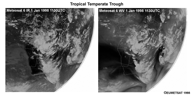
Heavy rainfall during summer in Southern Africa is often associated with tropical-extratropical interactions, evident as elongated cloud bands or "tropical plumes" that stretch from the tropics poleward and eastward to midlatitudes (Fig. 7.77). The synoptic pattern that produces these cloud bands is known regionally as a tropical temperate trough (TTT).197,198 During summer, TTTs are the major synoptic precipitation-producing weather system and are responsible for the majority of heavy rainfall days.199 They export moisture and heat from the tropics to the midlatitudes and may act as a replacement of deep Hadley cell circulations when the ITCZ is weak.
![Maps of 345-K PV(thin contours, PVU), PV advection [thick contours starting at +(-)3 PVU day-1 with positive advection dotted (negative advection solid)] and 345-K diabatic PV tendency (shaded, PVU day-1) on (a) 31 Dec 1997, (b) 1 Jan 1998. Vectors represent 345-K winds >20 m s-1. (c) Moisture transports (vectors, g kg-1 s-1), moisture convergence (shaded, 10-8 g kg-1 s-1), and pressure (contours, hPa) at 309 K for 1 Jan 1998. Regions of moisture export off Africa and into the midlatitudes are noted as warm conveyor belts (WCBs).](media/graphics/ttt_pv_moisture_19980101.jpg)
As observed with tropical-extratropical interactions elsewhere, a low-latitude upper-tropospheric trough is required to facilitate the meridional interaction and formation of the cloud band. In similar manner to the formation of oceanic subtropical cyclones, anticyclonic wave breaking is observed formation of oceanic subtropical cyclones, anticyclonic wave breaking is observed a few days before TTT events.198 The remnant weak PV streamer across the southern subcontinent, in combination with the low PV air aloft and an induced surface low, then initiates poleward moisture transport (Fig. 7.78).
While oceanic tropical plumes have mostly mid- to upper-level cloud in the subtropics, over southern Africa deep convection and heavy rainfall are supported by continental heating and orographic forcing all along the cloud band. In some TTT cases, the baroclinic forcing is weak and deep convective heating becomes the dominant forcing, e.g., MCSs and associated vortex200 migrating around the Angola Low.
7.1 Synoptic Weather Systems »
7.1.8 Tropical-Extratropical Interactions »
7.1.8.6. Tropical Intrusion over South America
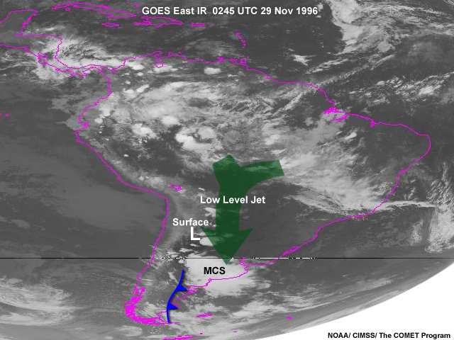
In a similar manner to the TTT in southern Africa, the synoptic evolution of tropical air intrusion in South America can be characterized by the following:
A Rossby wave pattern that aids equator to poleward transport is complemented by northerly prevailing low-level winds and a surface trough over central Argentina. Warm, moist air is channeled southward along the lee of the Andes or from the tropical Atlantic by the South American Low-level Jet (SALLJ) as a cold front moves into southern South America (Fig. 7.79). Low-level convergence increases and northerly flow around the trough intensifies and warm, humid air is advected south to the subtropics and midlatitudes. Extra-tropical MCSs form in the midlatitudes where the cold front meets the convectively unstable tropical air mass; MCSs then move northeastward or eastward ahead of the front. Meridional transport of tropical air and intensification of deep convection is supported by a subtropical jet streak that induces upper-level divergence and rising motion.
![]() Examine the series of satellite images and respond to the questions below. The image color interpretation is provided in the tab entitled, "Image color interpretation".
Examine the series of satellite images and respond to the questions below. The image color interpretation is provided in the tab entitled, "Image color interpretation".
Satellite Animation
Image Color Interpretation
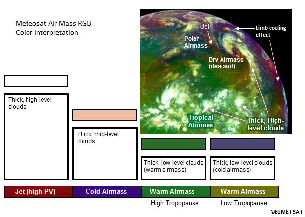
1. What major synoptic features can you identify from the satellite animation? Which of these features is contributing to tropical-extratropical air mass interactions?
(Type your answer in the box, then click Done.)
The ITCZ is marked by a zonal band of deep convective clouds. A tropical moisture plume extends from near equatorial Africa into a cyclone center over the eastern Mediterranean. This plume is contributing to the flow tropical air (green shade) to the midlatitudes. West of the plume is an area of dry, subsiding upper-level air (red-orange shade). Given the cloud and air mass pattern, a surface cold front is likely aligned along the west of the cloud band.
2. What factors are contributing to the formation of the prominent cloud features in the satellite image?
(Type your answer in the box, then click Done.)
The tropical moisture plume is associated with a Rossby wave trough and surface front that extend into the tropics. Upper-level divergence and outflow from deep convection in the ITCZ contribute to the poleward transport of tropical moisture and cloud development in the subtropics and midlatitudes.
3. What is the expected weather associated with this synoptic feature? Examine the meteograms in each tab below and match the meteograms with the locations on the map.

Tab 1
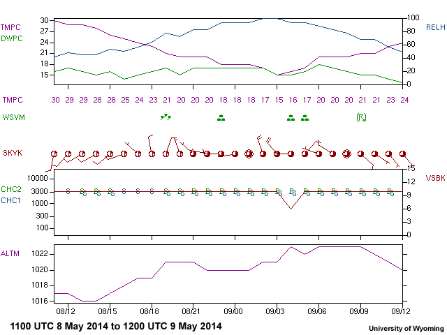
Tab 2
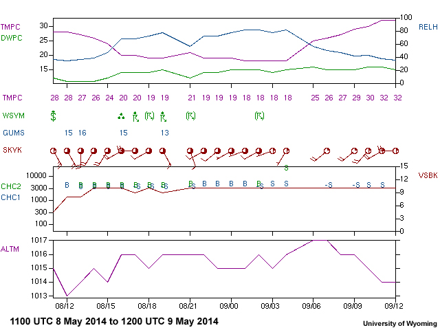
Tab 3
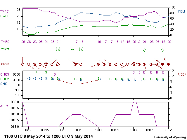
4. How would the weather differ if this synoptic feature were over the ocean?
(Type your answer in the box, then click Done.)
Oceanic tropical plumes have mostly mid-to-upper-level clouds in the subtropics. In this case, deep convection and moderate precipitation are supported by continental heating and orographic forcing in some areas of the cloud band. Notice the differences in the precipitable water anomalies between this plume and an oceanic tropical plume during the same period.
7.2 Mesoscale Weather Systems
7.2 Mesoscale Weather Systems »
7.2.1 Mesoscale Definition and Classification
7.2 Mesoscale Weather Systems »
7.2.1 Mesoscale Definition and Classification »
7.2.1.1 Defining Mesoscale
Mesoscale circulation and systems are generally defined as having horizontal scale on the order of 10 to 1000km, in between synoptic and microscale (Fig. 3.4).201 The spatial and temporal classification of mesoscale202 phenomena is presented in Table 7.1.
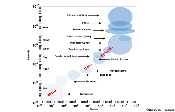
Tropical meteorologists are interested in understanding the mesoscale because most tropical convection is organized on the mesoscale. Mesoscale systems cannot be depicted on ordinary synoptic charts but are of practical importance because most severe weather is associated with mesoscale motions.
| Nomenclature | Spatial Scale | Time Scale | Typical Weather Phenomena |
| Meso-α-scale (alpha) |
200-2000 km | 6h - 36h | Jet streak, small hurricane, weak anticyclone, mesoscale convective complex (MCCs) |
| Meso-β-scale (beta) |
20-200 km | 30min - 6h | Local wind fields, mountain winds, land/sea breeze, large thunderstorms, most mesoscale convective systems |
| Meso-γ-scale (gamma) |
2-20 km | 3 - 30min | Most thunderstorms, large cumulus, extremely large tornadoes |
7.2 Mesoscale Weather Systems »
7.2.1 Mesoscale Definition and Classification »
7.2.1.2 Dynamical Concepts of Mesoscale Circulations
Unlike synoptic-scale systems, where quasi-geostrophic theory and hydrostatic assumptions provide their basic conceptual framework, mesoscale circulations do not have a single dynamical conceptual model. Given the diversity of mesoscale phenomena (Table 7.1Table 7.1), it is not unexpected that dynamical processes will vary. Some mesoscale circulations are hardly influenced by the Earths rotation and vertical motion is non-hydrostatic. For other systems, both ageostrophic advection and rotational influences are important. Such systems can be defined as dynamically mesoscale; their size is close to the Rossby radius of deformation, LR, or they have a Rossby number of order 1. The Rossby radius is defined as
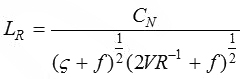 (2)
(2)where ζ is the vertical component of relative vorticity, f is the Coriolis parameter, CΝ is the phase speed of an inertial-gravity wave, and V is the tangential component of the wind at the radius of curvature, R. Figure 3.5 illustrates the scaling of the Rossby radius (Chapter 3, Section 3.1.4Chapter 3, Section 3.1.4).
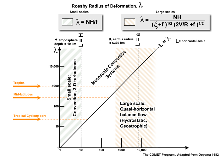
Dynamic stability and the Richardson number
The Richardson Number, Ri, is a measure of the balance between the static stability and horizontal dynamic stability. A fluid can become dynamically unstable because of vertical wind shear, differences in the horizontal velocity between layers of the fluid. Using the Brunt-Väisalä frequency, Ν, as a measure of static stability, Ri can be expressed as
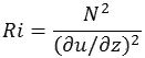 (3)
(3)where u is horizontal velocity and z is the depth or height. Ri can be written as gH/u2 and is calculated to determine if turbulent motion will exist. For small Ri, the shear is enough to overcome the stable stratification. In general:
Laminar flow becomes turbulent when Ri < 0.25
Turbulent flow becomes laminar when Ri > 1.0
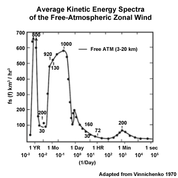
The atmosphere is comprised of a continuity of scales and related energy spectra (Fig. 7.80) but can be approximated by a number of discrete scales. The highest peak in the spectrum corresponds to synoptic spatial scales, while the peak near several minutes corresponds to convection and small-scale turbulence. Atmospheric scales can also be classified according to instabilities of the zonal flow;204 ranging from the baroclinic instability of synoptic midlatitude systems to the small-scale turbulence in the boundary layer, with the Coriolis effect having little influence on the latter.
Mesoscale instabilities can arise through energy transfer from the large scale (baroclinic or barotropic instabilitybaroclinic or barotropic instability) or from the small-scale (cumulus convection or turbulence). Shear-modified Rayleigh instability and Ekman layer instability may aid in the formation of cloud streets and mesoscale cellular convection. Elevated convective instability, typically develops poleward of a baroclinic boundary (e.g., quasi-stationary front) and is associated with a low-level jet oriented normal to the boundary that acts as a conduit for warm, moist air that is lifted over the boundary and initiates elevated convection. Symmetric instability205,206 or slantwise convection is a source of mesoscale instability that is driven by a combination of buoyancy and Coriolis accelerations. Symmetric instability produces mesoscale bands of clouds that form parallel to the thermal wind, e.g., along the Mei-Yu or Baiu front in East Asia Mei-Yu or Baiu front in East Asia.
7.2 Mesoscale Weather Systems »
7.2.2 Mesoscale Convective Systems
A mesoscale convective system (MCS) is an organized, multicellular convective weather system marked by an extensive mid-upper level stratiform cloud shield. Tropical convection is most often organized into mesoscale systems (Fig. 7.81). MCSs encompass a continuous spectrum of phenomena207 including small multicellular storms, tropical squall lines or cloud clusters, bow echoes, mesoscale convective complexes, and even tropical cyclones. They produce heavy rainfall and severe weather, and are vital for the vertical transport of heat, moisture, and momentum. How they develop, grow, and move is determined by variables such as the low-level shear, static stability, and moisture distribution.
MCSs are easily identified from enhanced infrared (IR) satellite (Fig. 7.81). More information about their internal structure is obtained from observations of microwave ice scattering, radar reflectivity, and rain rate (Fig. 7.82). Table 7.2 defines MCSs and intense MCSs based on satellite microwave ice scattering.
| MCS | Minimum area Contour PCT* Minimum enclosed PCT |
2000 km2 250K ≤225K |
| Intense MCS | Minimum area Contour PCT* Minimum enclosed PCT |
2000 km2 200K ≤175K |
*Polarization-corrected temperature (PCT) eliminates emissivity discontinuities between land and ocean and over varying land surfaces. Satellite sensors like the TMI and SSM/I have oblique viewing angles which makes water surfaces highly polarized.
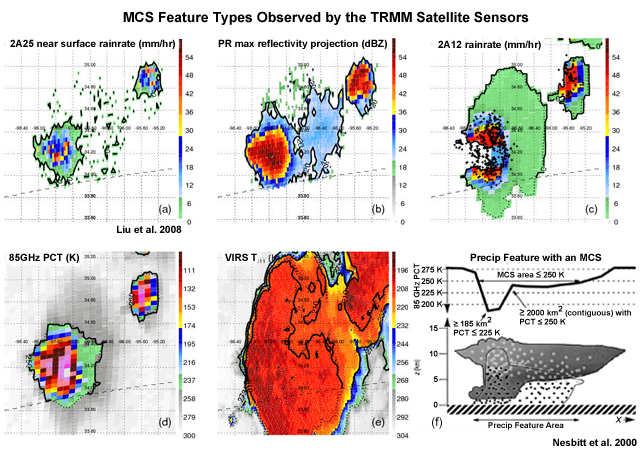
Let us now review the basics of thunderstorms and lightning and then explore different types of MCSs, their structure, lifecycle, large-scale environment, global distribution, and impact on the hydrologic cycle, heat balance, atmospheric chemistry, electricity.
7.2 Mesoscale Weather Systems »
7.2.2 Mesoscale Convective Systems »
7.2.2.1 Thunderstorms and Lightning
Tropical convection exists at an increasing scale from boundary layer cumulus, air mass thunderstorms, supercells, multicellular storms including mesoscale systems, to tropical cyclones. The main ingredient for cumulus convection is moist air that is warmer than its environment, i.e., moist, unstable air (Chapter 5, Section 5.2.2.2Chapter 5, Section 5.2.2.2).

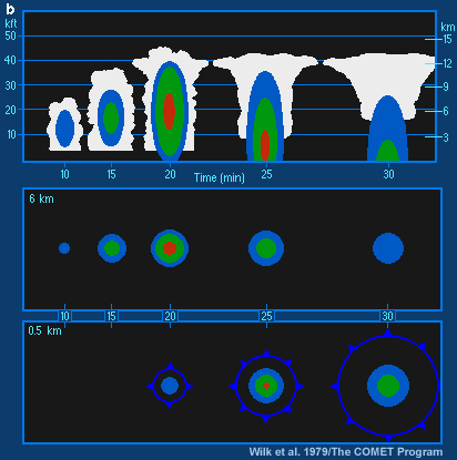
Ordinary thunderstorms
The ordinary or air mass thunderstorm evolution can be described by three stages: cumulus, mature, and dissipating (Fig. 7.83). The cumulus stage begins with a single updraft of air that is warmer than the surrounding environment. Towering cumulus, moisture convergence in the boundary layer, and upward motion are characteristic of the cumulus stage. During the mature stage falling raindrops create a downdraft. The downdraft mixing with drier air in the lower troposphere leads to strong evaporative cooling. The cool air spreads out as a gust front at the surface. Eventually, the downdraft cuts off the supply of rising, moist air in the dissipating stage. Ordinary thunderstorms are typically about 10 km wide, last 20-30 minutes. While generally not severe, they can produce lightning, high winds, and heavy rainfall. Fig. 7.83 illustrates radar echo evolution during the lifecycle of an ordinary thunderstorm.
Multicellular thunderstorms
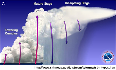
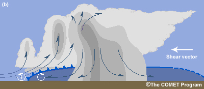
When new cells form along the gust fronts of existing cells, a multicellular storm is born as old cells mature and dissipate and new cells form (Fig.7.84).
The growth of multicellular thunderstorms into mesoscale convective systems depends on the environment in which the initial convection forms. Various parameters are used to evaluate the potential for mesoscale convection to develop. One of the most critical is vertical wind shear, which we will explore further in Section 7.2.2.3. With vertical wind shear, the outflow from a group of short-lived isolated cells can combine into a large gust front (Fig. 7.84). This leads to convergence in the direction of storm motion with new cells forming along and just behind the gust front. The updraft is then separated from the downdraft, which allows multicellular storms to last longer than ordinary thunderstorms.
Lightning
Lightning is one of the primary hazards of thunderstorms. While its formation mechanism is still not well understood, it is known that lightning formation requires the separation of electrical charge in the atmosphere, which occurs in the mixed phase region of tall cumulus clouds where super-cooled water exists with ice crystals. Tropical thunderstorms, which have great vertical extent and whose tops reach the cold, high tropopause, are sources of frequent lightning. Lightning occurs within clouds, between clouds, from clouds to clear air, and from cloud to surface; the latter being the most deadly. The initial path from cloud to ground is usually too fast to be seen, so it is the return stroke from the surface that is identified as lightning.211
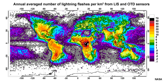
Lightning flash rate is positively correlated with gushes of rain at the surface.214,215,216 However, the amount of rainfall per flash varies by area and rainfall regime. The flash rate of lightning over land is an order of magnitude greater than over the ocean217 (Fig. 7.85). Tropical continents have the highest flash density with the global maximum over the Congo Basin of equatorial Africa. Tropical continents are systematically hotter than oceans, which results in greater instability, larger CAPE, stronger updrafts, deep convection, and thunderstorms.218 Continents are also thought to produce more lightning because of differences in aerosol concentrations.219 It is more polluted over continents, which therefore have more cloud condensation nuclei, which in turn make many small cloud droplets and less rainfall. That in turn allows more liquid water to rise higher into the mixed phase level of clouds where electrification occurs. There is also a marked increase in lightning flash rate with increasing CAPE.220,221,222
https://www.meted.ucar.edu/goes_r/glm/
Lightning video,
http://www.srh.noaa.gov/jetstream/lightning/lightning_max.htm
The Thunderstorm Project,
http://www.srh.noaa.gov/ssd/tstm/html/tstorm.htm
Make thunderstorm, CIMSS,
http://cimss.ssec.wisc.edu/wxfest/MakeTstorm/tstm.html
Thunderstorm downdrafts and their impacts
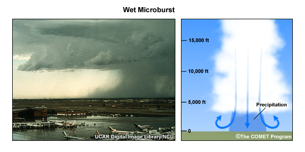
Convective downdrafts are created by precipitation drag, evaporative cooling, and entrainment of dry air. Extremely strong downdrafts can lead to hazards such as microbursts (Fig. 7.86). Microbursts have potential catastrophic consequences for aviation as aircraft experiences sudden loss of air speed and associated loss of lift on encounter with a microburst. The appearance of marked warm areas in cold thunderstorm clouds on enhanced IR satellite images could indicate a strong microburst. The warming occurs as cold air in the upper parts of strong thunderstorms rapidly descends once the updraft collapses; a precursor to strong microbursts.
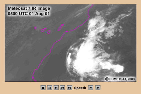
When dry, convective downbursts encounter surface dust, they produce haboobs (an Arabic word for dust storm) (Fig. 7.87). A haboob reduces visibility as dust and sand are lofted upwards by the thunderstorm gust front. Notice the arc of dust (light grey) spreading out from deep convection (bright white) over the Sahara in West Africa (Fig. 7.87).
Explore tropical wet and dry microbursts and their environments in Chapter 9, Focus Section 1Chapter 9, Focus Section 1.
7.2 Mesoscale Weather Systems »
7.2.2 Mesoscale Convective Systems »
7.2.2.2 Structure and Lifecycle of Tropical MCSs
General characteristics
MCSs generally start as cumulonimbus along a convergence boundary in the lower-troposphere, then they merge and organize into a single cloud system with large contiguous rain areas. MCSs contain complex updraft and downdraft structures that reflect the convective and stratiform precipitation areas. The stratiform anvil area results from convective updrafts spreading out in the upper-troposphere and from mescale ascent. As the system starts decaying, the convective cells taper off and the stratiform rain area dominates.
The organization or mode of an MCS is described by variations in the convective and stratiform precipitation structure (along a line or amorphous, leading, parallel, or trailing stratiform). Sometimes different modes occur as stages of an MCS lifecycle.
The structure and lifecycle of MCSs depends largely on the balance between the horizontal vorticity of the cold pool generated by convection and horizontal vorticity associated with the low to mid-tropospheric shear. For long-lasting MCSs, the stronger the Coriolis force, the more asymmetric will be their structure; a major factor in the subtropics and midlatitudes where larger rain areas form on their poleward side.
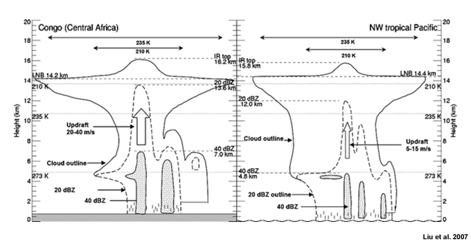
Continental MCSs are more intense than oceanic systems. In general updraft velocities over continents are 2-3 times more rapid than over ocean, leading to taller clouds and deeper mixed phase cloud layer over land. For instance, note the contrast in structure between MCSs over the Congo and those over the northwest tropical Pacific Ocean (Fig 7.88).
Tropical Squall Line MCS
The term squall line generally describes rapidly-moving thunderstorms organized along a line. Tropical squall lines MCSs or squall clusters are usually identified by a line of vigorous convective cells extending for 100-1000 km along its major axis (e.g., Fig. 7.81). In the monsoon regions, squall line MCSs move both eastward and westward in response to the environmental shearenvironmental shear.
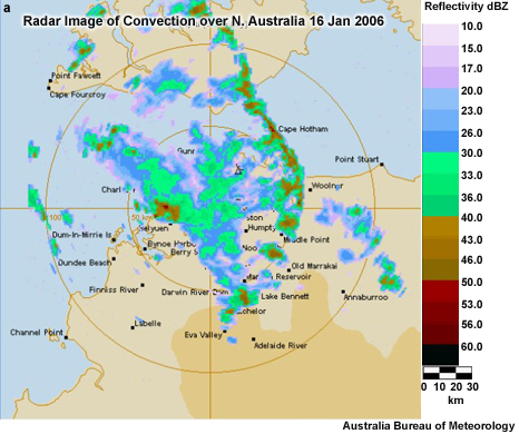
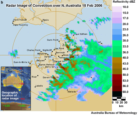
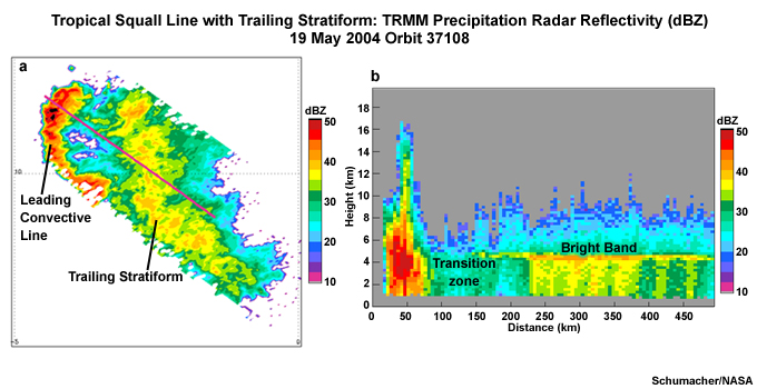
The most commonly-observed squall line structure, in both the tropics and midlatitudes, is the leading convective line with trailing stratiform region (Fig. 7.89). The large cloud shield seen on satellite images, and enhanced growth of precipitation particles, results from sloping deep-layer ascent in the stratiform region of MCS.224,225 The stratiform precipitation is partly from the dissipation of old convective cells and from mesoscale descent226 (Fig. 5.27). Other features often seen in tropical and midlatitude squall lines are the bright band, due to the high reflectivity of melting ice particles, and the weak echo transition zone, due to subsidence and suppression of precipitation particle growth.
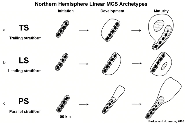
Linear MCSs also have leading stratiform (LS) and parallel stratiform (PS) structures (Fig. 7.90). Although the three modes were identified from midlatitude systems, they are still applicable to the tropics. The LS and PS types are less common but are significant in monsoon areas of Southeast Asia, where they occur along the Mei-yu/Baiu front.
In prevailing easterly winds, tropical squall clusters move rapidly westward as a continuous disturbance or family of regenerating systems that undergoes decay and regeneration over several days.227 Some squall clusters in West Africa appear quasi-circular from an IR satellite perspective but most have a leading line/trailing stratiform precipitation structure.228 Amazon squall lines, meanwhile, tend to elongate over time reaching 1000-2000 km along the leading line. Table 7.3 compares the size, duration, displacement, and propagating characteristics of squall line populations in West Africa and the Eastern Atlantic with those in South America. Amazon squall lines occur about every two days and are most common during April to June and least frequent during October and November.229
| Region | Average Propagating Speed (ms-1) |
Lifetime (h) |
Average Displacement (km) |
Length (km) |
Width (km) |
| West Africa | 14.8 | 39.7 | 2100 | 750 | 433 |
| Amazon coastal squall line |
16 | 16 | 2000 | 1400 | 170 |
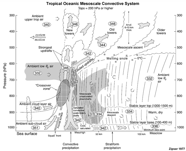
Tropical squall line passage is marked by a distinct roll cloud followed by a sudden wind squall then a heavy downpour that usually lasts about half an hour. The vigorous convection is then followed by lighter stratiform rainfall, which continues for many hours and comprise about 40% of the MCS total precipitation. Below the melting level (indicated by the bright band in Fig. 7.89), evaporative cooling of precipitation drives mesoscale downdrafts in the wake of the intense convection (Fig. 7.91). The moist static energy decreases with the passage of the leading convective line and gradually increases in the wake of the convection (Fig. 5.19). The lifecycle of a tropical squall line with trailing stratiform region is illustrated and described in Box 5-4Box 5-4.
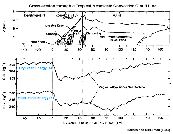
Bow Echo
The bow-echo is a subset of squall line MCSs. When a line of strong convective cells or a single large convective cell evolves into an arc shaped MCS, it is known as bow echo because of its bow shape on radar displays. The typical radar echoes observed during the lifecycle of a bow echo is shown in Fig. 7.92, a pattern observed in single cells or squall lines of 100s of km.
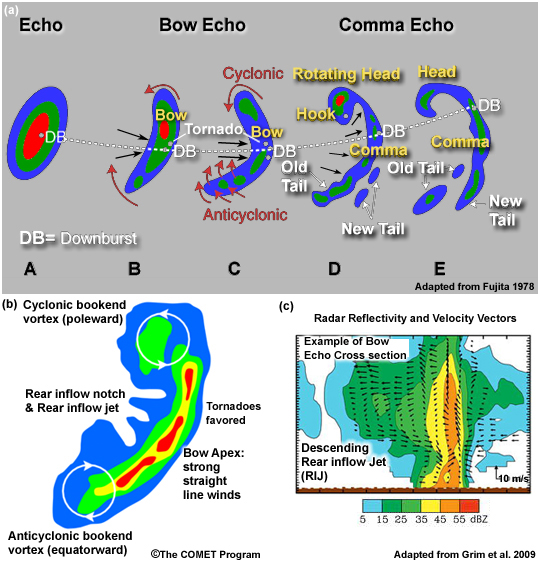
Prominent in bow echoes is a strong Rear Inflow Jet (RIJ, Fig. 7.92c), whose descent tends to produce damaging surface winds, and a rear-inflow notch (an area of weak reflectivity) that is often seen just before and during the formation of the bow (Fig. 7.92b).234 Vortices, known as bookend vortices, form on the ends of the convective line. In long-lived bow echoes, the Coriolis force promotes stronger cyclonic shear behind the poleward end of the bow and weak anticyclonic shear equatorward of the bow (Fig. 7.92b).
Mesoscale Convective Complex (MCC)
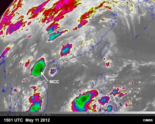
The MCC is a special case of MCS, noted for its quasi-circular, long-lasting, extremely cold cloud tops (Fig. 7.93). It is a large meso-α-scalemeso-α-scale convective system that meets size, shape, and duration criteria based on infrared satellite data235 (Table 7.4). Note that the precipitation structure of MCCs is not distinctly different from other large MCSs. The association of MCCs with devastating flash floods has been recognized since the late 1970s.236 Although it does not describe all "MCC-type" systems, the definition succeeds in identifying the largest, long-lived convective systems that are important for hydrometeorological purposes. MCCs exhibit mean cloud shield areas of 350,000 km2 and persist for an average of 11h. Oceanic MCCs are, on average, slightly larger and longer lasting.
| Size | (A) Cloud shield with IR temperature ≤ -32° C must have an area ≥ 100,000 km2 (B) Cloud shield with IR temperature ≤ -54° C must have an area ≥ 50,000 km2 |
| Initiate | Size definitions A and B are first satisfied |
| Duration | Size definitions A and B must be met for a period ≥ 6 h |
| Maximum Extent |
Continuous cold cloud shield (IR temperature ≤ -32° C) reaches maximum size |
| Shape | Eccentricity (minor axis/major axis) ≥ 0.7 a time of maximum extent |
| Termination | Size definitions A and B no longer satisfied |
Like other MCSs, convection begins in the late afternoon and peak precipitation rates (over 25mm h-1) occur in the 2-6h period after initiation.237,238 A meso-β-scalemeso-β-scale convective scale growth cycle within the first three hours seems to distinguish the relatively long lived MCCs from shorter lived MCSs. As the MCC matures, the total rain rate decreases, becomes more stratiform, as the rain area expands. Stratiform rainfall is 30-40% of the system total. After 10-12 hours, rainfall ends and deep convection ceases in the early-to-late morning.
Three distinct circulations are found in mature MCCs and other large MCSs:
- a large, cold and shallow anticyclone in the vicinity of the tropopause,
- a boundary layer cold mesohigh, and,
- in the midlevels, strong latent heating, convergence and a mesoscale updraft.
Near maximum mean upward motion, upper tropospheric divergence, and vorticity occur throughout the mature stage and is maintained through the decay stage. The decaying MCC leaves significantly amplified mid-level convergence and vorticity; at the upper-levels it leaves an anomalous upper-tropospheric high and wind perturbations extending beyond the MCC boundary. Thus, MCCs have the ability to attain inertial stability and last for more than a diurnal cycle and influence the large-scale environment in which they form.
Non-squall Tropical Cloud Clusters
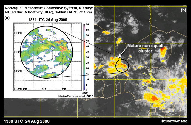
While squall lines have distinctive linear structure, non-squall tropical cloud clusters are less organized, appear amorphous in radar images, and move more slowly (Fig. 7.94). They occur more frequently than squall clusters, possess more varied precipitation structures but their precipitation rates are similar to squall lines/clusters. The large-stratiform anvil of tropical non-squall clusters sometimes meets the MCC criteria.
Diurnal Cycle
The general lifecycle of MCSs is influenced by the diurnal cycle and modulated by elevated terrain, coastal topography, and the large-scale environment.81,239 The most intense convective precipitation features (defined by ice scattering) peak around 1500 local time (LT).240,241,242 However, most tropical MCSs reach their maximum between midnight and 0300 LT242 (Fig. 5.44). Satellite cold cloud perspective shows a similarly nocturnal lifecycle for large MCSs. Unlike individual thunderstorms, MCSs develop mesoscale circulations that may become inertially-stable, i.e., balanced relative to the Coriolis Effect and able to sustain themselves for more than one diurnal cycle. In some regions, the diurnal cycle of MCSs is coincident with the evolution of a nocturnal low-level jet, which supplies the MCSs with moist air during nighttime.
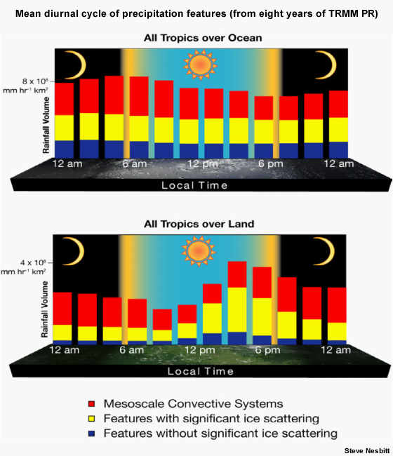
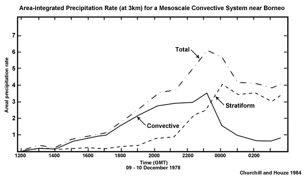
Early in the lifecycle and in the afternoon to evening, convective precipitation dominates. As the MCS matures, the total rain rate decreases, becomes more stratiform, as the rain area expands. Stratiform rainfall is 30-50% of the system total (e.g., Fig. 7.95).
Oceanic MCSs reach their peak intensity in the early morning,242 for reasons that are remain debatable.244 One early hypothesis for the overnight growth holds that horizontal divergence due to differential radiative heating near tropical cloud clusters can lead to mass circulation that enhances cloud development.245 Another theory suggests that overnight longwave cooling at the cloud top and warming at cloud base leads to destabilization and increased convection.246,247 A third mechanism holds that with longwave cooling, relative humidity increases sufficiently that entrainments effects are diminished, which benefits cloud development.248,249 A fourth mechanism explains the 2-day cycle in mesoscale convection over tropical oceans. It considers the variations in the near surface layer and its evolution in response to deep convection.250,251 During the afternoon, the warm ocean surface initiates new convection, which reaches maturity in the nighttime. Then, the next day, deep convection is inhibited as the near surface layer is stabilized in the wake of the MCS precipitation and the ocean is shaded by the remnant cloud shield.
The MCS diurnal cycle is also influenced by whether the monsoon is in "active" or "break""active" or "break" mode. For example, during the active monsoon when deep zonal westerlies dominate over northern Australia, MCSs reach their maximum area in the late morning, a characteristic that is more typical for maritime convection. While during the break phase, when zonal flow is easterly, the MCS areal extent peaks in the early afternoon, which is more typical for convection over land.252,253
7.2 Mesoscale Weather Systems »
7.2.2 Mesoscale Convective Systems »
7.2.2.3 Environments of Tropical MCSs
Vertical Wind Shear
While the main ingredient for cumulus convection is moist air that is warmer than its environment (Section 5.2.2.2Section 5.2.2.2), the vertical wind shear is critical for determining the organizational mode and longevity of MCSs.234,254,255 The CAPE is key to their updraft strength and depth.256
Tropical versus Midlatitude Shear
In general, tropical MCSs develop in environments with weaker cold pools and weaker horizontal wind shear than the midlatitudes. Both tropical and midlatitude MCSs have weak or straight-line mid-level shear profile with most of the vertical wind shear found in the low-levels (often generated by a low-level jet). The 950 and 650 hPa shear in non-squall tropical clusters (the least intense MCSs) is less than 5 m s-1 while tropical squall lines with bow echoes (which have the highest likelihood of strong, straight-line surface winds) have mean shear of about 13 m s-1. By comparison, 10 m s-1 is the upper threshold for weak shear environments in midlatitude MCSs.
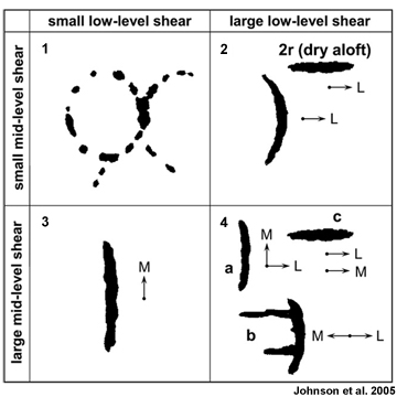
Figure 7.96 shows how shear organizes tropical convective structure and orientation, with lines generally perpendicular or parallel to the shear in the low and mid-troposphere.257,258 With weakly sheared environment, convection developed along outflow boundaries (Panel 1), With strong low-level shear and weak midlevel shear, the main convective band is perpendicular to the low-level shear (Panel 2 in Fig. 7.96). Without strong low-level shear, lines form parallel to the low-level shear (Panel 3), while more complex structures occur with strong low and mid-level shear (Panel 4).
Updrafts in MCSs
In MCSs with a trailing stratiform region, updraft speeds range from 5-17 m s-1 in the convective region and 35-45 cm s-1 in the stratiform region. Mesoscale downdrafts, in the stratiform region, of the typical tropical MCS are in the 5-25 cm s-1 range. How do these MCS features form and evolve?
1) The traditional view is of updrafts created because of static instability, also known as buoyant or gravitational instability. Parcels of warm, moist (with high equivalent potential temperature θe) air from the boundary layer, accelerate upward after being forced above the local level of free convectionlevel of free convection, entrain varying amounts of environmental air via in-cloud turbulence as they rise, then decelerate and eventually stop and spread out laterally at or near the equilibrium level, where they are neutrally buoyant (Section 5.2.2.2Section 5.2.2.2). However, the idea undiluted updrafts in hot towers over the oceanic equatorial trough has been challenged by recent field and satellite observations.259 Such undiluted updrafts are relatively rare over tropical oceans; rather, freezing is an important source of additional buoyancy.25
2) The upward air motion that maintains a mature MCS occurs in the form of a deep slantwise ascending layer of air.260 In this view, θe is conserved along streamlines.261,262 If the large-scale environment is unstably stratified and sheared, air must flow through the storm along a unique set of streamlines. For a typical environment of strong low level shear, the updraft would then be of a layer ascending on a slantwise path through the storm.
3) Another theory is that of gravity wave responses to the heating by the MCS.263,264 Simulations of MCSs found that once convective cells become clustered into an organized mesoscale group, this structure serves as a quasi-steady heat source. A layer of 3- to -6 km inflow is then drawn up through the system as a gravity wave response to the heating. The layer of inflow air enters the convective region, rising and exiting as the middle to upper level front-to-rear flow.
4) Moist absolutely unstable layer (MAUL) layer lifting operates when the layer is potentially unstable265 (Fig. 7.97). Radar observations of MCSs during TOGA-COARE showed sloping updrafts with finite layers of air, 0.5-4.5 km depth, rising over a downdraft cold pool.266
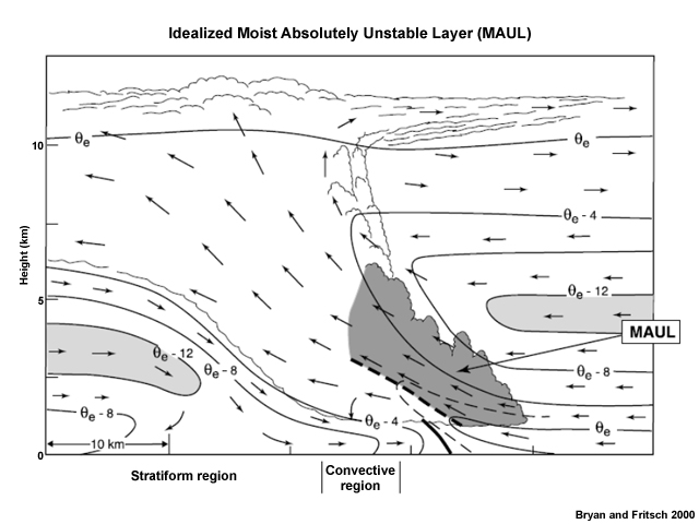
Thermodynamic evolution
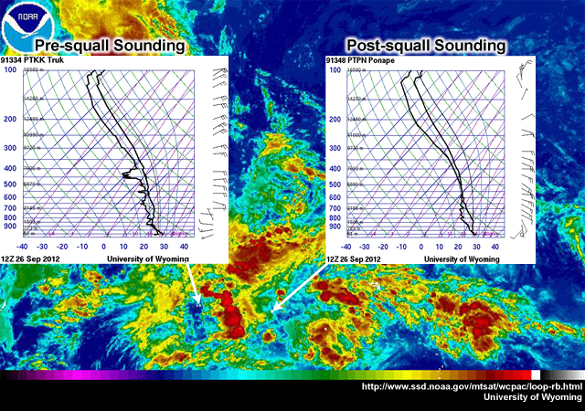
The pre-squall environment is marked by a moist boundary layer, moderate-high CAPE, low level of free convection (Fig. 7.98). As the squall line passes, the following features are observed: a pre-squall mesolow (due to subsidence warming in the mid-to upper troposphere), a mesohigh (due to heavy precipitation and convective-scale downdrafts), and a wake low (due to subsidence warming and as a surface expression of the descending rear inflow jet) (Fig. 5.19). Post squall environments are characterized by subsidence, adiabatic compression, which warms and dries the lower troposphere, as indicated by an onion-shaped sounding231 (Fig. 7.98). A squall line example is shown but the process is similar for other MCSs.
Squall Line MCS environments
Tropical squall line development is aided by strong low-level wind shear (for GATE squall lines, the critical threshold was 13 m s-1 in the 950-650 hPa layer, mostly perpendicular to the leading line). Squall lines, in turn, transport momentum upgradient, increasing the low-level vertical wind shear.
The organizational mode of the squall line, e.g., its slope and size of the stratiform region, is dependent on the relative strengths of the downdraft-generated cold pool and the vertical wind shear.254,255,267 The strength of the cold pool influences its propagation speed. The convectively-generated cold pool acts as a gravity current because it is denser than its environment. New convection is formed by uplift along the boundary of the cold pool. Its speed is given by:
 (4)
(4)where h is the height of the spreading cold pool, g is the gravitational constant,  is the environmental virtual potential temperature and
  is the perturbation virtual potential temperature of the cold pool. Gust fronts can precede storm cells of a few tens of km (20 to 40 km). Normally, the density current head has a rotor circulation. The typical depth of the cold pool is ~ 1 km. It is often thinner over the ocean (200-300 m) than over continents (up to 3 km). With passage of the cold pool, winds intensify and rotate, temperature drops 2 to 10° C, and pressure jumps 1 to 2 hPa. The moisture content also falls.
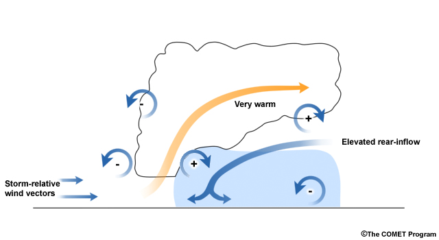
When the shear is stronger than the cold pool, the updraft is tilted away from its source of warm, moist air and the tops of the cells are shorn off. When vertical shear is weak, the cold pool moves out from the original updraft, cutting off the supply of warm, moist air (the high θe air). When the shear vorticity is balanced by the cold pool vorticity, the updraft remains upright, the cold pool triggers lifting, and the convective system is long-lived254,255 (Fig. 7.99).
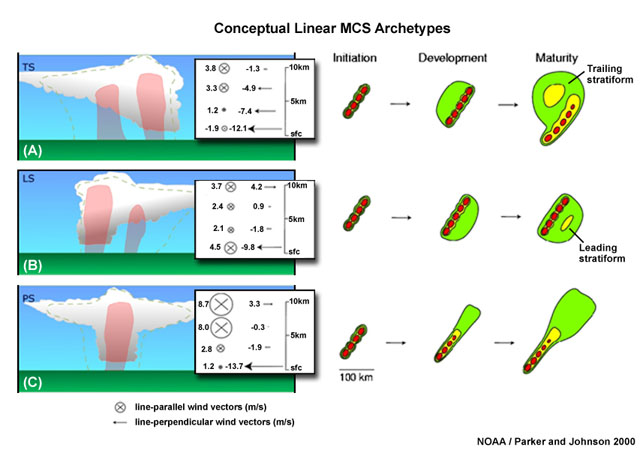
How the stratiform region evolves reflects the orientation of the vertical shear vector relative to the squall line motion (Fig. 7.100). The commonly observed trailing stratiform type develops where dominant shear is perpendicular to the line. The parallel stratiform region has more line parallel shear in the upper-levels and the leading stratiform has weaker low-level shear than the other two types (Fig. 7.100). It is not clear how the archetypes can be applied generally in the tropics given the generally weaker shear compared with the midlatitudes.
At the large-scale, the dominant forcing of squall clusters in the western Pacific and tropical Atlantic is convergence in the ITCZ. Systems observed during the Global Atmospheric Research Program (GARP) Atlantic Tropical Experiment (GATE) formed several hours after large-scale convergence was established and moisture flux increased in the low-middle troposphere.
Squall clusters also occur with easterly waves, which are noted for having low-level convergence, divergence above 200 hPa, and non-divergence in between. They normally form ahead of the easterly wave trough, move at about twice the speed of the wave, and tend to die just behind the ridge. Amazon squall lines have added mesoscale forcing from the sea breeze front.48,268
Bow echo environments
Bow echoes most commonly occur in an environment with strong deep layer shear in combination with high CAPE, steep midlevel lapse rates, and a strong cold pool. Bow echoes sometimes develop within pre-frontal squall lines and tropical cyclone rainbands. For example, squall lines and bow echoes in the developing Tropical Storm Nicole (2010) produced tornadoes, damaging strong surface winds, and heavy rainfall (COMET module, Severe Weather and Flooding in Jamaica, http://www.meted.ucar.edu/radar/tropical_cases/navmenu.php?tab=2&page=1.0.0).
MCC environments
Most MCCs initiate within prominent baroclinic zones (such as the monsoon trough, stationary fronts, and the Mei-Yu/Baiu front), which have locally large values of lower-tropospheric vertical wind shear and CAPE. Development is favored when a convectively-generated surface cold pool combined with substantial low-level vertical wind shear leads to a deep layer of slantwise ascent and a large stratiform cloud region. Most of the wind shear in MCC environments is found in the low-levels (often generated by a low-level jet).
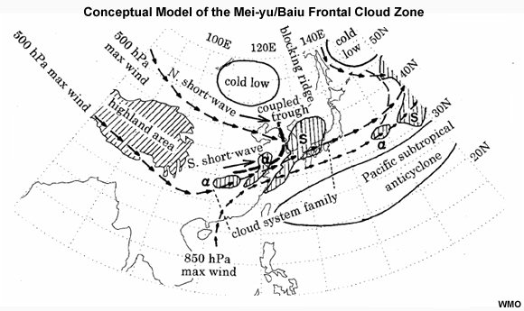
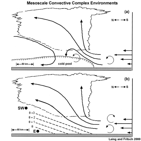
MCC formation can happen with or without large-scale forcing (Fig. 7.101). If the sign of cold-pool-induced circulation is always the same as that associated with the ambient shear then the convection will be long-lived. This secondary mechanism (Fig. 7.101b) is likely in Northern Australia MCCs that have weak baroclinic forcing. In that region, MCCs are associated with the monsoon trough and are often precursors to tropical cyclones.
Large-scale environments conducive to MCCs usually have: a low-level jet of air with low static stability, high equivalent potential temperature (θe), oriented nearly perpendicular to the baroclinic zone, flowing towards the genesis region, and is forced to rise over a relatively shallow, surface-based layer of relatively cool air.235,239 The surface cool layer is overlaid by pronounced warm advection accompanied by strong lower-tropospheric veering. A local maximum in absolute humidity and a local minimum in static stability favored MCC initiation. Low-level convergence, upper-level divergence, and a mid-level vorticity maximum, and weak mid-level shear are also characteristic of the mean genesis environment. West of Borneo in the Maritime Continent is a common location for MCCs.269,270
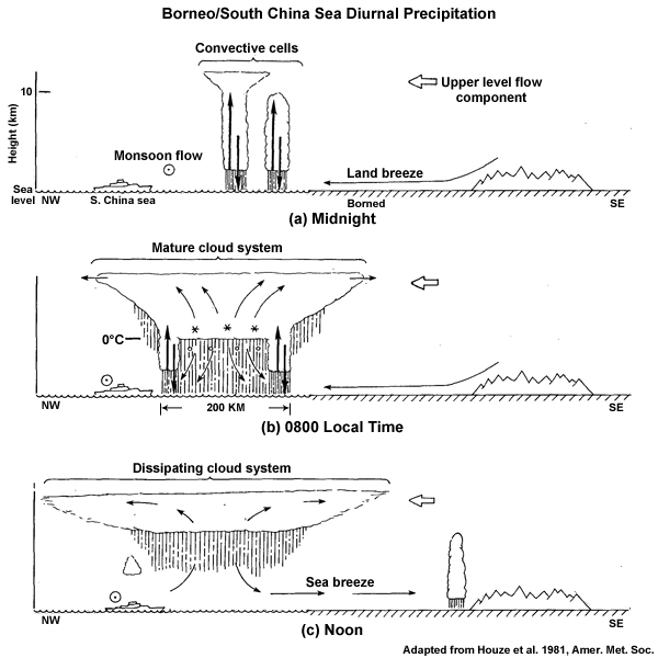
There, favorable strong low-level convergence and low-level wind shear are produced from the interaction of northeast monsoon winds and the sea breeze269 (Fig. 7.102).271 MCCs also form along the shores of northwest South America, where initial thunderstorms develop along the mountain slopes in response to diurnal heating of elevated terrain. Then it is suggested that thermally-forced gravity waves propagate offshore and initiate MCCs during the nighttime.271
Non-squall cluster environment
A distinctive feature of non-squall cluster environments is the absence of strong shear between 700 and 250 hPa. They have deep layer moisture and maximum low-level convergence during the growing stage of the system lifecycle. Maximum vertical motion is close to 300 hPa and occurs during the mature phase.
During GATE, clusters formed where the mean 950-650 hPa environmental shear was about 6 m s-1 and mostly parallel to the lines. Non-squall clusters are similar to squall clusters in terms of conditional instability and formation relative to the African easterly wave trough. However, large, longer-lived non-squall clusters tend to move at less than the speed of the easterly wave and dissipate once they fall behind the trough axis. Similar winter monsoon clusters near Borneo are initiated from offshore breezes and a quasi-stationary vortex that develops cross-equatorial monsoon flow (Section 3.5.3Section 3.5.3).
7.2 Mesoscale Weather Systems »
7.2.2 Mesoscale Convective Systems »
7.2.2.4 MCS Propagation
MCSs propagate and remain coherent via a number of methods: discrete propagation along outflows from baroclinic boundary circulations, low-level jet processes, gravity-wave interactions, and other larger-scale forcing mechanisms.272 Both tropical and midlatitude MCSs initially propagate with the synoptic-scale flow. MCS motion will follow the synoptic flow until a significant cold pool develops, which is almost coincident with the forming of the MCS stratiform anvil.
Propagation by cold pool dynamics entails the merging of cold pools generated by MCSs into a mesoscale cold pool. This larger cold pool then acts as a gravity current and lifts unstable air upward, thereby generating new convection on the leading edge of the MCS.
Discrete propagation is another suggested mechanism. Once the cold pool is established, it is important to understand the low-level jet (a prominent feature in MCC environments) in order to predict the system motion. The low-level jet is a narrow band of strong winds at or near 2-3 km above the ground. Some are nocturnal jets that persist into the morning273 and others are seasonal or synoptically forced. Areas of prominent low-level jets (solid blue shade) around the globe and associated regions of MCS activity (dashed boxes) are shown in Fig. 7.103. A new line of convection will form some distance from the MCS cold pool, towards the region of the low-level jet,274 which provides the moist air for maintenance of the MCS.
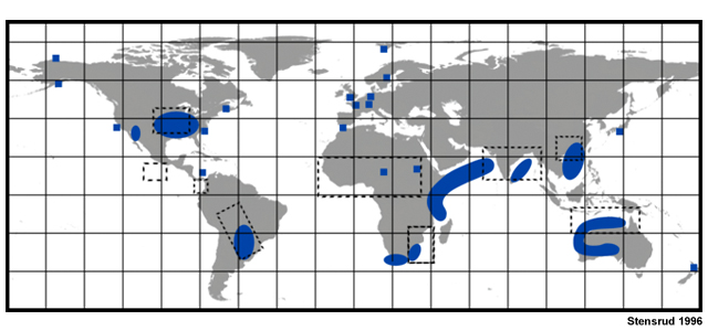
7.2 Mesoscale Weather Systems »
7.2.2 Mesoscale Convective Systems »
7.2.2.5 MCS Interaction with Large-scale Tropical Circulations
Tropical MCSs are modulated by large-scale circulations such as easterly waveseasterly waves, equatorial waves,81,276,277 and the MJO.277 The dominant forcing of squall clusters in the tropical regions of the western Pacific, West Africa, South America, and Atlantic is convergence associated with the ITCZ. Systems observed during GATE formed several hours after large-scale convergence was established and moisture flux increased in the low-middle troposphere. Although African easterly wave troughs (AEWs) provide favorably large-scale dynamic environment for enhancement of MCS precipitation, only 30-40% of West African MCSs are associated with AEWs. The variability of MCSs has more to do with regional thermodynamics, such as CAPE, convection initiated by elevated heating, and dynamics (e.g., low-level shear maxima) rather than enhancements due to the AEW regime.45,49,278

Kelvin waves, which move eastward along the equator, are noted for having large and more intense MCSs within their wet phase and very little organized convection during the dry phase. Figure 7.104 shows where the passage of a Kelvin wave across equatorial Africa leads to the formation of MCSs with extensive cold cloud areas during the wet phase and a period of little organized convection during its dry phase. Notice that the MCSs are forming each day within the Kelvin wave envelope. Similarly, the planetary scale MJO, also affects the propagation and organization of MCSs and other convective systems.
Conversely, mesoscale convection affects the large-scale systems through heat, moisture, and momentum transport. Long-lived MCSs are an important link between the convective and large-scale atmospheric circulation because they modify the vertical distribution of heating and moisture.
7.2 Mesoscale Weather Systems »
7.2.2 Mesoscale Convective Systems »
7.2.2.6 Global Distribution and Impacts
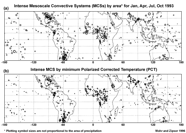
According to observations from the Special Sensor Microwave Imager (SSM/I) satellite, intense MCSs are most prevalent over tropical South America, tropical Africa, and the oceanic warm pool. They are 35% more frequent over the oceans at sunrise than at sunset and 60% more frequent over continents at sunset than at sunrise. Except over subtropical oceans, MCSs are larger at sunrise than at sunset. The total population forms a continuous, approximately log normal, distribution with the frequency inversely proportional to the area and intensity. No significant relationship was found between size and intensity. Intense MCSs which accounted for only 4% of that database, were mainly continental and more occurred in the subtropics than in the tropics (Fig. 7.105). The largest and coldest of the intense MCSs occurred over US Gulf Coast, the South American Plains, and northern India/Bangladesh, areas also favored for MCC formation. More recent climatologies from the TRMM satellite have found similar characteristics.209,210
Societal Impacts
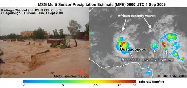
MCS rainfall is beneficial for agriculture during the growing season but is also often hazardous because they cause devastating flash floods (e.g., Fig. 7.106).
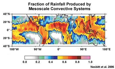
For the global tropics, they produce more than 50% of the rainfall in heavily raining areas (where the average annual rainfall is greater than 3 mm day-1). MCSs produce as much as 90% of rainfall in certain land areas. They are the main precipitation source in the semi-arid African Sahel57,280 (Fig. 7.107). Over the western Amazon, large MCSs comprise a small fraction of convective systems but they contribute most of the cloud cover and precipitation.281 On average, MCSs over land have higher rain rates (6 mm h-1 maximum) than oceanic MCSs (~ 4 mm h-1 maximum).282 In 2009, the maximum amount of rain in tropical MCSs occurred over the Bay of Bengal and off the coast of Colombia (> 20 mm per day).282
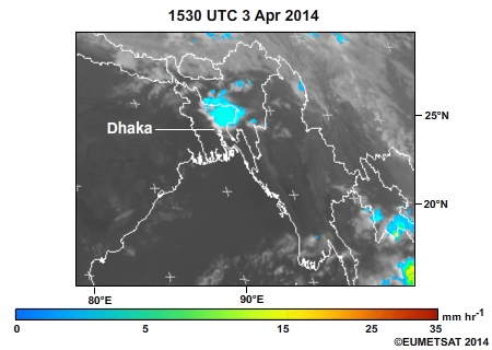
MCSs are associated with numerous hazards including damaging winds, heavy rainfall and flash floods, hail (Fig. 7.108), and tornadoes. The severity and types of hazard depends on the organization mode of the MCS.
- Tropical squall line: Tropical squall MCSs produce frequent lightning, heavy rainfall (often in excess of 25 mm h-1), flash floods, strong winds, microbursts (mostly non-severe), hail (mostly small < 20 mm), and occasional supercell, and non-supercell tornadoes and waterspouts.
- Bow Echo: Bow echoes are noted for causing damaging straight line surface winds, along the bow axis, called derechos. Derechos are defined as a family of downburst clusters with winds exceeding 33 m s-1 (64 kts) across an area whose major axis is at least 400 km. Large MCSs can produce multiple bow echoes and derechos. Tornadoes can form near the apex of the bow on the poleward side of the bow.
- MCCs: MCCs are most famous for producing heavy rainfall and flash floods. The heaviest rainfall generally occurs during the early growth stage. The MCC initiation period is also when most of the severe weather (high wind, tornadoes and hail) occurs in MCCs283 over the US. In the US, MCCs produce about half the number of severe weather events as linear MCS (squall lines).284 It is not known if similar percentages occur in the tropics.
- Non-squall clusters: Their main impact is on precipitation as they are slower moving; producing fewer severe weather than other MCSs.
MCSs are also an important source of turbulence, specifically:
- Convectively induced turbulence (CIT), which occurs within deep convective clouds, updrafts, downdrafts, and thunderstorm anvils.
- Near-cloud turbulence (NCT) in the285 clear air around the MCS, due to gravity waves propagating from the MCS, unstable upper-level storm outflow, and cirrus cloud bands.
7.2 Mesoscale Weather Systems »
7.2.2 Mesoscale Convective Systems »
7.2.2.7 Heat and Moisture Transport
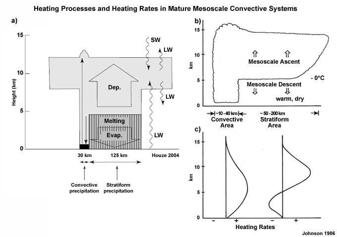
Convection has a greater impact on the large-scale when organized into mesoscale systems than as individual thunderstorms. This is particularly evident in the vertical distribution of heating due to latent heat and radiation (Fig. 7.109) in the convective and stratiform regions of MCSs. About 50% of tropical rainfall is due to MCSs,210 which means that they modulate the radiative heating balance, influence the large-scale circulation, and the distribution of moisture.
In order to quantify the vertical transport of heat and moisture, it helps to consider an ensemble of cumulus clouds embedded in a large-scale circulation.262 The heat and moisture budget can be expressed as:
 (5)
(5)where QR is the net radiative heating, Q1 and Q2 are the residuals of heat and moisture budgets of the resolvable motion called the apparent heat source and moisture sink, respectively, by Yanai et al. (1973).288 The heat budget can be divided into its cumulus/convective (Q1c, Q2c) and mesoscale stratiform (Q1m, Q2m) components:
 (6)
(6) (7)
(7)The stratiform precipitation exerts great influence on the overall vertical heating profile. The intense but smaller convective region has updrafts from the boundary layer up to the equilibrium level and precipitation downdrafts only in its lowest levels. Net heating results from latent heat released during condensation (Fig. 7.108a). In contrast, the stratiform region has a large region of ascent, from layer lifting and older updraft elements spreading out from the convective region, and downdrafts below the melting layer. The resulting stratiform profile has warming above and cooling below due to melting and evaporation beneath cloud base (Fig. 7.108b,c). The arrangement of convective and stratiform regions means that the net MCS heating is concentrated in the middle to upper troposphere.
The larger the percentage of stratiform region in an MCS, the higher the level of maximum heating. The heating profile will also be affected by the relative amounts of shallow versus deep convection present in the MCS. Therefore it is not surprising to find out that heating profiles vary among regions. Midlatitude MCSs generally have a sharper peak in heating and at a higher level than tropical MCSs. Maximum heating in western Pacific MCSs occurs in the mid-upper levels during the mature-to-decaying stages while GATE systems experience maximum heating earlier and in the lower troposphere.289
Radiative Balance
One of the most important aspects of deep convection is its influence on the tropospheric radiation budget. Tropical mean humidity and radiative fluxes are dependent on the degree of convective aggregation.290,291 The distribution and characteristics of hydrometeors and other cloud particles determine the radiation balance. Because the stratiform region of MCSs is broad and long lasting, it is also affected by radiative heating and cooling (Fig. 7.109a). A tropical MCS can cause net cooling from solar extinction which outweighs warming inside the system. What time of day MCSs occur can change the radiative balance. Even with constant total cloud fraction, the sign of the radiation balance is sensitive to the diurnal distribution of deep convective cloud systems.
Differential radiative heating can alter the evolution and mass circulation of individual MCSs through feedback among latent heat release, convective updrafts, and precipitation. The extensive stratiform anvil and nocturnal lifecycle of many MCSs affect the radiation balance local and regionally and may have implications for the global energy balance.
Dynamical Adjustment
Why is heating in MCSs important? The response of the atmosphere to latent heat depends on the horizontal scale of the heating relative to the Rossby radius of deformation, LR. If the horizontal scale of heating is less than LR, then most of the energy released by heating will propagate away from the disturbance as gravity waves. If the scale of the latent heating is close to or exceeds LR, then energy maintains nearly geostrophically-balanced flow. Tropical MCSs can become long-lived and influence the large-scale circulation when they are dynamically close to LR. Diabatic heating in MCSs can force upper-level jet streaks downstream by enhancing ageostrophic flow in the jet entrance. A continental-scale adjustment can favor more convection and flooding. Under certain conditions, series of MCSs regenerate, in roughly the same location and follow similar tracks, thereby aggravating their flood potential.292
7.2 Mesoscale Weather Systems »
7.2.2 Mesoscale Convective Systems »
7.2.2.8 Mesoscale Convective Vortex (MCV)
Spiral bands of midlevel clouds are sometimes observed on satellite images after the decay of the active convection in MCS. The occurrence of tropical cyclone-like structures on land has been documented since the late 1970s.
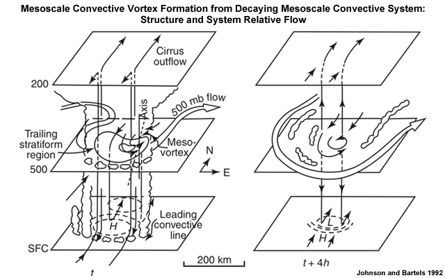
The cyclonic circulation is centered on a warm-core, mesoscale convective vortex (MCV) that sometimes develops in the mid-troposphere, in the stratiform region of MCSs228,294,295,296 (Fig. 7.110). These vortices were first noticed in tropical MCSs but have since been widely documented for warm season midlatitude continents.297,298,299
The development can be examined in terms of PV theory, which dictates that mass-integrated PV remains constant between two isentropic surfaces regardless of changes in mass transport or diabatic heating. The potential vorticity for frictionless flow can be written as:
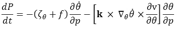 (8)
(8)where  is the diabatic heating rate, ζθ + f is the absolute vorticity on an isentropic surface, and
  is the potential vorticity.300 From the 1st term on the right, we can deduce that when diabatic heating increases with height, a positive PV anomaly will develop in the mid-troposphere. Therefore, when diabatic heating occurs in moist convection, evacuation of mass across isentropes will lead to an increase in PV, i.e., the spin of the fluid adjusts to changes in the depth of the rotating column. With saturated air in the stratiform region, the Rossby radius is smaller as the buoyancy frequency is determined by the moist static stability.286
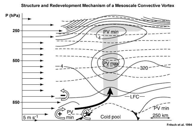
58 m s-1 and is being overtaken by air of high equivalent potential temperature in the low level jet. Air overtaking the vortex ascends isentropic surfaces, reaches its level of free convection (LFC), and thereby initiates deep convection. Shading indicates cloud.301
Most MCVs form in about six hours within an MCS of about 200-400 km in spatial extent. Then they last for 12-24 hours and decay unless convection is maintained or recurs. As a dynamical response to heating on the order of the Rossby radius, the MCV can become inertially stable (Fig. 7.111). Heating in the positive PV anomaly can persist for days, regenerating convection and amplifying the vortex.
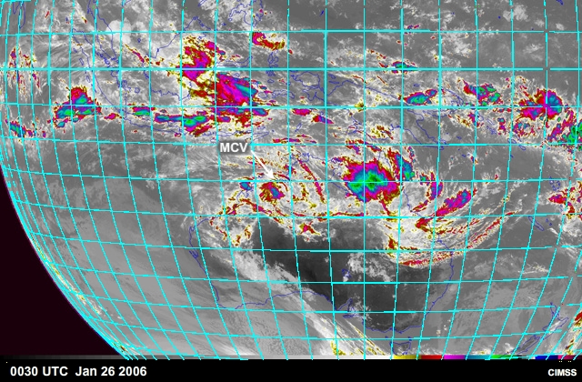
MCVs will persist in the presence of weak synoptic flow, weak vertical wind shear, and strong gradients of humidity. The example in Fig. 7.112 persisted for several days and developed into a tropical low with pressure falling to 998 hPa on 31 January. Under certain conditions, series of MCSs form, in roughly the same location and follow similar tracks, thereby aggravating their flood potential, such as occurs along the Mei-Yu/Baiu front302 (Fig. 3.39) or the South Pacific Convergence Zone (SPCZ).
Tropical cyclone effects
It has been theorized that when successive cycles of convection occur over a warm water surface, they can play a crucial role in the transition of a loosely organized cluster of convection into a tropical depression,303 provided the large-scale environment is favorable (Chapter 8, Section 8.3.Chapter 8, Section 8.3.). Tropical cyclones sometimes form when MCSs move over water, probably due to midlevel vortices extending downward. Most tropical cyclone circulations are synoptic-scale but their precipitation structure and inner core dynamics are predominantly mesoscale (Chapter 8, Section 8.4.4.6Chapter 8, Section 8.4.4.6). Satellite microwave measurements suggest that mesoscale convective bursts can lead to rapid changes in cyclone intensity and structure through latent heat feedback mechanisms.
7.2 Mesoscale Weather Systems »
7.2.2 Mesoscale Convective Systems »
7.2.2.9 Atmospheric Electrical Effects
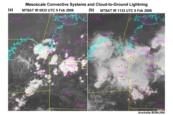
MCS are a major source of lightning. During the passage of a typical tropical squall line, the leading convection is characterized by negative cloud-to-ground (CG) lightning (Fig.7.113a). As the system matures and the stratiform region expands, large amplitude positively charged flashes become prevalent (Fig. 7.113b).
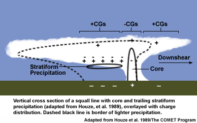
Since the early 1990s interest has grown in other electrical properties of MCSs, particularly their association with upper atmospheric transient luminous events known as sprites, blue jets, and elves.305,306 These features are observed above the stratiform precipitation region of large MCSs that favor horizontally extensive and layered regions of positive charge generation (Fig. 7.114). A necessary but not sufficient condition for sprites is an MCS with stratiform precipitation area over 20,000 km2.
The three tropical continental regions are prominent sources of lightning213,307 and sprites. Africa is the most outstanding in terms of mesoscale lightning, flashes with extraordinary energy and vertical charge that excites sprites in the mesosphere.305 West Africa has large MCSs that accumulate large amounts of positive electricity in stratiform regions in contrast the predominantly disorganized air mass thunderstorms over the Amazon. In the Congo, squall lines with large stratiform regions also have highly energetic, positive lightning and attendant sprite initiation but are less intense than MCSs in West Africa. West Africa has stronger baroclinicity, large-temperature gradients between the hot, Saharan air and the cool, moisture air to the south, compared with the more barotropic environment over the Amazon.308 Those MCSs are also longer-lived and have more large cloud condensation nuclei in the boundary layer.309
7.2 Mesoscale Weather Systems »
7.2.2 Mesoscale Convective Systems »
7.2.2.10 Chemical Transport by MCSs
Mesoscale convection is important for the transport and chemical cycling of trace gases. The convective updraft displaces the tropopause upwards leading to strong vertical mixing.310 In some tropical MCSs, overshooting convective turrets transport tropospheric air above a layer of stratospheric air. This displacement, along with a broken tropopause around the edges, injects ozone-poor tropospheric air into the stratosphere.311
Lightning in thunderstorms helps to create nitrogen oxides (NOx), primary sources of fixed nitrogen in the atmosphere that are critical to the production of tropospheric ozone, and affects the concentration of the hydroxide radical (OH) and hence can modulate oxidizing in the atmosphere. MCSs readily carry NOx to the upper troposphere, where it can remain for days312,313 and be transported over long distances, increasing the potential for ozone production in areas with limited NOx. In the Amazon Boundary Layer Experiment (1987), ozone concentrations in the mid-upper levels of squall lines were 3-4 times above background values.314 MCSs often occur in series, disturbing atmospheric thermal and trace gas fields over a large area, making them likely important local, natural source of tropospheric ozone in areas where MCSs are common.
7.2 Mesoscale Weather Systems »
7.2.3 Mesoscale and Local Circulations
In many regions of the tropics, precipitation and other significant weather are generated by mesoscale and local circulations, most of which are generated by differential heating of the earths surface and the relief of the land. For example, Fig. 7.115 shows the mean diurnal signal strength relative to the total rain. The pattern identifies regions where island and mountain effects dominate. Chapter 5, Section 5.3.7Chapter 5, Section 5.3.7, has more information about the diurnal cycle of precipitation across the global tropics during all seasons.
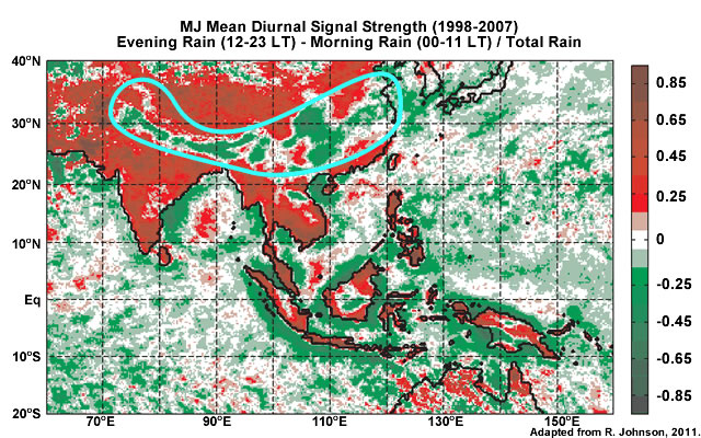
7.2 Mesoscale Weather Systems »
7.2.3 Mesoscale and Local Circulations »
7.2.3.1 Sea-Land Breeze
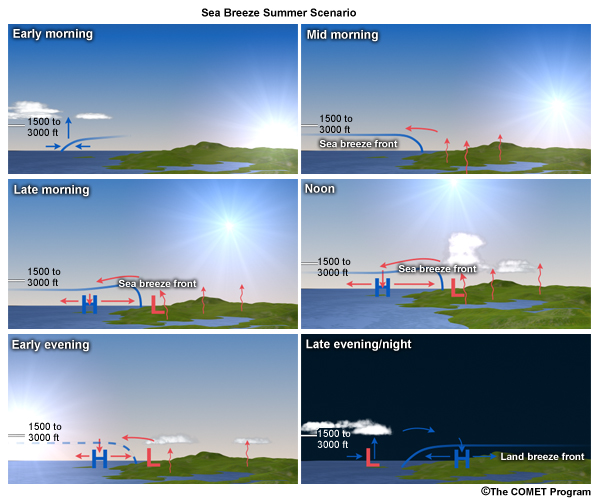
Sea and land breezes, which are among the most commonly observed local circulations, are initiated by differential heating over land and ocean (Fig. 7.116). Therefore, while tropical air masses over the ocean have slight diurnal variation, islands introduce dramatic changes in day/night cloud patterns. The daytime buildup of clouds over land is accompanied by a clear ring around the coast and offshore where high pressure dominates (Fig. 7.116). The radius of the cloud-free ring is usually comparable to the width of the island.315
The Coriolis Effect helps to constrain the horizontal effects of the land-sea breeze by turning the wind, which limits its inland-offshore influence. In the tropics, the Rossby radius of deformationRossby radius of deformation, the length scale at which rotational or Coriolis Effect become as important as buoyancy effects, is nearly an order of magnitude larger than in the midlatitudes. So a circulation such as the sea breeze can have a much larger horizontal extent in the tropics without being turned by the Coriolis acceleration.
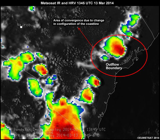
The sea-breeze flow will converge or diverge depending on the shape of the coastline. Convergence produces stronger thunderstorms, e.g., Fig. 7.117.
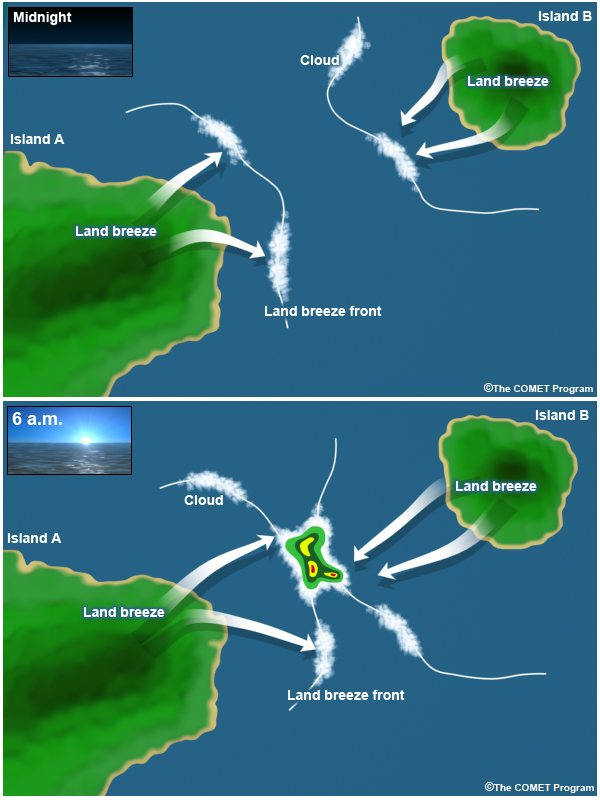
Convergence of land breezes from neighboring islands or continents can form intense thunderstorms (Fig. 7.118), common phenomena in the Maritime Continent. Even on relatively flat and small tropical islands sea breeze convergence can create intense thunderstorms, such as occurs in the Tiwi Islands, where sea-breeze thunderstorms are known as Hector. For a detailed analysis of Hector, see the Focus Section 1 of Chapter 9Focus Section 1 of Chapter 9.
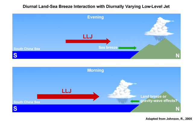
In the South China Sea, offshore thunderstorms are formed where the low-level jet converges with the land breeze or gravity waves produced by previous convection over land (Fig. 7.119).
7.2 Mesoscale Weather Systems »
7.2.3 Mesoscale and Local Circulations »
7.2.3.2 Mountain Effects
Mountain-Valley Breezes
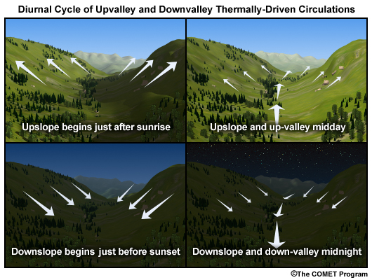
Much like the sea breeze, heterogeneous heating of the land areas with steep topography leads to mesoscale thermal circulations (Fig. 7.120). During the daytime, heating of elevated terrain leads to rising motion over the mountains, condensation, and precipitation. This sets up a circulation, known as a mountain breeze, between the mountain and the lower elevation, with low-level convergence over the mountain and divergence over lower elevation. During nighttime, the mountain areas cool and air sinks into the lower elevation, forming a valley circulation.
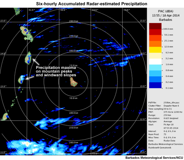
Steep terrain also serves as a lifting mechanism and a source of new convection. Therefore, the windward side of mountains will be wetter than the leeward side. For example, because of the prevailing easterly trade winds, the Eastern Caribbean islands are wet on the east and drier on the west. Accumulated precipitation maxima are aligned along the eastern mountain slopes (Fig. 7.121). Under light winds or calm conditions, convection is more centered over the high terrain.
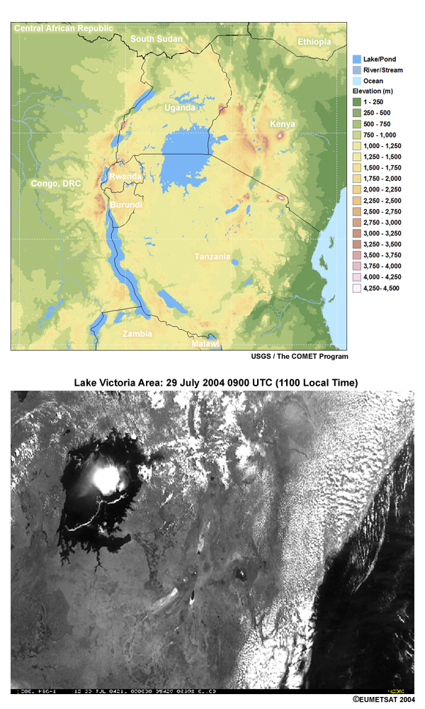
With inland lakes and mountains, local circulations are more complex. For example, the Lake Victoria area (Fig. 7.122) has both land/water and mountain/valley diurnal effects. Thunderstorms form in the convergence between the lake and mountain/valley breezes and new storms are generated along their gust fronts. On average, the diurnal cycle has thunderstorms over the eastern part of the lake during daytime and over the west during night and early morning.
Low-level Wind Maxima
Channeling of flow by high terrain creates wind maxima known as gap winds, coastal jets, and low-level jets, depending on location. Some effects are straightforward, such as the acceleration of trade winds and northers through isthmuses in the Central American Mountains.316,317
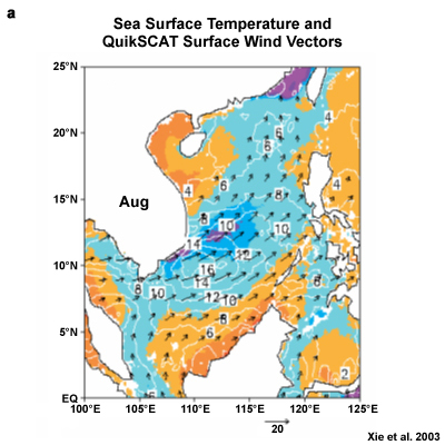
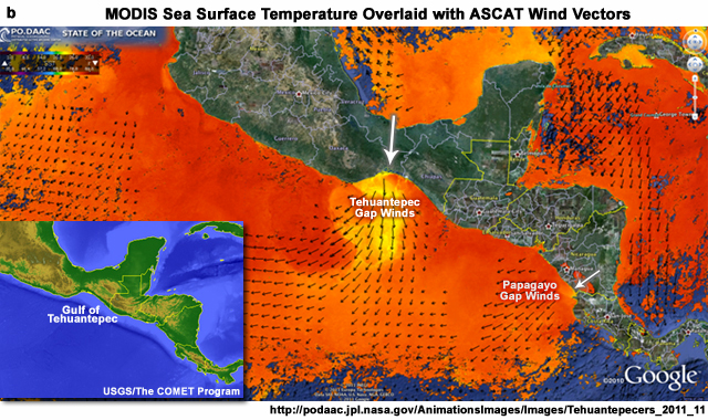
A complex topographic effect occurs along the north-south Annam Cordillera on the east coast of Indochina.318 When the southwest monsoon flow impinges on the mountain range, it creates a strong low-level jet off the coast of South Vietnam (Fig. 7.123). This causes cool upwelling that is enhanced by Ekman upwelling due to the cyclonic curl of the wind stress on the north side of the jet, leading to cooler SSTs just north of the jet axis.
Another well-known wind maximum occurs in the Gulf of Tehuantepec in southern Mexico. As northerly winds move south behind cold fronts in the Gulf of Mexico, flow accelerates through the Chivela Pass in southern Mexico leading to gale-force winds over the Gulf of Tehuantepec in the Pacific (Fig. 7.123b), causing squall lines, rough seas, and cold upwelling.319 On average about 12 gale-force and 6 storm-force events occur during October to May;320 most commonly during December and January. Higher than normal storm-force events occur during El Niño winters; not surprising given the stronger jet stream and storm tracks that are shifted southward during those episodes (COMET Module, JetstreamsJetstreams). Learn more about Tehuantepec winds in the COMET module, Forecasters' Overview of the Gulf of Mexico and Caribbean SeaForecasters' Overview of the Gulf of Mexico and Caribbean Sea.
7.2 Mesoscale Weather Systems »
7.2.3 Mesoscale and Local Circulations »
7.2.3.4 Island Circulations in the Trades and Monsoons
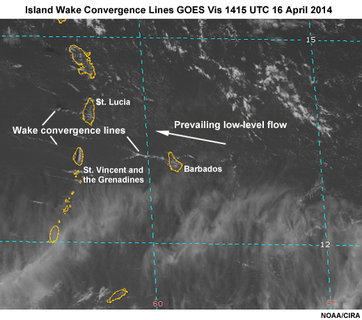
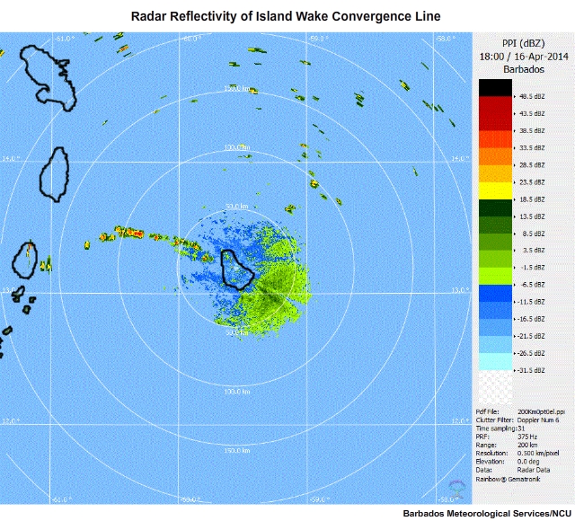
Islands disrupt the organization of tropical oceanic clouds, which typically have two dominant directional modes: cloud streets aligned parallel to the low-level wind and, less frequently, aligned at large angles to the low-level wind, but not necessarily at right angles.321 An island slows the flow causing convergence upstream, acceleration around the island, and wake vortices on the leeside.315 For example, wake vortices form downstream of the Eastern Caribbean islands as the trade wind flow merges after been forced around the islands. Convergence in the wake promotes convection and precipitation. The direction of the wake vortex depends on the direction of the trade winds. With east-or east-northeasterly winds, the wake vortex from Barbados extends to St. Vincent and the Grenadines (Fig. 7.124). When winds are southeasterly the wake vortex from Barbados extends to St. Lucia.
Another prominent example of island induced circulations is flow blocking by Taiwan during the summer monsoon. The blocked flow produces a low-level jet northwest of the island and lee vortices downstream, both of which influence where precipitation322 occurs. Similar local circulations are generated by flow around the big island of Hawaii in the north central Pacific.
7.2 Mesoscale Weather Systems »
7.2.4 Tropical Severe Weather
7.2 Mesoscale Weather Systems »
7.2.4 Tropical Severe Weather »
7.2.4.1 Ingredients for Severe Thunderstorms
While thunderstorms occur in many parts of the tropics, severe thunderstorms are rare. Severe thunderstorms, defined by the U.S. National Weather Service as producing one or more of the following: tornado; winds of at least 50 kt (25 m s-1); and hail ≥ one inch (25.4 mm) in diameter.
Why is this type of severe weather rare in the tropics? Severe thunderstorms thrive in strong vertical wind shear and horizontal gradients of moisture, temperature, and wind. Furthermore, vigorous convection that produces hail and tornadoes require dry, cool mid-levels above an inversion that caps warm, moist near surface air and lead to strong updrafts when the inversion is eroded. Temperature and moisture are fairly homogeneous in the tropical environment. Tropical updrafts are weaker than midlatitude continental updrafts, limiting hail growth, and the vortex stretching that is sufficient to produce tornadoes.
7.2 Mesoscale Weather Systems »
7.2.4 Tropical Severe Weather »
7.2.4.2 Tornadoes
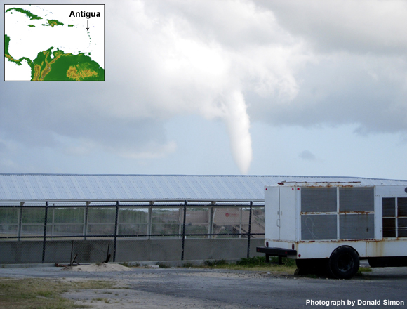
A tornado is a violently rotating column of air, extending from a cumulonimbus or cumulus congestus and reaching the surface (Fig. 7.125). It is the most destructive local scale atmospheric phenomenon.
The estimated speed of most tropical tornado vortices is less than 49 m s-1 (110 mph / 96 kts). Tornadoes last from seconds to more than an hour and their paths range from 100 m to 10s of km. They move at 5-13 m s-1 (10-30 mph/ 9-26 kts).
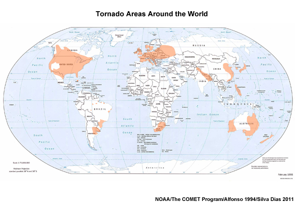
Although relatively rare, tornadoes occur on all continents except Antarctica (Fig. 7.126). They are most common in the plains of North America and Australia. Few tropical places have extensive storm-data reporting like the US. From the tropics, India recorded 42 tornadoes from 1951 to 1980 while Cuba had a mean of 41 tornadoes per year from 1981 to 1985. In Cuba and the Florida peninsula most tornadoes occur during June and July, mainly associated with waterspouts moving onshore and tropical cyclones at landfall. In India and Bangladesh tornadoes are most frequent during April and May and rarely occur during the monsoon. Strong tornadoes are most common in spring and in the late afternoon, but can occur in any season and at any time of day.
Tornado intensity is ranked by an Enhanced Fujita (EF) scale, implemented in 2007 (Table 7.5). The scale is named for Dr. Theodore Fujita who created the first tornado intensity scale in 1971. The original Fujita Scale (F scale) was based on the damage caused by a tornado. The original F-scale was limited by factors such as: categories based on the worst damage, even if done to a single structure, and failure to account for differences in construction.
| EF scale | Class | Wind speed | Description | |
| mph | km h-1 | |||
| EF0 | weak | 65-85 | 105-137 | Gale |
| EF1 | weak | 86-110 | 138-177 | Moderate |
| EF2 | strong | 111-135 | 178-217 | Significant |
| EF3 | strong | 136-165 | 218-266 | Severe |
| EF4 | violent | 166-200 | 267-322 | Devastating |
| EF5 | violent | >200 | > 322 | Incredible |
The EF scale starts with a list of 28 damage indicators that includes a description of the typical construction for that indicator category. Then the Degree of Damage is assessed and related to an expected wind speed range. Tropical tornadoes are usually weak, EF0 or EF1. Only a small percentage of tornadoes are extremely intense, EF3 or greater and they mainly occur with supercells in the midlatitudes.
Tornadoes in the tropics are typically produced by non-supercell thunderstorms, landfalling tropical cyclones, extratropical systems that extend into the tropics, subtropical lows, and hybrids of tropical and extratropical systems.
Non-supercell tornadoes
Most tropical tornadoes are weak and not produced by supercells. Non-supercell tornadoes or landspouts, are associated with mesoscale and local scale circulations in the boundary layer. The parent cloud does not have a mesocyclone as found in supercells.
The necessary conditions for the formation of non-supercell tornadoes seem to include:
(i) a lower tropospheric boundary possessing significant across-front horizontal shear,
(ii) misocyclones developing along the boundary, possibly as a result of horizontal shearing instability,
(iii) rapidly deepening moist convection along the boundary, and
(iv) an atmosphere having only weak vertical shear (compared with supercells).
As illustrated conceptually (Fig. 7.127), usually, convective cells will build and move along the boundary. When a moist convective updraft becomes co-located with a misocyclone, it becomes a tornado through vertical stretching of the vorticity along the boundary. A misocyclone, a small cyclone generated by horizontal shear instability and convergence in the boundary layer, is distinct from the larger and deeper mesocyclone, the rotating updraft in a supercell, which is due to the tilting of horizontal vorticity produced by vertical wind shear. Non-supercell tornadoes can form even when the low-tropospheric circulation is weak. Once the updraft is established, with rapid convective growth, a tornado can be produced.
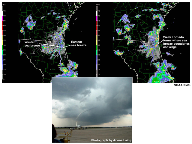
In Fig. 7.128, outflow from thunderstorms that developed along the western sea breeze and propagated east converged with the eastern sea breeze outflow. The tornado formed at the convergence zone between the two boundaries.
Supercells and Supercell Tornadoes
Supercell thunderstorms are rare in the tropics, occurring only under extraordinary conditions. However, because of their highly hazardous weather, their characteristics and conditions under which they may occur in the tropics need to be understood by tropical meteorologists. A supercell thunderstorm is an intense, relatively large thunderstorm (25-50 km scale) that produces severe weather and can last for several hours. Supercells are noted for generating the strongest tornadoes, large hail, strong winds, and heavy rain.
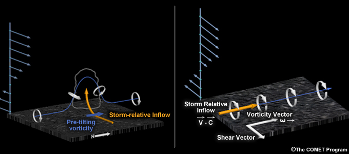
Supercells form in strongly sheared environments where the thunderstorm updraft tilts the horizontal vorticity upward to form a rotating updraft (Fig. 7.129). Environments conducive to supercell forming in the tropics occur where extratropical intrusions cause the meeting of dry, polar northerly and westerly winds with hot, moist tropical air masses, as occurs with cold fronts and subtropical cyclones. Strong shear and high CAPE are good indicators of the potential for supercells. Landfalling tropical cyclones can also generate sufficient shear to produce supercells.
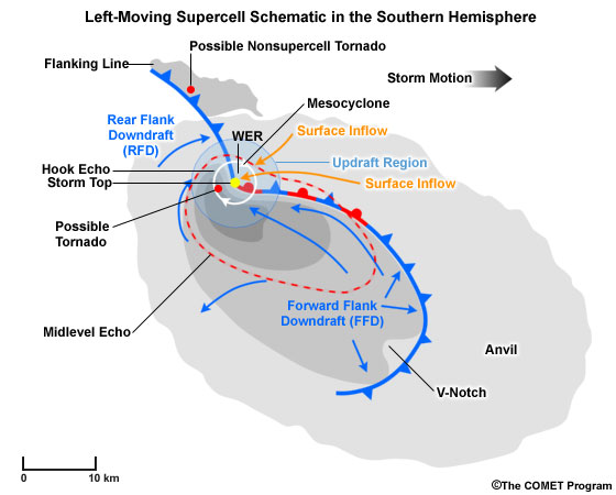
Unlike ordinary thunderstorms, supercells are characterized by a mesocyclone, a rotating updraft that is usually 2-10 km wide and about 3 km deep (Fig. 7.130). The mesocyclone creates the potential for tornado formation (white circle in Fig. 7.130) and leads to overshooting tops. A supercell generates a strong downdraft in its forward flank, where a shelf cloud spreads out and heavy precipitation usually falls. Tornadoes are also possible along the boundary created by the rear flank downdraft.

The mesocyclone is usually identified in radar base reflectivity images by a hook echo (Fig. 7.131). The hook surrounds a weak echo region where air is rising in the updraft. On base radar velocity images, the mesocyclone is identified as a rotational velocity couplet (Fig. 7.131).
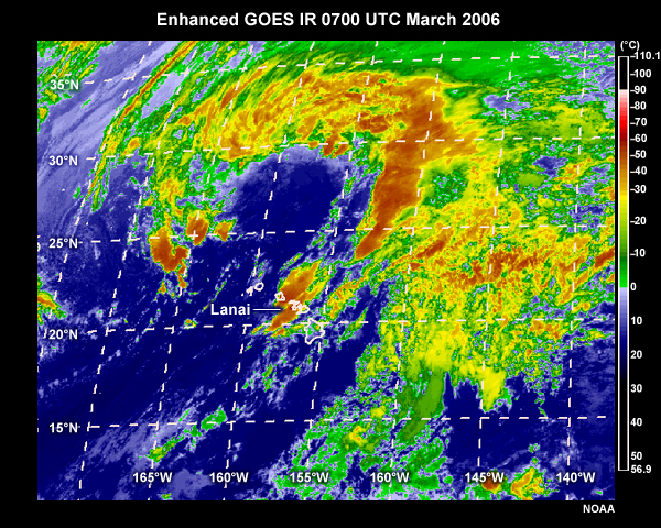
On enhanced satellite IR images, an enhanced-V or wedge-shaped cloud top feature is used to identify supercells producing imminent or current severe weather. Tornadoes and large hail usually occur near the apex of the wedge. Corresponding overshooting tops identify the same areas in high resolution visible images. Figure 7.132 shows supercell thunderstorms that produced large hail and a waterspout that moved on land in Lanai and Maui, Hawaii. The dark red areas correspond to the most intense thunderstorms; note the location of the apex of the wedge near Lanai. The vortex, seen in the radar images in Fig. 7.131, occurred about 30 minutes after the satellite image.
Tropical Cyclone Tornadoes
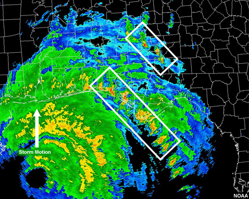
Most tornadoes spawned by tropical cyclones are weak, with intensities of F0-F2, and found in the right-forward (left-forward) quadrant of tropical cyclones in the Northern (Southern) Hemisphere (e.g., Fig. 7.133). Most are reported in the outer rainbands and commonly occur during the afternoon. The few inner region tornadoes are mostly F0 scale and have no preferential time of day.
When tropical cyclones make landfall the winds near the surface are slowed by the increase in friction and turbulence over land. This leads to lower-tropospheric vertical shear, which when tilted upwards, leads to the formation of mesocyclones. The shear over land is more than twice the shear over the ocean. From those mesocyclones tornadoes are formed and most occur when:
- The vertical wind shear from the surface to 850 hPa is greater than 20 m s-1
- The tropical cyclone is intense and/or intensifying just before landfall
Tornadoes from Extratropical Influences
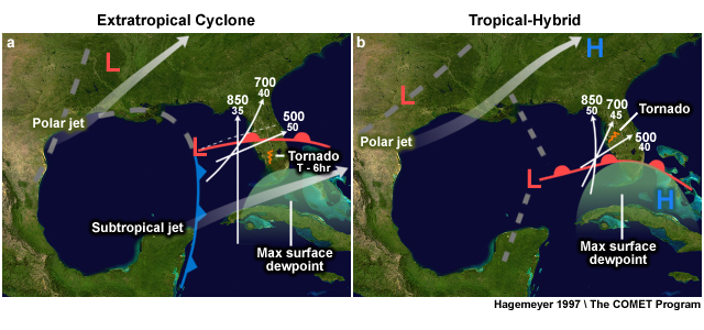
Most intense tornadoes that occur in the tropics are produced by squall lines or supercells associated with (i) extratropical cyclones or fronts and (ii) tropical-hybrid or subtropical environments (e.g., Fig. 7.134). Squall lines and supercells capable of producing tornadoes in the tropics are usually in the warm sector of extratropical cyclones, ahead of cold fronts that extend into the tropics (Fig. 7.134a). Large shear and convective instability occur when cold air from the extratropical westerlies meets warm tropical air masses flowing poleward. Such environments are conducive to the formation of severe thunderstorms, supercells, and tornadoes.
Much of our knowledge of tropical tornado environments comes from studies of tornadoes in Hawaii, the Florida peninsula, and India. According to the Florida 1950-1994 climatology,326 tornadoes from extratropical systems have environments with relatively weak instability and no capping inversion as is common in the US Great Plains. Instead, Florida extratropical tornado environments have a low-level moist layer beneath a very dry mid-tropospheric layer. The mid-troposphere dry layer comes from air subsiding in the subtropical upper-level high and acts as a source of substantial CAPE. Winds also increase with height to a maximum in the upper troposphere, where the subtropical jet promotes upper-level divergence. In Hawaii, which averages about one tornado per year, subtropical cyclones spawn thunderstorms that produce severe weather including tornadoes. Extratropical intrusions are also common in other tropical regions with reported tornadoes, such as India, Cuba, Puerto Rico, Southeast Asia, Brazil, and Australia.
Tornadoes form in a tropicalhybrid environment when tropical or subtropical lows in the lower troposphere interact with midlatitude upper-level troughs (Fig. 7.134b). The thermodynamic profile of hybrid environments is similar to the extratropical cases. However, winds weaken with height from a maximum in the lower-tropospheric to an upper-tropospheric minimum. Compared with the prefrontal more baroclinic environment, the hybrid environments are more quasi-barotropic.
7.2 Mesoscale Weather Systems »
7.2.4 Tropical Severe Weather »
7.2.4.3 Waterspouts
A waterspout is a tornado over water and is generally much weaker and narrower than the average tornado. Compared with tornadoes, waterspouts are more prevalent in the tropics and subtropics and have peak frequency in the morning and a secondary maximum in the late afternoon.
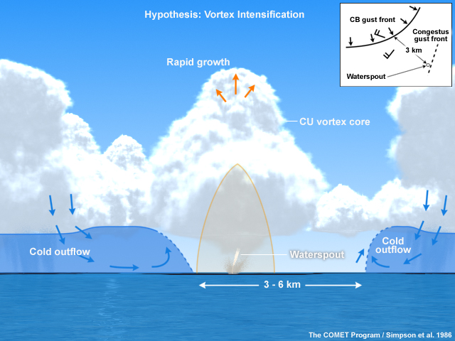
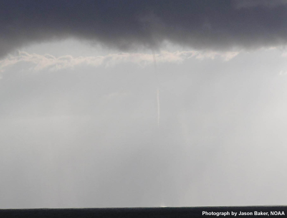
Waterspouts tend to form beneath rapidly growing cumulus congestus clouds and when cool air moves over warm water. Studies of waterspouts off the Florida coast and West Africa found that they tend to form in the convergence zone between gust fronts and where rapid convective growth is coincident with cloud mergers (Fig. 7.135).
7.2 Mesoscale Weather Systems »
7.2.4 Tropical Severe Weather »
7.2.4.4 Dust Devils
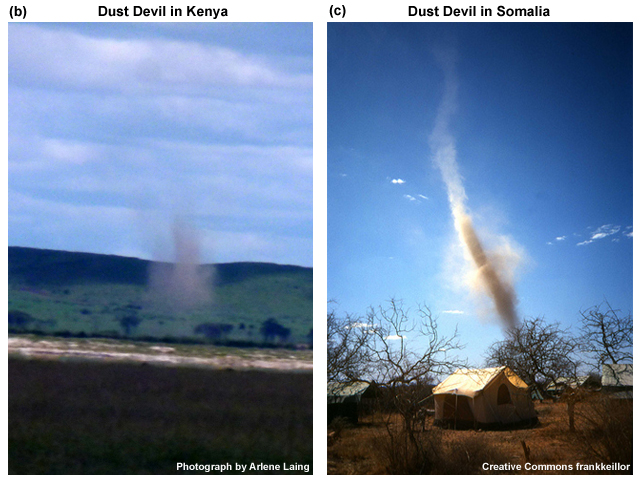
Dust devils are small vertical vortices that form in the convective boundary layer during daytime when the surface is strongly heated and the surface wind is weak (Fig. 7.136a). The dust and debris carried upward by the vortex makes it visible. They occur under clear skies or beneath a layer of fair weather cumulus and often appear in groups (Fig. 7.136b,c).
Dust devils have diameters on the order of 10s of meters and heights of 150-300 m. Most dust devils last only a few minutes but on rare occasions, they can last for an hour or more.
Summary
Synoptic and mesoscale systems account for most of the daily weather in the tropics. Unlike the midlatitudes, where synoptic weather result from baroclinic instabilities in the westerlies with energy concentrations at those scales, tropical weather has no basic current that prevails in the same manner.
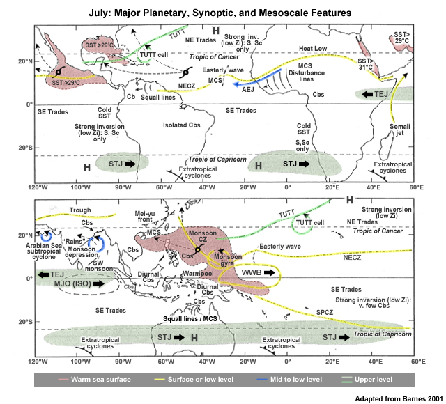
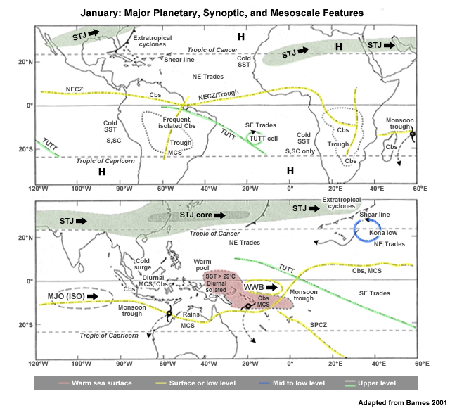
Figure 7.137 summarizes major planetary circulation and synoptic-scale features of the tropical atmosphere and associated mesoscale phenomena. While mesoscale systems form independent of synoptic features, some are modulated by larger-scale systems and circulations and mesoscale convective systems in turn modify the large-scale environment through the transport of sensible heat, moisture, and momentum.
Tropical synoptic systems are generally weaker than the midlatitude synoptic systems, with the exception of tropical cyclones. Synoptic systems in the tropics often have circulations that are prominent in about half of the tropical troposphere. For example, African easterly waves have maximum vorticity between 850 and 700 hPa, TUTTs are strongest in the upper troposphere; monsoon depressions in the Bay of Bengal are strongest below 700 hPa; and the northeast Arabian Sea has cyclones that are strongest in the mid-troposphere. All of these synoptic systems are major sources of regional precipitation and, in the case of easterly waves, subtropical cyclones, and TUTTs, contributors to the formation of tropical cyclones.
Interactions between the tropics and the extratropics are associated with Rossby wave trains that emanated from the tropics to the extratropics and vice versa. In the former case, the MJO, ENSO, and equatorial waves produce convection that perturbs the atmosphere and creates a remote dynamical response. Extratropical intrusion most often involves an amplifying Rossby wave at low-latitude that brings cool, dry air into the tropics and funnels warm, moist air into the extratropics. The latter happens most efficiently in atmospheric rivers, which are the major conduits for extreme precipitation along the western coasts at midlatitudes.
Thunderstorms are ubiquitous in the humid tropics, as they form where moist, warm air is lifted in an unstable environment. However, outside of tropical cyclones, tropical severe thunderstorms are fairly infrequent as temperature and moisture are fairly homogeneous in the tropical environment, horizontal wind shear is weak, and tropical updrafts are weaker than midlatitude continental updrafts. This limits the production of severe weather (hail, tornadoes, damaging winds).
The intensity and longevity of thunderstorms and MCSs is dependent on the vertical wind shear and structure of the system. The amount and severity of the hazards they pose increase with shear and the complexity of the storm structure, from ordinary thunderstorms with single updraft and downdraft (short-lived, usually not severe) to multicellular storms with separated updrafts and downdrafts (longer-lived, some severe weather), to complex mesoscale convective systems (damaging winds, heavy rain, flash floods, hail, occasional weak tornadoes), and supercells in landfalling hurricanes and extratropical systems at low latitudes (damaging tornadoes, occasional flash flood). Tropical MCSs are most intense over continents although oceanic systems have larger areas on average. A mesoscale convective vortex (MCV) can form in the stratiform region of large, long-lived MCS, become inertially stable, and regenerate new convection in subsequent diurnal cycles. A few MCVs have transformed into tropical cyclones.
In addition to their impact on daily weather, MCSs are also significant components of the global electrical circuit, contribute to the transport of chemicals to the upper-troposphere, and the production of nitrogen oxides and tropospheric ozone. They also modify the large-scale environment in which they develop.
Most tropical tornadoes are non-supercell tornadoes, which form most often along convergence lines in the boundary layer. Horizontal shear along the boundaries leads to the formation of misocyclones and when a thunderstorm updraft is coincident with a misocyclone, a tornado forms. Waterspouts are like weak tornadoes except for forming over water, generally warm water. They form where rapid cumulus growth is coincident with merging cloud lines and convergence along gust front. Dust devils on the other hand can form under a clear sky from air rising due to strong surface heating.
A fair amount of research is still needed to fully understand tropical synoptic and mesoscale systems and their multi-scale interactions as well as their role in high impact weather, climate variability, and air chemistry.
Questions for Review
- Describe one candidate theory for the formation of African easterly waves and explain its limitations.
- Describe the basic structure and propagation characteristics of inertia-gravity waves.
- Explain the similarities and differences between subtropical cyclones and midlatitude cyclones
- Describe the dynamical and energetic forcings that contribute to the formation of subtropical cyclones and their transition to tropical cyclones.
- Describe the structure and climatology of TUTTs and how they contribute to tropical cyclone intensity changes.
- Explain the differences between TUTT-induced lower-level troughs and easterly waves.
- Describe the differences and similarities between tropical and midlatitude squall lines.
- Describe three methods of tracking easterly waves.
- Describe how easterly waves can interact with upper-level cyclones to enhance precipitation in the subtropics and midlatitudes.
- Describe the basic structure, propagation mechanisms, and characteristic weather of monsoon depressions.
- Describe the typical lifecycle of trade wind surges and associated weather in the Atlantic.
- Explain the formation of Rossby wave trains in the tropics and their impact on midlatitude weather.
- Describe how the Subtropical Jet, the MJO, and atmospheric rivers combine to affect weather in the midlatitudes.
- Describe the influence of midlatitude cyclones, fronts, cold surges on weather in southeast Asia.
- Describe how tropical synoptic weather is affected by the propagation of Rossby wave energy from higher latitudes.
- Describe the role of vertical wind shear in the structure and weather of mesoscale convective systems.
- Describe how mesoscale convective structures and circulations evolve at the surface during a typical lifecycle.
- Compare and contrast tornadoes, waterspouts, and dust devils.
- Explain how mountains contribute to mesoscale circulations and associated weather.
- Describe how coast lines contribute to the development and intensity of thunderstorms.
Appendix 7A: Objective Identification of African Easterly Waves and the African Easterly Jet
A method for objectively identifying African easterly wave troughs from gridded analysis and model output was developed by Berry et al. (2007).63 Table 7A.1 lists the equations and the inequalities of diagnostic quantities used to identify axes of the wave troughs and the AEJ. The primary diagnostic quantity used to mark the troughs and ridges is the advection of streamfunction curvature vorticity. Other diagnostics remove ambiguous or weak systems and troughs in westerly flow. Wind speed maxima is the first variable used to find the AEJ, followed by other markers to obscure the non-divergent wind speed minima.
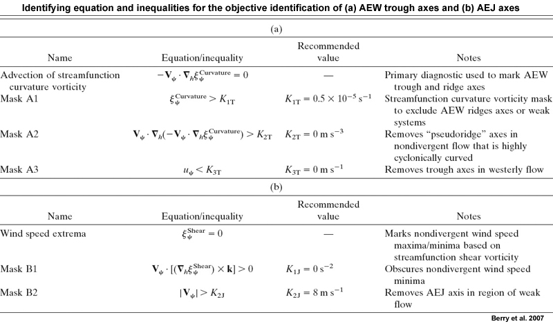
Click above image for a larger view.
http://www.atmos.albany.edu/student/gareth/diagnostics.html
University of Albany Real-time maps of troughs and jets,
http://www.atmos.albany.edu/student/janiga/web/regional_maps.htm
Brief Biographies
Robert (Bob) Burpee
Dr. Robert Burpee was a research meteorologist who pioneered the incorporation of aircraft data into hurricane forecasting models, improving their accuracy. He also served as director of the National Hurricane Center from 1995 to 1997. Burpee received degrees from Harvard University and the Massachusetts Institute of Technology. He went to Miami in 1967 to work on the first dynamical hurricane prediction model as part of his Ph.D. work. He also studied the tropical easterly waves that give rise to hurricanes, which ultimately became the basis of his dissertation. Starting in 1971, he worked as a researcher and then director (from 1993-1995) of the NOAA Hurricane Research Division on Virginia Key, Florida.
It was his idea to fly aircraft into hurricanes and add that information to computer forecast models, which improved their accuracy by 10-15 percent. In 20 synoptic flow experiments that took place between 1982 and 1986, NOAA flew WP-3D research planes into hurricanes and released dropwindsondes to obtain wind, temperature, and humidity profiles. The success of this experiment led NOAA to buy G-IV jet hurricane hunter aircraft, one of the largest investments NOAA ever made for hurricane forecasting. He was a consummate and ethical scientist devoted to data who also counseled many of his colleagues personally. He was also courageous flying through the eyes of hurricanes more than 260 times. In addition to his work on hurricane forecasting, he also did important early research on the Florida sea breeze that generates daily rainstorms over the Keys and southern Florida. Dr. Burpee died in 2007.
Toby Carlson
Toby Carlson is a Professor Emeritus of Meteorology at Pennsylvania State University. He is known for his pioneering work on African easterly waves and their role in tropical cyclone formation. He also studied Saharan dust transport across Africa and the Atlantic. In addition to tropical meteorology, his work has encompassed soil moisture, plant transpiration, urbanization, and deforestation by satellite and their applications to regional planning. He wrote A course in tropical meteorology with John Lee. He has also written the textbook MidLatitude Weather Systems that explains the behavior and evolution of weather with conventional weather charts and mathematics. Carlson earned B.S. and M.S. degrees at MIT and a Ph.D. at Imperial College, the University of London. He joined the faculty of the Pennsylvania State University in 1974 after spending nine years at the National Hurricane Research Library. He was also a participant in the GATE experiment, a project to understand cumulus convection in the tropical atmosphere and its role in general circulation. He won a distinguished authorship award from NOAA in 1974. He was named a Fellow of the American Meteorological Society (AMS) in 1993.
Robert Houze
Robert (Bob) Houze conducted fundamental research into the structure and properties of tropical mesoscale convective systems. During his lengthy career, he has studied mesoscale meteorology, radar meteorology, tropical meteorology, hurricanes, orographic precipitation processes, cloud dynamics, cloud microphysics, and storm dynamics. Houze earned a B.S. in meteorology from Texas A&M University in 1967 and a Masters (1969) and Ph.D.(1972) from the Massachusetts Institute of Technology. In 1972, he accepted a position at the University of Washington as Assistant Professor and has been a full professor since 1983. In the 1970s, he did pioneering work on tropical convection during the GATE experiment, a project to understand cumulus convection in the tropical atmosphere and its role in general circulation. He served on the international science team for the Tropical Rainfall Measuring Mission Satellite (TRMM) and participated in its field program in Kwajalein Atoll. He also participated in the Hurricane Rainband and Intensity Change Experiment (RAINEX), in which he directed aircraft into Hurricanes Katrina, Ophelia, and Rita, and he is the author of the textbook, Cloud Dynamics. In 1982 he won the American Meteorological Societys Clarence Leroy Meisinger Award and was named a Fellow in 1993. In 2006, he won the AMS Carl-Gustaf Rossby Research Medal, its highest prize, for fundamental and enduring contributions towards the understanding of the broad spectrum of precipitation systems, their interactions with larger scale circulations, and for his leadership of field programs.
Richard Johnson
Prof. Richard (Dick) Johnson is a professor and former Head of the Department of Atmospheric Science at Colorado State University. His work has centered on the planetary boundary layer and convection: convective weather, monsoon convection, extreme precipitation, and the Western Pacific, Asian, and North American monsoons. He earned a B.S. in physics in 1967 from Oregon State University, followed by an M.S. in geophysical sciences in 1969 from the University of Chicago. In 1975, he completed his Ph.D. in atmospheric science at the University of Washington. He served for two years as a faculty member at the University of Wisconsin before joining Colorado State in 1980 as an assistant professor. He was named full professor in 1986 and department head in 2007. He has studied tropical convective clouds, their effect on tropical circulations, and their interaction with the ocean surface in the Pacific Ocean, South China Sea, and Indian Ocean in detail. He has also studied the East Asian Monsoon and how convection over the South China Sea affects its onset. He is a fellow of the AMS and of the Cooperative Institute for Research in the Atmosphere (CIRA).
T.N. Krishnamurti
Tiruvalum N. Krishnamurti, Professor of Meteorology at Florida State University, conducted important early work in monsoon meteorology, hurricanes, and numerical weather prediction. Within these fields, he has particularly contributed to high-resolution forecasting of hurricanes, forecasting monsoons, and tropical atmosphere variability. Krishnamurti earned a bachelors degree in physics at Delhi University in India and an M.A. in meteorology from Andhra University in Visakhapatnam, India. He traveled to the United States for his Ph.D. in meteorology which he earned from the University of Chicago in 1959. There, he worked with Professor Herbert Riehl and became interested in hurricanes, becoming among the first to fly into the towering clouds out of West Palm Beach and Guam. After earning his Ph.D., he worked at the University of California-Los Angeles for five years before accepting a professorship at Florida State. He helped develop a forecasting method called Superensemble for predicting hurricanes, droughts, and floods, and he has contributed to NASAs Tropical Rainfall Measuring Mission and Laser Atmospheric Wind Sounder. He has won both the International Meteorological Organization Prize from the World Meteorological Organization and the AMS Carl Gustav-Rossby Research Medal, its highest honor, for fundamental contributions to the understanding of the structure and evolution of the tropical atmosphere, especially the monsoons, and for international leadership in the Global Atmospheric Research Programme.
Richard Reed
Dick Reed, was a meteorologist at the University of Washington who on a hunch discovered the Quasi-Biennal Oscillation, a regular reversal of tropical lower stratospheric winds that has major influences on climate. Reed was born in Braintree, Massachusetts, and though he enjoyed math and science in high school, had no particular inclination to any field. He was persuaded by well-meaning relatives to study accounting at Boston College. Unable to afford his second year without working to earn more tuition, he had dropped out of school to work when the Japanese attacked Pearl Harbor. He enlisted in the Navy, and intrigued by the choice of aerology as a specialty by a vague interest in weather, he was assigned to work in that field. After absorbing his first textbook in a single day and night, he was hooked. The Navy sent him to Dartmouth and the California Institute of Technology to further his studies, which completed his bachelors degree. Following the war he earned an Sc.D. in meteorology at MIT in 1949. In 1954, he accepted a position as Assistant Professor in the Department of Meteorology and Climatology at the University of Washington, where he remained the rest of his life. His teaching and research spanned virtually all of meteorology thanks to a deep desire to understand the atmospheres workings. He also fostered pioneering scientific contact with Russia and China during the height of the Cold War. In addition to many other fellowships and awards, Reed won the prestigious AMS Carl-Gustaf Rossby Research Medal in 1989 and was named a member of the National Academy of Sciences. Dr. Reed died in 2008.
links of interest
http://maxmayfieldshurricaneblog.wordpress.com/2007/08/01/tribute-to-dr-robert-bob-burpee/
http://www.met.psu.edu/people/tnc
http://www.atmos.washington.edu/~houze/
http://www.atmos.colostate.edu/faculty/johnson.php
http://www.news.colostate.edu/Release/4283
http://www.nasa.gov/mission_pages/hurricanes/bios/krishnamurti_bio.html
http://eoas.fsu.edu/people/faculty/dr-tn-krishnamurti
http://www.atmos.washington.edu/Reed/
http://www.atmos.washington.edu/Reed/Reed_uweek_org_Vol25_No16_2008.pdf
http://www.atmos.washington.edu/Reed/Reed_Obit_Seattle_Times.pdf