Table of Contents
- 6.0 Overview
- 6.1 Introduction
- 6.2 The Surface-atmosphere Interface
- 6.3 The Atmospheric Boundary Layer
- 6.4 Vertical Transport in Deep Convection
- 6.5 Synthesis: From the Surface to the Tropopause
- Focus 1: Modeling the Tropical Boundary Layer
- Operational Focus
- Summary
- Questions for Review
- Brief Biographies
- References
6.0 Overview
This chapter examines vertical transport of heat, moisture, momentum, trace gases, and aerosols, including the role of tropical deep convection and turbulence. Diurnal and seasonal variations in surface fluxes and boundary layer depth are examined. The boundary layer is compared over the ocean, humid, and dry tropics, including its role in dispersing chemicals and aerosols. Boundary layer clouds are examined in terms of their connection to sub-cloud layer properties. Comparisons are made between heat and moisture transport under a variety of convective modes such as mesoscale convective systems and shallow convection. The trade wind inversion, its maintenance, and east-west structure are presented. The final sections focus on how the tropical sub-cloud layer, clouds, and transport processes are represented in numerical models.
Print Version
The print version provides a single printable page with all required content.
Multimedia Version
The multimedia version provides structured page navigation.
Focus Areas
Quiz and Survey
Take a quiz and email your results to your instructor.
After completing this chapter, please submit a User Survey.
6.0 Overview »
Learning Objectives
At the end of this chapter, learners should be able to do the following:
- Explain the importance of vertical transport in the global energy cycle, general circulation, weather, and climate
- Describe how buoyancy and vertical wind shear contribute to vertical transport
- Describe the basic structure of the tropical troposphere in terms of temperature and humidity
- Describe the role of turbulence and turbulent eddies in surface-to-air transport
- Describe the time scales of vertical motion through different layers in the troposphere
- Describe the structure of the atmosphere boundary layer (ABL) in terms of temperature, moisture, and wind speed
- Describe the role of the ABL in vertical transport
- Understand the basics of how the tropical ABL is represented in numerical models
- Understand the importance of the surface layer to society, weather, and climate
- Recall at least three important surface-to-atmosphere interface processes for land and ocean, respectively
- Describe basic fluxes of the surface energy balance
- Describe the typical diurnal cycle of the surface fluxes
- Identify surface properties based on the partitioning of surface energy components
- Define the Bowen ratio and explain how it is related to climate
- Explain the impacts of vegetation removal on vertical transport and climate
- Understand the importance of the mixed layer in meteorology and climate
- Compare and contrast the convective and stable boundary layers, including their evolution during the diurnal cycle and impact on vertical transport
- Describe the development of the nocturnal low-level jet
- Compare and contrast properties of the mixed layer over ocean and land
- Compare and contrast the mixed layer in the dry and humid tropics
- Describe the transport of energy and momentum fluxes in the mixed layer
- Describe the mechanisms responsible for the formation of the trade wind inversion (TWI)
- Recall and explain the geographic variations in mean TWI structure and its relationship with the tropical marine cloud distribution
- For boundary layer clouds, recall difference in organization and structure based on sub-cloud properties and distance from shore
- Describe the processes that contribute to the growth of tropical cumulus
- Compare and contrast vertical transport in shallow cumulus, deep convection, and mesoscale stratiform clouds
- Understand that in the tropics, most surface to tropopause transport occurs in mesoscale and synoptic systems
- Describe how trace gases and aerosols are transported by tropical clouds
- Compare and contrast the disturbed and undisturbed structure of the cloud and mixed layers
- Define cumulus parameterization and the rationale for its use in meteorology
- Understand the basics of how the tropical sub-cloud and cloud layers are represented in numerical models
6.1 Introduction
6.1 Introduction »
6.1.1 Why Study Vertical Transport?
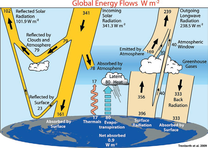
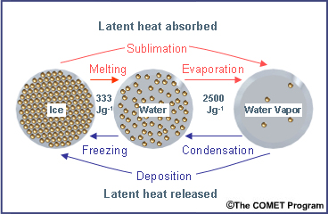
Heat energy input, transfer, and exchange drive the physical cycles of the earth system. Solar radiation is absorbed by the surface then energy is transferred from the surface to the troposphere by latent heat, longwave radiation, and sensible heat (Fig. 1.3). In a very basic sense, vertical transport occurs because surface energy warms the troposphere (heat convergence) while the outgoing longwave radiation cools it (heat divergence). Latent heat (Fig. 5.2), energy stored in water vapor and released into the atmosphere with condensation, is the primary means of surface-to-atmosphere energy transport in the annual global energy budget (Fig. 1.11). Sensible heat flux from the surface, which directly warms the atmosphere, while small in the annual global heat budget, is a significant energy source during the daytime over land.
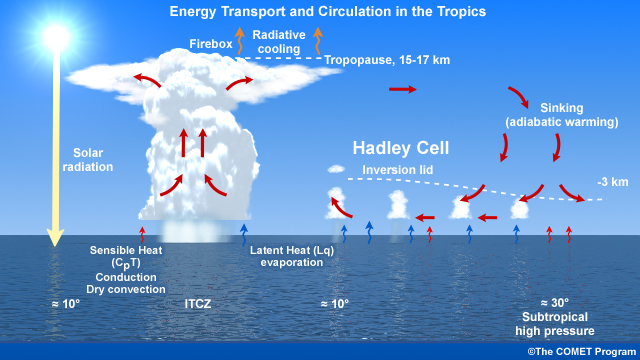
On the global scale, surplus radiative heating in the tropics drives the general circulation of the atmosphere (Chapter 1, Section 1.2Chapter 1, Section 1.2). About half of the energy transported from the ocean to the atmosphere is from tropical oceans. The vast tropical oceans absorb solar radiation leading to high sea surface temperatures (SST). High SST warms and moistens the air above, through sensible heat transport and latent heat transport, leading to instability, rising motion, release of latent heat in deep convection, and transfer of energy and moisture to the atmosphere. The upward motion in deep convection forms part of the Hadley circulation, which has various energy sources and sinks (Fig. 6.1). Furthermore, while the meridional distribution of incoming solar radiation is symmetric, circulations across the tropics are driven by the spatial distribution of vertically integrated net heating across the tropics, e.g., large-scale heating maxima over continents and warm ocean basins leading to the Walker Circulation (Section 3.4Section 3.4). Additionally, the transport of momentum by the Hadley Cells helps to maintain the global angular momentum balance (Fig. 1.28).
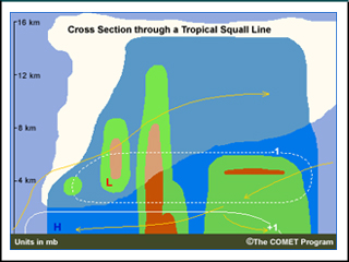
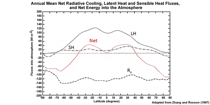
At very large space and time scales, the tropics can be considered to be in radiative-convective equilibrium, where the radiative cooling in the atmosphere is balanced by moist convective heating. The mean temperature profile that results from that equilibrium assumption closely matches the observed mean. However, at local scales such equilibrium does not occur because of atmospheric circulations. Within the troposphere, the latent heat needed to balance the energy lost to radiative cooling in the tropics occurs mainly within tall, rain producing cumulus cores,1 which occupy only small areas of the tropics (Fig. 6.2). Shallow cumuli, which occupy large areas of the tropical oceans2 (Fig. 6.2), also contribute to latent heat transport and radiative cooling.

The latent heat released within deep precipitating cumulus, and their associated strong updrafts and downdrafts that can occupy a deep layer of the troposphere, strongly affect the large-scale dynamics and energetics in the tropics (Section 7.2.2.7Section 7.2.2.7). Latent heat release is critical to the maintenance of organized deep convective systems such as tropical cyclones and mesoscale convective systems. Additionally, cumulus clouds contribute to the global angular momentum budget3 and thereby affect the global circulation. Cumulus convection, described in Chapter 5Chapter 5, is the most important mechanism for the transport of heat, moisture, chemicals/aerosols, and momentum from the local surface to the troposphere as well as through the Hadley circulation (Fig. 6.1). The effects of deep convection on the large-scale are manifested on the order of an hour to several days.
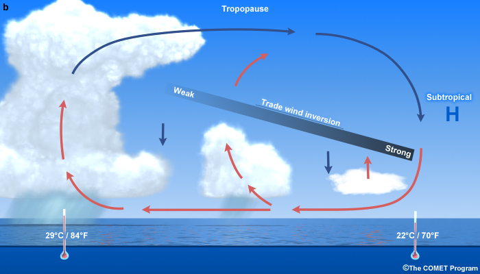
Shallow cumulus and stratocumulus clouds are also important to the large-scale motion and global energy budgets. Large areas of stratocumulus in the eastern tropical and subtropical Pacific and Atlantic Oceans reflect solar radiation, thereby modulating the global radiation budget and climate. Knowledge of the tropical marine boundary layer structure, mixing processes, and transport of chemical helps us to understand marine aerosol concentrations, which affect the radiation budget and air quality. Shallow cumulus also help to maintain the trade wind inversion, by processes described in Section 6.3.7Section 6.3.7. Because of their large spatial extent and persistence in the tropics and subtropics, stratocumulus decks have an impact over long time scales.
While their importance is recognized, convective cloud systems and their internal processes are not easily captured by observation networks and numerical weather and climate prediction model grids. Modeling of individual clouds and their impact in numerical weather prediction (NWP) and climate models is prohibitively complex and too computationally intensive to be achieved in the foreseeable future. In order to quantify cumulus effects on regional and global scales, it is necessary to relate the sub-grid scale cumulus processes to measurable large-scale variables; a process called cumulus parameterization. The parameterization of sub-grid processes also includes the vertical transport of heat, moisture, mass, and momentum. Successful parameterization can only be realized if the processes are (i) identified; (ii) quantitatively related to the resolved model scale of motion, based on intensive field observations that establish an adequate understanding of the physics and dynamics; and (iii) formulated to allow their frequency, intensity, and location to be expressed by the resolved scales.4 The grid scale averages for the transport of heat, moisture, mass, and momentum need to be quantified and verified by observations. In this chapter, we present many examples of observed transport variables and processes.
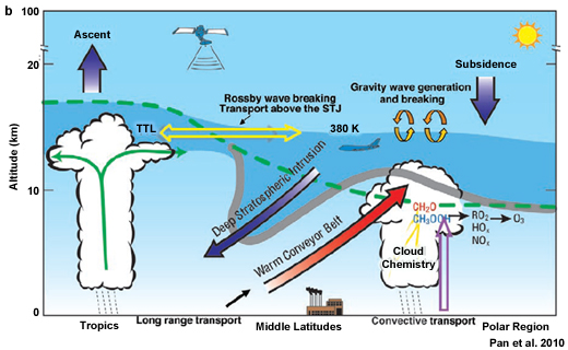
We also need to monitor the movement of gases and aerosols in the atmosphere. This entails understanding (i) properties of the atmospheric boundary layer, a major determinant of near surface air pollution dispersal, and (ii) tropical deep convection, which is the primary conduit for distributing chemical compounds from the surface to the stratosphere, through the tropical tropopause layer (Section 3.2.4.1Section 3.2.4.1). Of particular interest are short-lived chemicals involved in production of ozone and other species of importance to air-quality and radiation budgets, where convective transport processes are vital to their distribution.
In short, vertical transport is critical to understanding atmosphere-ocean interactions; formulating and evaluating NWP and climate models; partitioning global energy and water cycle into oceanic and atmospheric components; and atmospheric chemistry. Before delving further into the processes mentioned above, we will first review the basic vertical structure of the tropical troposphere.
6.1 Introduction »
6.1.2 Vertical Structure and Timescales
6.1 Introduction »
6.1.2 Vertical Structure and Timescales »
6.1.2.1 Mean Vertical Structure
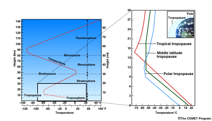
What goes up must come down aptly describes the troposphere, which is a deep layer where upward motion is capped by the tropopause and the stable stratosphere. These basic layers characterize the mean sounding: the atmospheric boundary layer (ABL), the free atmosphere, and the tropopause. The tropopause has its highest global mean in the tropics residing between 15-18 km AGL.
- The ABL, also known as the planetary boundary layer (PBL), is the lowest layer of the troposphere. The ABL is in contact with the surface and experiences frictional effects. Heat, moisture, momentum, aerosols, and gases are exchanged between the free atmosphere and the surface through the ABL. The boundary layer is marked by small-scale turbulent motion and a rapid response to changes in the surface conditions. The boundary layer depth varies from 10s of meters over tropical oceans to several km over hot, dry continents but the typical height is about 1 km. Note that a well-defined boundary layer is not always present. A gradient level is defined for synoptic analysis as the level where friction effects are negligible; around 1 km—a typical ABL height.
- The free atmosphere is unaffected by surface friction. It occupies most of the tropical troposphere and is marked by mostly large-scale subsidence, with upward motion in intermittent deep cumulus and cumulonimbus. Its motions and associated processes have a broad range of time and spatial scales in this layer (Fig. 3.1.4).
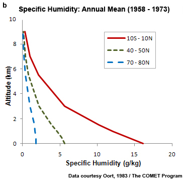
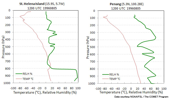
The vertical distribution of temperature and moisture differentiates the tropics from higher latitudes (Fig. 1.16, Fig. 1.19b) and among environments in the tropics (e.g., Fig. 1.20). The free tropical troposphere is often separated from the boundary layer by a temperature inversion, which is stronger with distance from the equator and associated with the descending branch of the Hadley circulation. Mean soundings over various tropical ocean basins generally show high relative humidity in the boundary layer with an approximately linear decrease to a minimum near the tropopause (Fig. 5.20), but some differences are noticeable in the low-middle troposphere. A mean tropical sounding based on observations from the Caribbean (Fig. 5.20a), commonly used as input to idealized tropical numerical models, is relatively dry in the low-middle troposphere (Section 5.2.4Section 5.2.4). The vertical structure in the Caribbean is influenced by maritime tropical air mass, as is common in other tropical basins; the dry, low-middle troposphere Saharan Air Layer, which emanates from northern Africa; and a dry, midlatitude air mass that intrudes periodically into the tropics with midlatitude cyclones and troughs. The West Pacific is generally warmer and moister than other tropical basins but is also affected by dry midlatitude air masses. The vertical structure varies in a given region or time or in the presence of convection, when fluxes of heat, moisture, and momentum, can differ greatly from the mean and fair weather environment.
6.1 Introduction »
6.1.2 Vertical Structure and Timescales »
6.1.2.2 Time Scales of Vertical Overturning
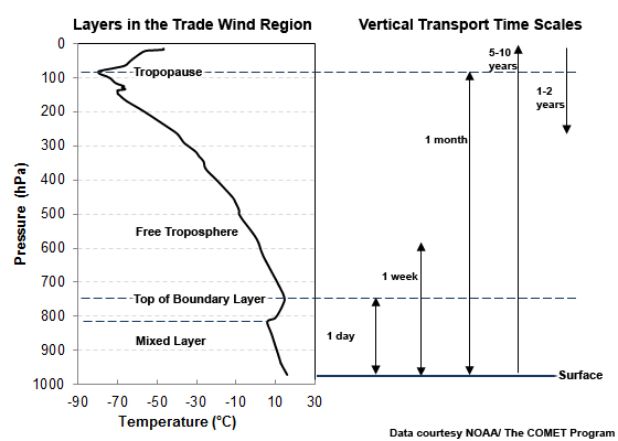
Mixing between the surface and the top of the ABL occurs during 1 hour to a day while overturning of the free troposphere is on the order of a week to one month (Fig. 6.3). Convective overturning takes 4-5 months at the base of the tropical tropopause layer (TTL, Fig. 3.18) and 1-2 years at the tropopause. The transport of air through the strong inversion above the tropopause takes 5-10 years and about 1-2 years for downward transport. Transport from the troposphere to the stratosphere occurs mainly in the tropics, while the reverse transport is mostly in the midlatitudes (Section 3.2.4.1Section 3.2.4.1). Within deep convection, BL air can reach the upper troposphere in mere hours.
The interactions between the surface and the upper troposphere occur through a continuum of scales such as the Walker Circulation and its interannual oscillations, the MJO on intraseasonal time scales, through thunderstorms on diurnal time scales, and the mixed layer in about an hour. Those are just a few examples of how knowledge of vertical transport helps us to understand the major modes of tropical variability and the means by which energy and momentum move from the surface to the top of the troposphere. Given the principal role of air in motion to energy transfer from the surface (Section 6.1.1Section 6.1.1), we will next review mechanisms that move air vertically.
6.1 Introduction »
6.1.3 Vertical Motion Mechanisms
6.1 Introduction »
6.1.3 Vertical Motion Mechanisms »
6.1.3.1 Buoyancy and Static Stability
Buoyancy (Box 5-3Box 5-3), the net vertical force exerted on an object in a fluid, is proportional to the difference in density between an object and the fluid in which it is immersed. If an object is lighter, it will accelerate upwards, if heavier, it will sink. Whether a displaced air parcel will rise or sink, due to buoyancy, depends on whether conditions are stable, neutral, or unstable.

With the assumption that air parcels undergo adiabatic warming and cooling, dry air parcels will cool at the dry adiabatic lapse rate (~9.8 °C/km), while saturated air parcels cool at a slower rate because of latent heat release with condensation. In what is called the parcel method of stability assessment, the environmental and parcel temperatures are compared since warmer (less dense) air will rise relative to cooler (denser) air:
- Stable: With warmer environment after an initial upward displacement, the parcel will sink
- Unstable: With cooler environment after an initial upward displacement, the parcel will rise
- Neutral: With the same temperature, the parcel will remain neutrally buoyant
- Conditionally unstable: Stable except for rising or sinking parcels that are saturated with water vapor
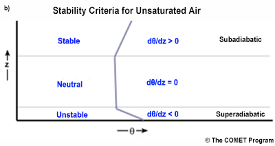
The temperature profiles associated with stable, neutral, and unstable conditions are illustrated in Fig. 6.4a. Stability is also assessed from the vertical gradient of potential temperature, θpotential temperature, θ, where δθ/δz > 0 is stable, δθ/δz = 0 is neutral, and δθ/δz < 0 is unstable (Fig. 6.4b). Stability for moist convection is determined from the vertical gradient of the equivalent potential temperature: δθe/δz > 0 is stable, δθe/δz = 0 is neutral, and δθe/δz < 0 is unstable. The local value of the lapse rate determines local stability, so the atmosphere may have stable and unstable layers. Instability promotes rapid vertical mixing because buoyancy accelerates an initial push on an air parcel.
Mass Continuity
According to the general principles of mass continuity for large-scale motion, horizontal divergence is proportional to a change in vertical motion with height (Section 3.1.1Section 3.1.1). In applying this principle to the tropical atmosphere, near surface horizontal convergence must result in ascent to the tropopause, a stable barrier to further ascent, so air diverges. Correspondingly, sinking motion leads to near surface divergence. As we will see later, large-scale sinking motion in the subtropics is instrumental in establishing the vertical structure and is a major factor in vertical transport processes in the trade wind regime.
6.1 Introduction »
6.1.3 Vertical Motion Mechanisms »
6.1.3.2 Turbulence
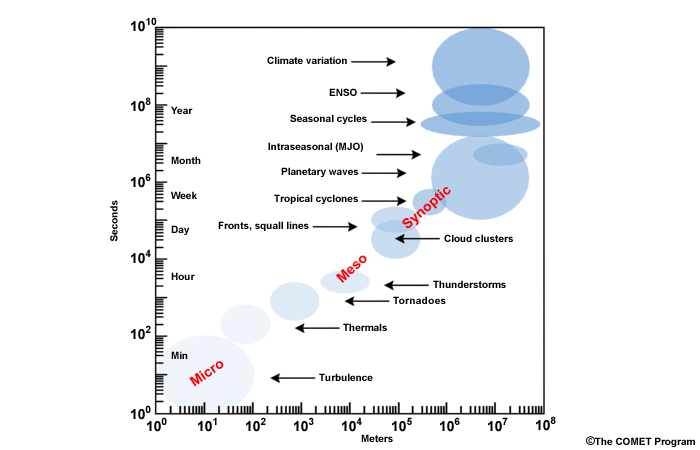
Turbulence refers to irregular fluctuations occurring in fluid motion, which is apparent as swirls, called eddies. Turbulent eddies are microscale (Fig.3.4), having length scales of millimeters to a few kilometers and time scales of seconds to near an hour for the larger eddies.5,6
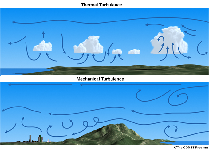
Turbulence is a primary mechanism for vertical motion in the boundary layer where flow is directly influenced by the surface heating and friction. It occurs in the free troposphere because of processes such as wind shear associated with jet streams, updrafts and downdrafts in deep convection, and gravity waves associated with mesoscale convection.7 Turbulent motion, which carries vertical fluxes of momentum, energy, and mass, are generated thermally or mechanically (Fig. 6.5):
- Convective: Generated by buoyancy (Box 5-3Box 5-3) thermals are created when air parcels warmed by the surface accelerated upwards or parcels move downward due to radiative cooling, e.g., at the top of the atmospheric boundary layer
- Mechanical: Generated by vertical wind shear (converts mean wind to turbulent motion)
Small eddies are generated along the edges of large eddies, which lose their energy to the smaller eddies in a process called an energy cascade.
Turbulent and Laminar Flow
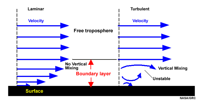
With turbulent flow, there is vertical mixing, while with laminar flow mixing between layers is non-existent or negligible (Fig. 6.6). In experiments with flow in pipes, Reynolds (1894)8 found that the transition from laminar to turbulent flow depends on the ratio of momentum advection to molecular viscosity. Turbulence occurs at a critical Reynolds number, Re, when the flow can no longer sustain the shear.
For the atmosphere, the Richardson number, Ri, used to evaluate whether an atmospheric layer is predominantly turbulent or laminar, is the ratio between the static stability and shear stability. Vertical wind shear can lead to vertical mixing even in a statically stable environment. Using the Brunt-Väisälä or buoyancy frequency, N, as a measure of static stability in a stably-stratified environment, Ri can be expressed as,
 (1)
(1)Here u is horizontal velocity, z is the height, g is the acceleration due to gravity, ρ is the density as a function of height. For small Ri, the shear is enough to overcome the stable stratification; then a shear instability develops. In general,
- Laminar flow becomes turbulent when Ri < 0.25
- Turbulent flow becomes laminar when Ri > 1.0
Sounding data and a finite difference estimate of equation (1) is used to calculate the Richardson number in practice. This form, known as the bulk Richardson number, is:
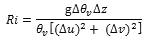 (2)
(2)where Δz is the depth of the layer of interest.
Turbulent Kinetic Energy
The intensity of turbulence is measured in terms of the turbulent kinetic energy (TKE), ē,
 (3)
(3)where u, v, and w are the zonal, meridional, and vertical wind components, respectively. The overbar represents the time average and the prime is the perturbation or eddy contribution. TKE is zero for laminar flow, even though the mean wind components are not necessarily zero.
Vertical motions due to horizontal divergence and convergence in the general circulation are on the order of 0.01 m s-1 while vertical motions due to local buoyancy in deep convection and turbulent processes are more rapid, on the order of 1-10 m s-1. The latter indicates the importance of buoyancy and turbulence in the determination of vertical transport.
Having established the importance of vertical transport in the tropical atmosphere, the typical structure, and the scales and mechanism of vertical overturning, we will now explore in more detail the vertical transport and related processes in the surface-atmosphere interface, the ABL, and the free atmosphere.
6.2 The Surface-atmosphere Interface
The surface interface or contact layer or molecular boundary layer is the boundary between the atmosphere and the ocean or the land. This point of contact is the start of energy exchange between the surface and the atmosphere. In the molecular layer, vertical transfer of
- heat is by conduction,
- moisture is by evaporation/transpiration or condensation, and
- momentum is by viscous processes.
The molecular flux is a product of the diffusivity and the vertical gradient, e.g., the conduction of heat is described by:
 (4)
(4)where v is the molecular thermal diffusivity (˜ 2 × 10⁻⁵ m2 s-1 for air).
The air-to-surface temperature and moisture differences determine the direction of net transfer. For example, when cold air moves over a warm surface, heat is conducted from the surface to the air, resulting in warmer air and cooler surface.
6.2. The Surface-atmosphere Interface »
6.2.1 Air-sea Interface Processes
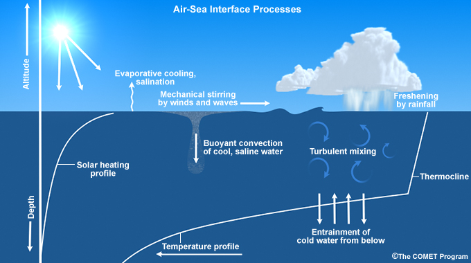
Several interdependent processes at the air-sea interface (Fig. 6.7) are critical to weather and climate and the vertical transport of heat, moisture, and momentum. Evaporation, cooling, and salination contribute to the transport from the ocean to the atmosphere, while rainfall freshens the ocean surface and surface winds generate waves. Coupled with the atmospheric processes are turbulent mixing and entrainment in the upper ocean. Convection is induced in the ocean when the water is cooled and made more saline because of water molecules that evaporated. The thermocline separates the deeper water from the well-mixed upper layer, where the temperature is nearly constant with depth. Variations in the depth of these two layers in the equatorial Pacific are a critical part of the development of El Niño and La Niña conditions.
Chemical transport at the air-sea interface occurs via molecular diffusion and within bubbles and sea spray.9 The latter is produced by wind stress on the ocean surface, most effective at wind speeds > 10 m s-1.10 Sea spray production is most efficient near the crest of breaking or sharply crested waves. Bubbles are generated when precipitation falls on the sea surface and air is entrained within breaking waves.
The SST is observed daily, represents a surface boundary condition for numerical models, and is a critical variable for surface energy budget calculations.
6.2. The Surface-atmosphere Interface »
6.2.2 Land-air Interface Processes

The presence of vegetation adds more complexity to the exchange of energy between the land surface and the atmosphere. With bare soil, the energy exchange is mainly via net radiation, evaporation, and sensible heat; while water flow is through infiltration and runoff. With vegetation (Fig. 6.8), many processes are modified, such as the reflection, IR emission, solar absorption. New processes need to be considered, including: transpiration from leaves; interception of precipitation by foliage; leaf drip; radiation by vegetation; change in the roughness of the surface, which affects the wind shear; and, after recent precipitation, evaporation from wet vegetation.12
A change in land cover, e.g., from forest to grassland will change the albedo, hence the net solar input, the outgoing longwave radiation, evapotranspiration (latent heat), infiltration to the surface, and the roughness height which affects the momentum flux and the heat and moisture fluxes. Generally more arid climates have less vegetation and a greater diurnal temperature range without the modulating influence of water vapor.
The influence and feedbacks of the important land surface-atmosphere interaction processes vary by time scales. Land surface processes are connected to the large-scale dynamics via coupling between the boundary layer, precipitating clouds, and soil moisture and temperature, at diurnal and seasonal time scales.
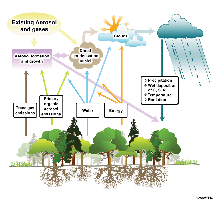
Trace gases and aerosols, which are critical to air quality, radiative heating and scattering, and cloud microphysics, are also transported across the surface-atmosphere interface. Figure 6.9 summarizes important trace gases and aerosol processes over land, including biogenic emissions from the surface to the troposphere, formation and growth of aerosols in the atmosphere, and their return to the surface through precipitation and wet deposition.
6.3 The Atmospheric Boundary Layer
The ABL, which responds rapidly to surface changes, has the following types:
- Convective boundary layer (CBL), a BL that is dominated by buoyant turbulence generation and usually forms in the daytime (Fig. 6.10)
- Stable boundary layer (SBL), which forms at nighttime or when warm air moves over a colder surface
- Residual layer (RL), which may occur during the morning or evening when the previous CBL is disconnected from the surface by the SBL.
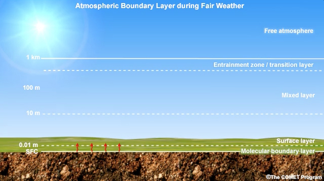
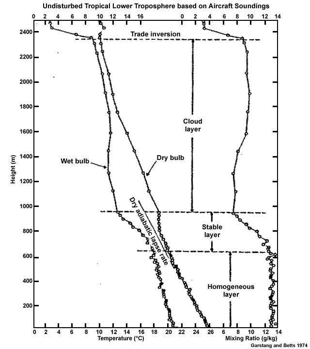
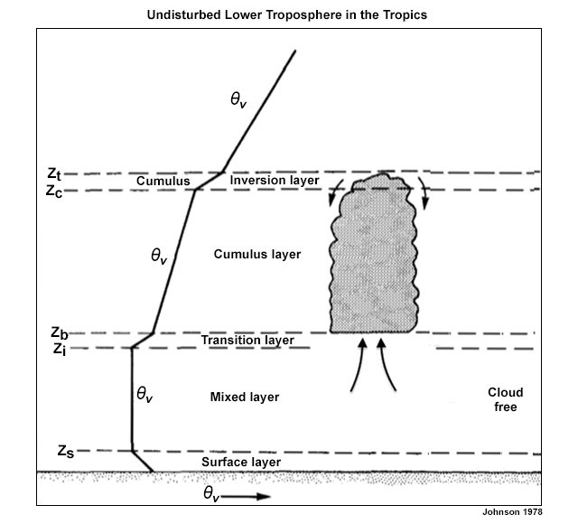
The ABL can be divided into smaller layers based on characteristic thermodynamic and dynamic processes, as illustrated for the undisturbed trade wind conditions in Fig. 6.11. We will examine vertical transport processes in these layers in the next sections.

- The Surface layer, whose base is the contact layer, surface interface, or molecular boundary layer, is the lowest and most shallow part of the ABL (super-adiabatic lapse rate in Fig. 6.11).
- The Mixed or sub-cloud layer, which occupies most of the CBL during daytime over land. It has an adiabatic lapse rate and nearly constant specific humidity, potential temperature, and momentum. It is the homogeneous layer in Fig. 6.11.
- The Transition layer or entrainment zone, which is often capped by an inversion, is where shallow clouds form if the lifting condensation level is reached. Air parcels from the free atmosphere can enter the ABL via turbulent mixing in the entrainment zone. The capping inversion can be eroded with cooling or moistening by turbulent eddy exchange or by large-scale lifting. The removal of the inversion cap can result in rapidly- developing deep convection when the boundary layer is sufficiently unstable.
- The Cloud layer, which extends from the top of the transition layer to the base of the trade wind inversion over tropical oceans.
- The Trade Wind Inversion (TWI) extends above the cloud layer and caps the ABL. Temperature increases rapidly, while moisture decreases. For example, see the temperature and humidity profiles for St. Helena Island (left panel of Fig. 1.20). The TWI will be discussed in detail in Section 6.3.7.
6.3 The Atmospheric Boundary Layer »
6.3.1 Surface Layer
Understanding atmospheric processes in the surface layer is vital because it is where we live and where climate is defined. It is also, typically, where the most dramatic vertical change in temperature and wind velocity occurs. The surface layer depth is about 10% of the depth of a well-developed convective boundary layer (CBL) during daytime or stable boundary layer (SBL) at night.5 The surface layer is marked by strong gradients in humidity, wind speed, and is nearly adiabatic over the tropical ocean and super-adiabatic over land (absolutely instability, where the temperature decrease with height exceeds the dry adiabatic lapse rate).
6.3 The Atmospheric Boundary Layer »
6.3.1 Surface Layer »
6.3.1.1 Surface Energy Balance and Impact on Vertical Transport
The surface energy budget balances the net radiation against the sensible heat, latent heat, storage, and advection:
where Rn is the net radiation at the surface; SH is sensible heat, LH is latent heat, Δf is the horizontal flux or advection; and G is the heat transferred in and out of storage in subsurface layers. The budget does not include negligible contributors such as the conversion of kinetic energy in wind and waves to thermal energy or heat transfer by precipitation.
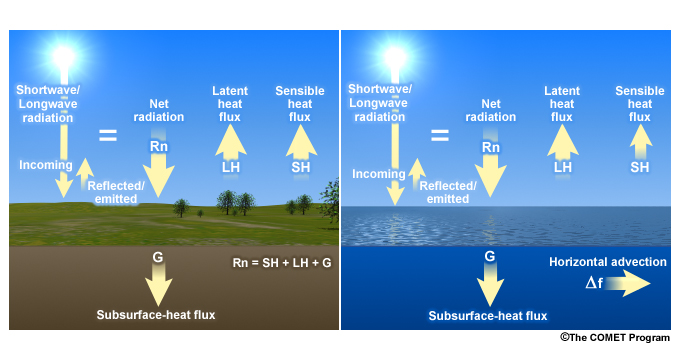
Under steady state conditions, such as for the annual averages or for a day over land, vertical transport of heat at the surface is mainly by radiation, latent heat, and sensible heat (Fig. 6.12). Horizontal transport is significant in the ocean but negligible for land. So the steady-state surface budget for the mostly oceanic tropics can be approximated by:
Latent heat transfer is the primary energy input from the surface to the atmosphere. Annually, the net surface radiation is balanced mostly by the average latent heat, which peaks near 20° latitude (Fig. 1.11). The average sensible heat is relatively small and varies little by latitude except near the poles where it reverses sign as the atmosphere heats the surface.
Changes in the surface energy budget directly affect the vertical transport and the ABL structure. For example, Fig. 6.13 shows how changes in the soil moisture alter the partitioning of the surface energy budget components (sensible heat, latent heat, and radiation), and the vertical transport by convective turbulence. Similar changes are observed between urban and rural surfaces where additional heating in the urban environment16 generates a higher BL over urban areas.
The amount of vertical transport is dependent on the fluxes at the surface interface, which are sensitive to the profiles of temperature, moisture, and wind speed in the air and subsurface. During the day, heat, moisture, and momentum are transported by convection; during the night by conduction at the surface interface. Rooted in the surface layer are thermals or buoyant eddies that drive the circulation in the mixed layer during the day (Fig. 6.10). The surface layer above the interface is a buffer between the interface and the rest of the ABL during the transition from the nighttime SBL to the daytime mixed layer; turbulence in the surface layer allows quasi-constant transport between the interface and the mixed layer. The transport from day to night is more complex, with an initial merging of the surface interface layer and the shallow SBL layer at the surface at sunset.
Question
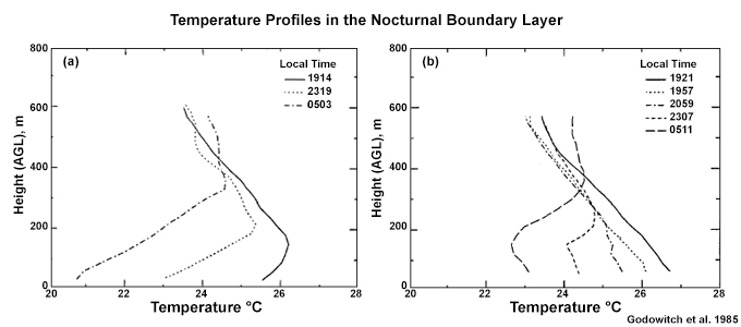
Urban or rural, which of the following temperature plots, (a) or (b), do you think is from each region?
Feedback:
(a) is rural and (b) is urban.17 The rural surface cools relatively quickly during the night leading to an inversion that becomes stronger and thicker through the night. Compare the rural profiles between early nighttime (1914) and early morning (0503). In contrast, the urban area has higher surface temperatures on average and a dry adiabatic lapse rate in the near surface layer even during the nighttime. An elevated inversion forms between near midnight (2307) and the early morning (0511) but it is much weaker than the rural inversion.
Therefore, vertical mixing by convective turbulent continues in the urban residual layer, near the surface, during nighttime. For the rural area, the strong inversion limits mixing to the rest of the boundary layer.
6.3 The Atmospheric Boundary Layer »
6.3.1 Surface Layer »
6.3.1.2 Surface Fluxes of Momentum, Latent Heat, and Sensible Heat
Turbulent Fluxes
The exchange of energy between the surface and the atmosphere is represented by the turbulent or eddy fluxes of sensible heat, latent heat, and momentum. The formulation of the surface flux calculations assumes that transfer occurs mainly in convective cells whose spectrum peaks at wavelengths on the order of one km.18 Vertical fluxes are assumed to be proportional to the local gradient of the mean profiles of temperature, humidity, and momentum.
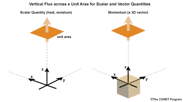
The vertical flux (Fig. 6.14) of any scalar quantity, s, can be calculated as product of that quantity, the vertical velocity, w, and the density of air, ρ. Then the time-averaged vertical flux, Fs, is:
 (7)
(7)Recall from Box 1-1Box 1-1 that variables can be partitioned into their time mean and eddy parts, e.g.,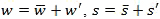 . When wind speed is averaged over half an hour or an hour, the eddy or turbulent parts are the shorter-lived gusts superimposed on the mean wind. This method of quantifying turbulent flows is called Reynolds averaging, which retains non-linear terms that are associated with turbulence.
Recognizing that the eddy flux contributions are much larger than the mean vertical flux near the surface,18,19 we focus on the eddy fluxes. The vertical flux of horizontal momentum at the surface, known as the wind shear stress or Reynolds stress, τ0, represents a drag on air flow at a reference height, z. Reynolds stress at the surface, which deforms an air parcel during turbulent motion, is written as:
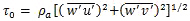 (8)
(8)The surface sensible and latent heat fluxes are then:
 (9)
(9) (10)
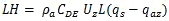
(10)where the overbar indicates a time average, ρa is the air density, q is the specific humidity, L is the latent heat of vaporization; cp is the specific heat at constant pressure, θ is the potential temperature, w is the vertical velocity, and u and v are the zonal and meridional wind components, respectively.
The contributions of the turbulent fluxes to warming and cooling of the atmosphere can be incorporated into the thermodynamic energy equation. The temperature change due to turbulent surface flux would then be written as:
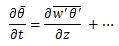 (11)
(11)Wind speed and scaling in the surface layer
- Neutral boundary layer scaling
With a neutral boundary layer (no convection), the vertical gradient of wind speed in the surface layer depends on the height above the surface, density of air, and the surface wind stress, τ0. By rearranging equation (8), a scaling parameter or friction velocity, u*, is defined as:
(12)
Typical values for u* are 0.03 to 0.3 m s-1.
In order to characterize the wind shear for a neutral boundary layer, a dimensionless constant is defined. The von Kármán constant, k, is the same for all neutral boundary layers above any surface and has a value of about 0.4.
The vertical wind shear can then defined as:
(13)
where U is the wind speed, z is the height, and u* is the friction velocity.
- Roughness Length
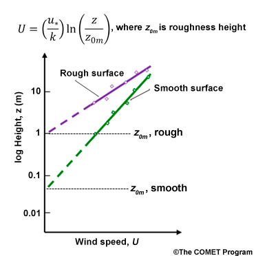
Equation (13) can be integrated to obtain the logarithmic wind profile (e.g., Fig. 6.6) in the neutral surface layer:
(14)
where zom is called the roughness height for momentum.
Fig. 6.15. Logarithmic wind profile, the roughness height is identified where the line crosses zero.The roughness height is the height at which wind speed extrapolates to zero (Fig. 6.15), the zone where transfer is mainly by molecular diffusion. Roughness heights vary from about 1 mm over the average ocean surface to a few cm over grass to more than 1 m over fir forests and cities with tall buildings. Wind profile relationship in (14) is valid for heights that are much higher than the roughness height, not for profiles within the plant canopy or near very rough surfaces.
The scaling parameters for the neutral boundary layer are the friction velocity, u*, and the roughness height, z0m.
- Convective boundary layer scaling
For the CBL, a velocity scale for characterizing turbulent mixing can be defined as:
(15)
where zi is the CBL top, θv0 is a reference temperature,
is the surface virtual temperature flux, g is acceleration due to gravity, and w* is known as the Deardorff velocity scale.20
The scaling parameters for the CBL are w* and the CBL top, zi.
- Eddy circulation time scales
The typical time scales for overturning in the CBL and neutral surface layer are, respectively:
(16)
The time scale for overturning by the biggest eddies in the CBL is on the order of 15 minutes.
Bulk aerodynamic formulae for surface fluxes
Fluxes are not measured routinely but are measured directly during field experiments. For modeling purposes or to create datasets of fluxes, scientists use bulk aerodynamic algorithms that relate the turbulent fluxes to bulk meteorological variable. This is considered to be the most accurate method by which the surface fluxes can be specified in weather and climate models.18,21,22 The turbulent fluxes are assumed to be proportional to the mean wind speed and to the difference between the air and the surface scalar properties. That traditional assumption is based on the Monin-Obukhov similarity theory,23,24,25 which holds that the surface is solid and that surface layer conditions are horizontally homogeneous. Fluxes are assumed to be constant with height and so can be calculated at just one height. This means that turbulent fluxes can be calculated using the mean wind speed at some reference height and empirically-derived transfer coefficients.
The surface momentum flux, τ0, can be written as:
 (17)
(17)CD is the drag coefficient, which depends on the ratio of the roughness height to the near surface reference height, z and ranges from 0.75 × 10⁻³ over smooth surfaces to 2 × 10⁻² over rough surfaces.26 It is a function of height that is estimated by assuming a logarithmic profile that is corrected for the bulk Richardson number. The surface wind speed is usually measured at a standard height of 10 m.
Similarly, the SH and LH can be written in terms of difference between the surface and near surface atmospheric variables at height z.
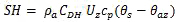 (18)
(18) (19)
(19)where θs and θaz are the surface and near surface air potential temperatures, respectively; qs and qaz are surface and near surface atmospheric specific humidity. CDH and CDE are transfer coefficients for temperature and humidity, respectively. Each is a function of the surface roughness, bulk Richardson number, and the reference height and have typical values of 1 x 10⁻³ to 5 x 10⁻³ (they are dimensionless). The surface temperature and humidity are usually measured at a standard height of 2 m.
QUESTION
Given wind speed of 10 m s-1 on a buoy platform at 10 m and CDH of 3 x 10⁻³, the sensible heat flux would change by _____ W m-2 for each degree of difference between the sea and the air at 10 m. (Choose the best answer.)
Using the bulk aerodynamic formula (19), the sensible heat flux would increase by 30 W m-2 for each one-degree increase in the vertical temperature difference.
6.3 The Atmospheric Boundary Layer »
6.3.1 Surface Layer »
6.3.1.3 Distribution of Surface LH and SH
Geographical and Seasonal Distribution
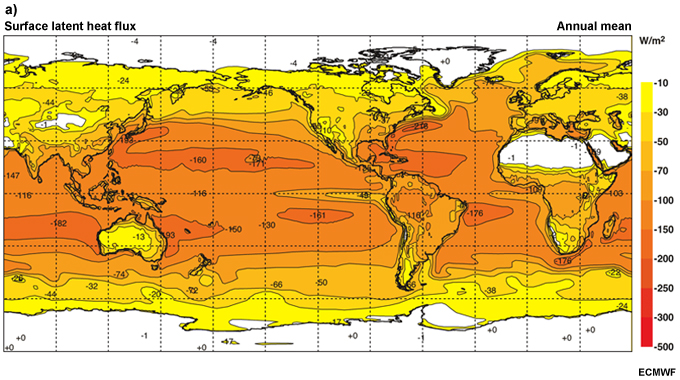
Maxima in annual mean latent heat flux from the surface to the atmosphere occur in the regions of the subtropical ridges: where skies are clear, SSTs are relatively warm, and evaporation is high (Fig. 6.16a). Surface evaporation is also high over the warm ocean currents on the western side of the oceans. The exception is the Southern Indian Ocean, where due to the westerly monsoon winds, a broad maximum occurs over the eastern ocean basin, along the west coast of Australia. Land surface maxima occur over the Amazon, equatorial Africa, and the Maritime Continent, and in tropical rain forests due to the large amounts of evapotranspiration. Minimum surface latent heat flux occurs over subtropical deserts and cool ocean currents.
Mean annual sensible heat flux is maximized over subtropical land areas (Fig. 6.16b), where semi-permanent high pressure leads to clear skies and ample surface heating. As noted in Section 6.3.1.2Section 6.3.1.2, sensible heat flux depends on the air-sea temperature differences and wind speed, thus ocean maxima are found in narrow bands where cool continental air flows over warm ocean currents in the midlatitudes. Gradients are steep in those midlatitude western ocean boundaries but weak in the western half of tropical oceans.
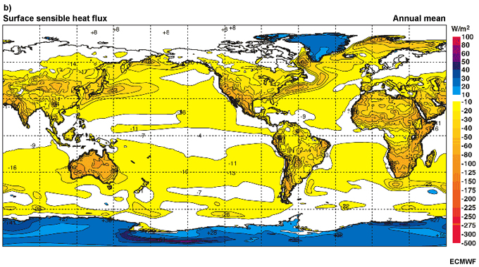
The annual mean latent heat maxima (Fig. 6.16a) reflect the seasonal maxima (Fig. 6.17), which occur over the warm currents during winter. The seasonal maximum in the northern hemisphere (>250 W m-2) is larger than that of the southern hemisphere (>175 W m-2), indicating the critical role of the vertical gradient of moisture in evaporation rates. The difference between the cold continental air masses and warm ocean currents is much larger for the northern hemisphere in winter.
Diurnal Distribution
The diurnal cycle of ocean surface fluxes averaged over the globe is not distinct because SSTs do not vary much on a daily basis; the typical SST diurnal range is 3°C on a clear day with light winds.28 However, year-to-year mean heat fluxes can have differences of up to 10 W m-2 over portions of the tropical oceans.28
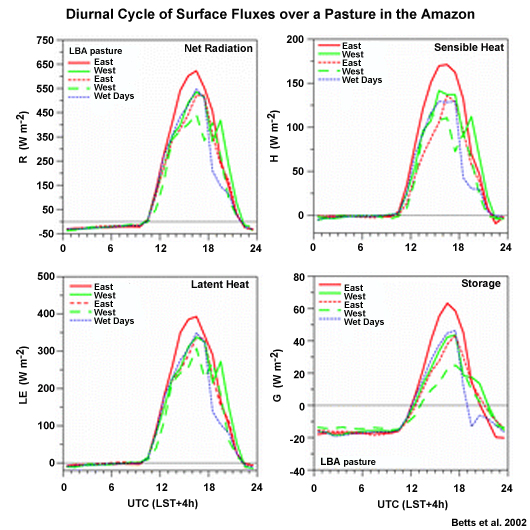
Land surface fluxes have a large diurnal range, generally increase from sunrise to peak around noon and a drop off at sunset and then to remain nearly constant during the night. The diurnal cycle of the surface energy budget components vary across regions and are influenced by transient weather systems. A composite of diurnal cycles over the Amazon (Fig. 6.18) shows the changes in the surface fluxes under varying low-level wind conditions and days when strong rainbands crossed the observation site during the mid-afternoon. The impact of the convective downdrafts during the wet afternoons is clearly seen in all of the graphs, where surface fluxes decreased sharply. The most affected were the sensible heat and storage.
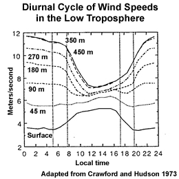
Winds in the boundary layer vary diurnally (Fig. 6.19), which impacts momentum transfers. The most rapid changes in wind speed occur near sunset and after sunrise. During the night, the ABL mixing is reduced and winds weaken in the surface layer and accelerate above the inversion. After sunrise, higher wind speeds begin mixing down to the surface. The result is a mid-afternoon maximum for winds near the surface and a minimum in wind speeds higher in the boundary layer.
QUESTION
Examine the graphs of surface energy budget components during daytime and match the plots to the correct conditions (I, II, III, or IV).
Tab 1
Tab 2
Answer: Tab 1 matches I. Bare soil. Tab 2 matches IV. Wheat field.
For the bare soil surface, most of the surface to air transport is in the form of sensible heat flux with relatively small latent heat flux. For the wheat field, the latent heat flux exceeds the sensible heat because of transpiration and greater evaporation. The schematic diagrams in Fig. 6.13 show the impact of variable wetness on the partitioning of the surface heat budget. Both dry and moist convection are enhanced for the wheat field, which has more roughness than bare soil; so the flux values are closer for the wheat field.
6.3 The Atmospheric Boundary Layer »
6.3.1 Surface Layer »
6.3.1.4 Bowen Ratio
The Bowen ratio,31,32 B, is the ratio of the sensible heat to the latent heat (B=SH/LH). Changes in the surface energy budget, such as caused by changes in vegetation or anomalous precipitation, control the Bowen ratio. The Bowen ratio is highly varied over land, where it is determined by fraction and type of vegetation; soil moisture; temperature (because of the temperature dependence of saturation vapor pressure known as the Clausius-Clapeyron relationship (Section 5.1.2Section 5.1.2), and entrainment of dry air into the boundary layer. Over the desert, most of the surface to air transfer is by the sensible heat, warming a deep, dry BL; while over forested areas, most of the transfer during daytime is by evaporation (latent heat). An increase in the Bowen ratio indicates that an area is becoming more arid (Table 6.1).
| Surface Type | Bowen Ratio |
| Open Tropical Ocean | 0.07 |
| Tropical Rainforest | 0.1-0.3 |
| Daytime over grassland | 0.3 |
| Australia (mostly dry continent) | 2.18 |
| Semi-arid | 2.0-6.0 |
| Desert | >10.0 |
6.3 The Atmospheric Boundary Layer »
6.3.2 Mixed Layer
The mixed layer, which occupies most of the ABL, is responsible for vertical transport between the surface layer and the entrainment zone or transition layer (Fig. 6.11). Mixed layers occur even with weak surface heat fluxes over the equatorial ocean. The mixed layer plays a critical role in the distribution of pollutants. The top of the mixed layer, zi, marks the level to which turbulence has a significant influence.
6.3 The Atmospheric Boundary Layer »
6.3.2 Mixed Layer »
6.3.2.1 Mixed Layer Depth
The structure of the mixed layer varies according to meteorological conditions but it is generally deeper (higher) when both convective and mechanical turbulence are strong, such as:
- above a heated surface,
- over a rough surface,
- when strong winds are present, and
- when the mean vertical motion in the free atmosphere is upward.
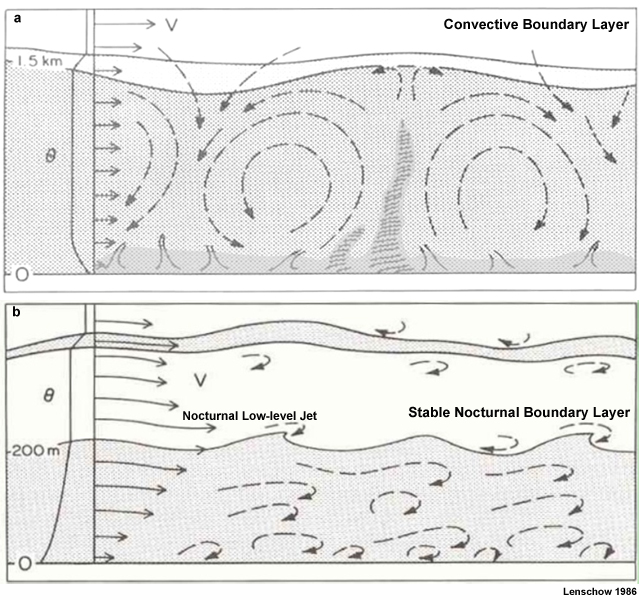
Figure 6.20 illustrates the contrast between the daytime CBL, with vertical motion in thermal circulations and top height at about 1.5 km, and the nocturnal SBL, with predominantly laminar (horizontal) flow and top height at about 200 m.34 During the day, under strong solar heating, the boundary layer is dominated by convective turbulence as the heated surface warms air parcels, which move upward due to buoyancymove upward due to buoyancy. At night, the land surface cools more rapidly than the air, which creates an inversion and a stable boundary layer. With colder, dense air trapped near the surface vertical motion is suppressed and the surface is mechanically de-coupled from the free atmosphere. Any vertical mixing is then due to the wind shear, which can be strong, as a low-level wind maximum or a low-level jet (LLJ) often forms near the top of the nocturnal boundary layer, with weak winds near the surface.
The height or thickness of the convective boundary layer (zi) is a fundamental, controlling length scale for many tropospheric processes such as turbulent mixing, vertical diffusion, transport by convection, and entrainment of clouds and aerosols. It broadly defines the vertical depth of significant influence for turbulent transport from the surface and helps to determine cloud type and cloud coverage, thereby affecting the global radiation budget. The CBL height also determines processes that affect air pollution, including the distribution of aerosols, fog and cloud formation, convective activity, and the assessment of air quality at local and regional scales.35 Model boundary layer parameterization schemes are evaluated by their ability to calculate boundary layer turbulence, which depends on the boundary layer height.36
The CBL height, zi, is defined by the base of the lowest inversion in the absence of clouds; also the top of the mixed layer. However, zi is not routinely or directly observed in meteorological operations. Instead, it is usually estimated from vertical profiles of:
- Temperature (Fig. 6.11a)
- Dew-point temperature (Fig. 6.11a)
- Mixing ratio or specific humidity, q, conserved for adiabatic processes, (Fig. 6.11b, 6.21)
- Potential temperature (θ), conserved for adiabatic processes,

- Virtual Potential Temperature (θv, Fig. 6.11b) - for unsaturated air, θv is given by θv = θ(1 + 0.61q).
- Dry static energy (s), the equivalent of the potential temperature when altitude is used as the vertical coordinate; s = cpT + gz (Section 5.2.3Section 5.2.3)
- Refractivity - derived from Global Positioning System (GPS) radio occultation(GPS) radio occultation, assumes that the ABL is moister, denser, and more refractive than the free troposphere.37
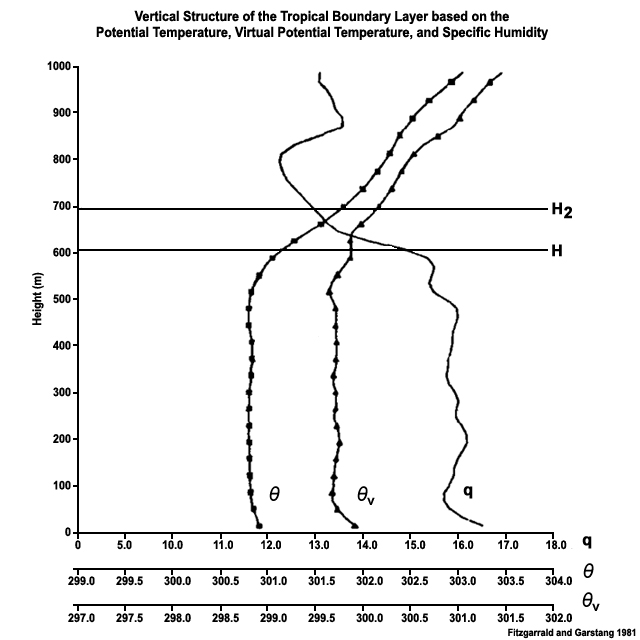
A common marker for zi is the inflection point in the region of maximum vertical gradients of θ, θv, and q;39,40 shown for a tropical marine boundary layer in Fig. 6.21.41 Mixed layer potential temperature, momentum, and moisture vary little with height compared with large gradients in the surface layer (below) and the entrainment zone (above). The convective BL top is most well defined as the base of a capping inversion, which impedes the rising thermals (shown schematically in Fig. 6.20a). The ABL height for neutral and stable boundary layers is more uncertain. For the SBL, the top is where turbulence from the surface nearly ceases, but is more difficult to identify because the turbulence is weaker and the layer more shallow (Fig. 6.20b), and turbulence is not routinely measured. One objective technique to identify zi is denoting it as the height at which an air parcel that is rising adiabatically from the surface becomes neutrally buoyant.5,42 Lidars are also used to measure the CBL height; measurements determined by radiosonde and lidar can differ by about 200 m.42
Merged Profiles Improve Definition of Planetary Boundary Layer Height,
http://asr.science.energy.gov/news/data-announcements/post/4728
https://www.arm.gov/data/pi/65
6.3 The Atmospheric Boundary Layer »
6.3.2 Mixed Layer »
6.3.2.2 Effect of Synoptic Highs and Lows
The BL is shallower in centers of high pressure, because of subsidence and divergence in the lower troposphere (Fig. 1.18). The depth increases with distance from the high center as subsidence weakens. In regions of low pressure, air in the boundary layer rises to form clouds in the free atmosphere. The cloud base is then considered to be the top of the CBL, which is not easy to discern from soundings.
6.3 The Atmospheric Boundary Layer »
6.3.2 Mixed Layer »
6.3.2.3 Mixed Layer in Disturbed and Undisturbed Conditions
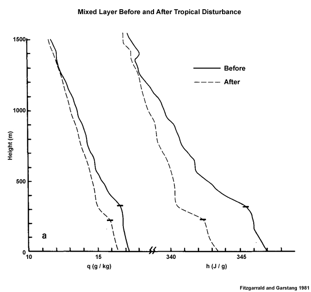
The undisturbed mixed layer has the structure described in Section 6.3.2.1Section 6.3.2.1 and shown in Fig. 6.21. During disturbed periods, the mixed layer becomes cooler and shallower. Fig. 6.22 shows the effect of a tropical disturbance over the tropical Atlantic, which is to lower the specific humidity, moist static energy, and mixed layer height. The scale of change in the sub-cloud layer properties depends on the size and intensity of the convective system as well as the time history of the interactions between the convection and the mixed layer. It is suggested that the sub-cloud layer in the equatorial trough may be modified by deep convection about one-third of the time.43
6.3 The Atmospheric Boundary Layer »
6.3.3 Marine and Land Boundary Layers
Since the growth of the mixed layer depends on surface fluxes and stability, it is higher over land, where fluxes and instability are greater, than over the ocean. Dry convective boundary layers are dominant over land, while stratocumulus-topped boundary layers are more prevalent over ocean. Typical BL height over the tropical ocean is 424 m (standard deviation = 160 m),41 while height over land can be ≥ 1200 m.
The marine boundary layer depth varies slowly because SSTs evolve slowly due to the larger specific heat of the ocean. The mean evaporative flux in the mixed layer over ocean is a little over 1/3 of the daytime flux over tropical forests,44 which change dramatically during daytime. However, ocean fluxes persist through 24 hours and dominate at long time scales because the tropics are mostly ocean. Differences between the BL over the ocean and over land (Table 6.2) are driven by the differences in the air-sea and air-land interface characteristics. The main distinctive marine attributes are:
- Less friction, which means that for the same pressure gradient and Coriolis force, ocean winds will be closer to geostrophic (less cross-isobaric flow) and faster than over land (an exception might be during high seas)
- SSTs are relatively unchanging at diurnal scales, compared with land surface temperatures changes that affect the lapse rate and hence stability at short time scales
- Momentum transfer into wave energy and wave dynamics
| Marine BL | Continental BL |
| Little diurnal variability | Strong diurnal variability |
| 1-2 km height (500 m over eastern tropical oceans) |
Up to 5 km height over deserts |
| Stratocumulus and trade cumulus topped most common | Dry convective |
| Low roughness length | High roughness length over forest and cities with tall buildings |
| Wave state is important (affects momentum transport) |
Fixed surface shape but important |
| Less friction, less cross-isobaric flow (except maybe in high seas) | Greater friction, more cross-isobaric flow |
| Small Bowen ratio (SH/LH) |
Large Bowen ratio |
Interestingly, double mixed layers were observed over the western Atlantic during the Barbados Oceanographic and Meteorological Experiment (BOMEX),45 the Central Arabian Sea during Indian Ocean Experiment (INDOEX),46,47 and the Bay of Bengal during the Integrated Campaign for Aerosols, gases and Radiation Budget (ICARB).48 One explanation for the double structure is precipitationevaporation processes45 but further study is needed to understand the mechanisms.
6.3 The Atmospheric Boundary Layer »
6.3.4 Diurnal Cycle of the ABL
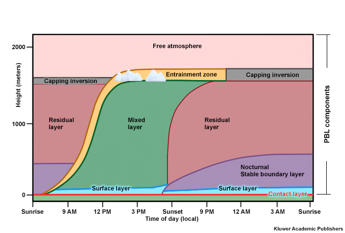
The idealized diurnal cycle of the ABL over land in the tropics, which is similar to the midlatitudes, can be divided into a convective boundary layer (CBL, occupied mostly by the mixed layer), a stable boundary layer, and a residual layer (RL) (Fig. 6.23). A neutral residual layer is defined when parcels are neutrally buoyant for an RL that starts from the ground. The differences between the nighttime and daytime ABL influences many processes including the surface concentration of pollutants, a major societal and public health concern.
6.3 The Atmospheric Boundary Layer »
6.3.4 Diurnal Cycle of the ABL »
6.3.4.1 Diurnal cycle of mixed layer over land and ocean
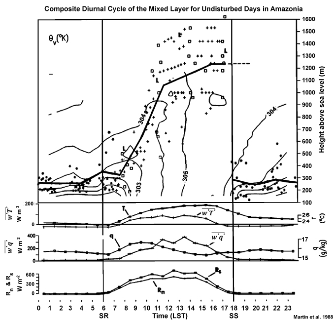
 , temperature Τ, moisture flux,
  , specific humidity q, incoming solar radiation flux Rs, net radiation flux Rn, and rainfall, all measured at the micrometeorological level. The and were measured at the 40-m level; the other parameters were measured at the 45-m level. SR and SS are approximate sunrise and sunset.44
Vertical mixing of the unstable mixed layer over land, produced by solar heating, occurs in less than an hour. The mixed layer depth increases between sunrise and sunset, then active mixing ceases (Fig. 6.24). A residual or fossil mixed layer remains, with no new mixing and the remaining turbulence is negligible as shown by the values of the eddy heat and moisture fluxes (lower panels of Fig. 6.24). The residual layer retains the properties of the daytime mixed layer, with variations only due to radiative cooling or horizontal advection. Surface heating during the next diurnal cycle recouples the surface layer to the mixed layer, which begins its daytime growth anew.
The vertical eddy flux of sensible heat reaches maximum around noon, matching the graph of the net radiation, while the latent heat flux reaches its maximum 1-2 hours later. Although the specific humidity, q, peaks in the morning, the latent heat flux peaks in the afternoon because evaporation rate depends on temperature (Chapter 5, Section 5.1.2Chapter 5, Section 5.1.2).
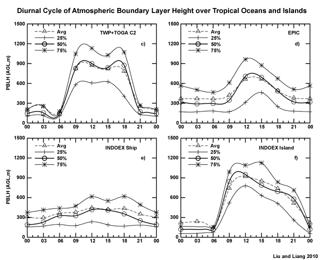
Observations from tropical field campaigns (referenced in Fig. 6.25) found a strong diurnal cycle in the height of the ABL, with a peak of 1500 LST over land and 1200 LST over the ocean (Fig. 6.25). Over tropical oceans, the growth and decay of the mixed layer is more gradual and more symmetric about the maximum.42
Nocturnal Low-Level Jet
The nocturnal low-level jet (NLLJ) is a common feature of the stable nocturnal boundary layer during undisturbed conditions in non-mountainous terrain.49,50,51 The typical nocturnal jet is found between 100-300 m above ground (e.g., Fig. 6.20b), with maximum wind speeds of 10-20 m s-1.52
We are interested in the NLLJ because it can generate shear and turbulence between the jet and the surface, thereby influencing surface-to-atmosphere exchanges at night.53 It can be hundreds of km wide and thousands of km long and acts as a channel for moist, unstable air to fuel nighttime convection (Section 7.2.2.4Section 7.2.2.4), a major vertical transport process. The jet usually reaches its peak speeds near midnight, persists until sunrise, and then decays with the onset of daytime heating as wind speeds become more uniform in the mixed layer.
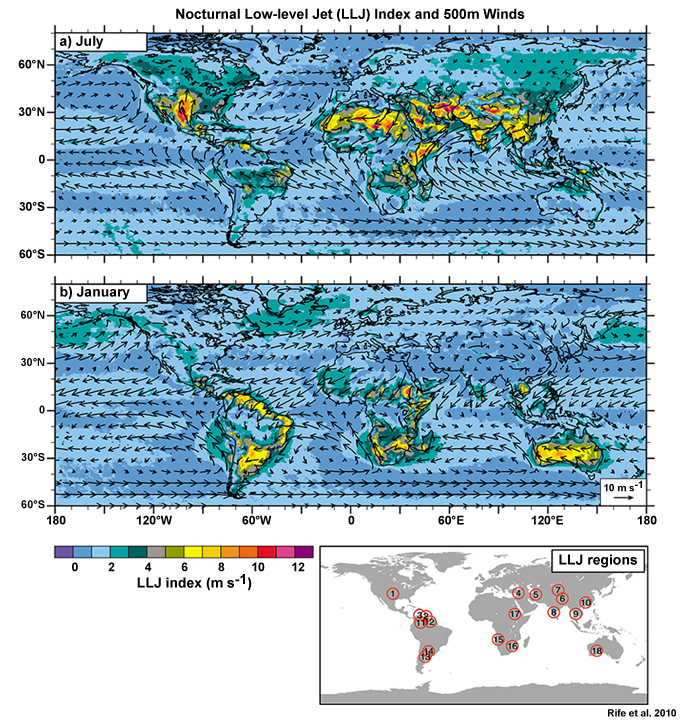
Nocturnal LLJs are found in many areas of the tropics. Figure 6.26 shows recurring NLLJs and an index that identifies their location and peak time of occurrence. Their formation has been attributed to two major mechanisms: diurnally varying friction in the boundary layer49 and diurnal thermal forcing over sloping terrain.50
Diurnally varying friction in the boundary layer
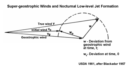
After sunset, the land surface cools rapidly creating a surface inversion and a stably-stratified boundary layer (Fig. 6.20b). According to Blackadar (1957),49 with the assumption of constant pressure gradient force with no friction, the flow above the inversion is governed by Coriolis or inertial oscillations. Thus, flow accelerates in response to the imbalance between the Coriolis and pressure gradient forces, creating a low-level wind maximum or jet at the top of the inversion.
Fig. 6.27. Development of supergeostrophic winds in the low-level jet (after Blackadar 1957)49, where Vg is the geostrophic wind, V0 is the initial wind, and V the true wind. W is the deviation from the geostrophic wind at some time t, W0 the deviation at initial time.55The magnitude of the deviation from the geostrophic wind remains the same but is deflected by the Coriolis force over the course of the night. Wind variations mark out a circle over time (Fig. 6.27) with maximum wind speed at about time, t = π/f hours after sunset, where f is the Coriolis parameter. At each level, the wind vector rotates clockwise with diurnal periodicity in the Northern Hemisphere (counter-clockwise in the Southern Hemisphere). Because of the dependence on the Coriolis effect, this mechanism for the NLLJ formation is more applicable at higher latitudes (usually ≥ 30° latitude) but can sometimes be important at low latitudes, as documented for northern Australia.56
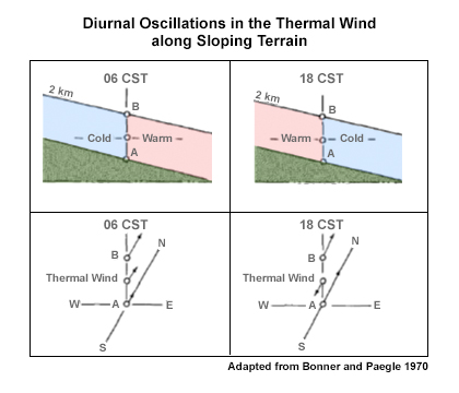
Diurnal thermal forcing over sloping terrain
This theory focuses on the preference for nocturnal LLJs to form over the sloping terrain. Holton (1967) found that a diurnal wind oscillation can be induced in the boundary layer over a sloping surface as a response to a diurnally varying and deep volumetric heating/cooling function.
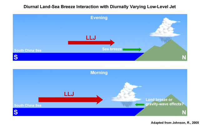
Fig. 6.28. Conceptual representation of oscillations in the thermal wind.57The formation and decay of the nocturnal LLJ is also promoted by the rotation of the thermal wind due to the thermal contrast over the sloping terrain (Fig. 6.28).57 Similar mechanisms are associated with LLJs generated by land-sea thermal contrast in places like the South China Sea (Fig. 7.119). Combining the inertial oscillation theory with the sloping terrain effects has produced more realistic jet phases and structure.58
Other related processes include propagation of gravity waves beneath an inversion and local pressure gradients induced by large bodies of water, such as the Amazon River. Nocturnal LLJs are stronger when skies are clear, which leads to more radiative cooling. In the equatorial rainforests, they tend to be absent during rainy or overcast conditions.
Diurnal cycle in the humid and dry tropics
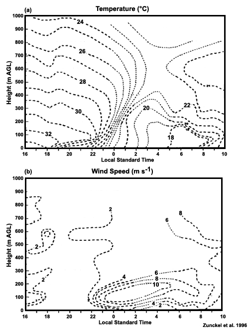
The diurnal changes in the surface temperature, winds, and vertical gradients are very pronounced in the dry, tropical and subtropical savannas (Fig. 6.29). For example, in southern African savannas, diurnal temperatures range from about 40°C during daytime to about 5°C at night.60 In the example shown, coincident with rapid surface cooling is the calming of wind speeds at the surface. By about an hour after sunset an LLJ (> 12 m s-1) forms over the surface inversion at about 200 m above the surface. The LLJ persists until just after sunrise.
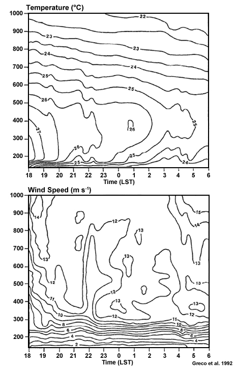
The near-surface conditions within a rain forest with closed canopies are quite different from the evolution over the open tropical and subtropical savannas. Within the forest canopy, wind speed or wind profiles vary little between day and night and the diurnal surface temperature range is only a few degrees (Fig. 6.30). Nevertheless, a nighttime inversion decouples the surface canopy from the rest of the BL. The top of the inversion is about 400 m (twice the height of the arid region in Fig. 6.29). A period of strong low-level winds occur around midnight but compared with the uniform and steady LLJ in the arid tropics, the nocturnal winds over this tropical forest is much more varied in its vertical structure and in time.
6.3 The Atmospheric Boundary Layer »
6.3.4 Diurnal Cycle of the ABL »
6.3.4.2 Seasonal Variations
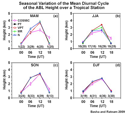
The seasonal range of the ABL height is much smaller than the diurnal range but is still significant. The ABL depth, given its response to surface heating, is generally greatest during summer and lowest during winter. In monsoon regions, the ABL is highest during the pre-monsoon when skies are relatively clear and the surface temperature is highest (see Fig. 1F2.5). With the arrival of monsoon clouds and rains, the ABL is lowered then reaches a minimum during winter. Figure 6.31 shows the effect of the seasonal cycle on the diurnal range of the CBL in southern India, with maximum heights and range during the pre-monsoon (March-May) and minimum during winter. Notice the wider spread in the estimated heights during June-August, indicating the difficulty in defining zi during precipitating convection (Section 6.3.2.1)Section 6.3.2.1).
6.3 The Atmospheric Boundary Layer »
6.3.5 Boundary Layer Clouds
Clouds in the tropical marine boundary layer lie between the mixed layer and the trade wind inversion (Fig. 6.11). The tropical convective boundary layer over the ocean is fairly uniform with cloud-base near 950 hPa. Boundary layer clouds have roots in the mixed/sub-cloud layer, with coherent updrafts observed 200-300 m below cloud base.63 While not as common as fair weather cumulus or stratocumulus, fog is also a boundary layer cloud.
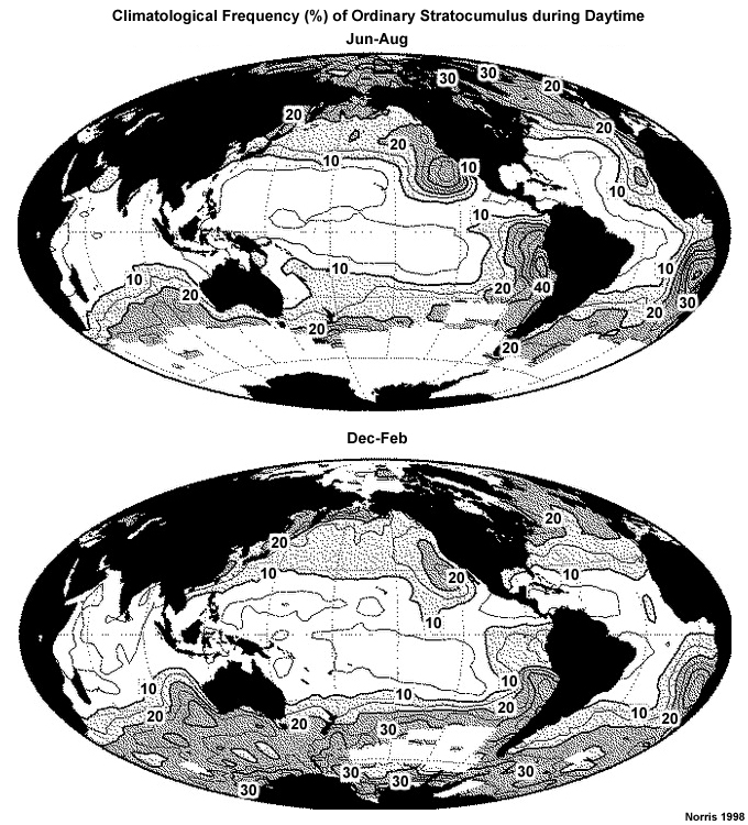
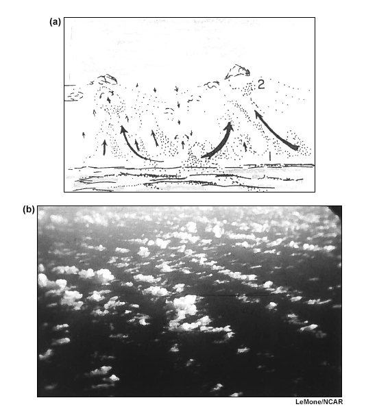
Shallow non-precipitating stratocumulus/cumulus clouds are part of the convective boundary layer that covers most of the tropical oceans outside of the atmospheric convergence zones (Fig. 6.32). Clouds are limited to the boundary layer in regions of subsidence and a strong trade wind inversion.
6.3 The Atmospheric Boundary Layer »
6.3.5 Boundary Layer Clouds »
6.3.5.1 Boundary Layer Cloud Morphology
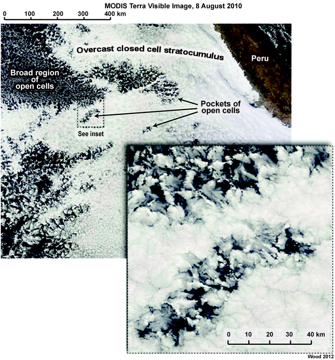
As noted in earlier chapters, tropical convection is most often organized at the mesoscale in deep convection. Shallow convection can be organized into two distinctive forms on the mesoscale: linear and hexagonal; others are simply random. Shallow clouds are usually 1 to 2 km deep, with horizontal length scale of a few to a few tens of kilometers. The hexagonal forms are called mesoscale cellular convection,65 comprising three-dimensional open or closed cells (Fig. 6.33), while the linear form is called a horizontal convective roll, cloud street, or cloud band. The typical width to height aspect ratio of horizontal convective roll is 3:166,67 but can reach 6:1 or more where cold air flows over warm water.68
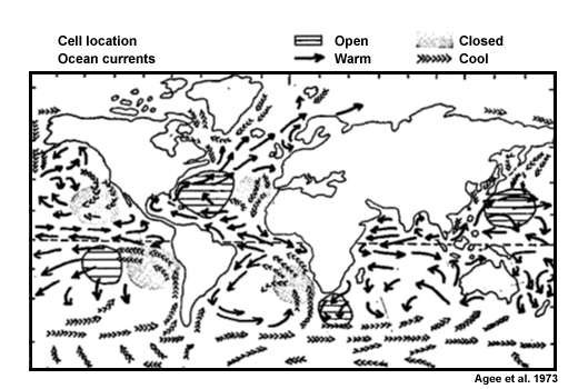
Open and closed cells are favored over certain locations around the globe (Fig. 6.34). For the tropics, closed cells are common to the eastern tropical ocean basins above cool currents, while open cells occur more often over the warmer western ocean currents.69 Both closed and open cells can occur with large-scale sinking motion.70 However, open cells are more common with large-scale descent, while closed cells are more likely with large-scale ascent but sufficiently weak to be limited by the capping inversion.71
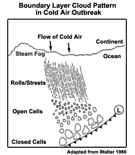
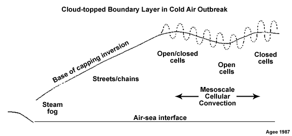
Cloud forms change with distance from the shore during outbreaks of cold air over warm ocean surface in the high-pressure area behind the cold front (Fig. 6.35). Steam fog is usually observed along the coast. Near shore are horizontal rolls or cloud streets followed by mostly open cells and then closed cells immediately behind the cold front. The base of the capping inversion increases farther over the ocean, as the underlying ocean warms the cold air mass (Fig. 6.35 lower).70,72
6.3 The Atmospheric Boundary Layer »
6.3.5 Boundary Layer Clouds »
6.3.5.2 Boundary Layer Clouds and Sub-cloud Characteristics
Thermodynamic environment
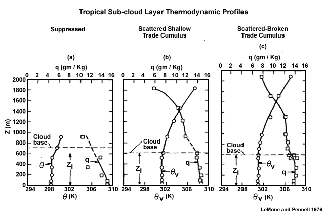
The formation of clouds and the types of clouds depends on the environment and fluxes in the mixed/sub-cloud layer as observed for the tropical marine boundary layer (Fig. 6.36).
- Suppressed regions with mostly clear skies: Marked by linearly decreasing mixing ratio with height and stable conditions in the upper part of the mixed layer (Fig. 6.36a).
- Scattered shallow trade cumulus: Mixing ratio and potential temperature are nearly constant with height in the sub-cloud layer (Fig. 6.36b). The mixing ratio decreases rapidly just above cloud base and continues to decrease more slowly through the cloud. The virtual potential temperature increases nearly linearly with height.
- Scattered to broken trade cumulus: Mixing ratio and virtual potential temperature are constant with height in the sub-cloud layer. Above cloud base, the mixing ratio drops immediately above cloud base but then very slowly decreases through the cloud.
Wind speed and vertical temperature gradient
Boundary-layer convective structure depends on the large-scale vertical motion, wind speed, and vertical surface heat flux, which is a measure of the surface-atmosphere temperature difference (18). By observing changes in the soaring pattern of birds, Woodcock (1942)73 determined how the structure of boundary layer clouds responded to changes in the heat flux and wind speed; whether the clouds would have a roll or cellular pattern (Fig. 6.37). He found that unless the air was cooler than the water, the birds would not soar over the open sea and neither would they soar when the wind speed exceeded 12 m s-1. The birds began soaring when the air-sea temperature difference was enough to generate updrafts to support them.
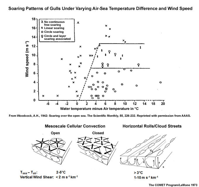
The occurrence of roll clouds, cellular clouds, (Fig. 6.37) or random combinations of the two depends on:
- thermal instability (vertical heat flux to generate convective turbulence) and
- vertical shear in the BL (to organize the convection)
Horizontal convective rolls are prevalent over uniform terrain with moderate surface heat flux and similar wind speed characteristics as over the ocean. The axis of roll clouds is mostly oriented along the mean wind in the CBL. Horizontal roll clouds are wider during cold outbreaks over the ocean and their aspect ratio is dependent on the convective boundary layer height, zi, compared with narrow cloud streets that are more common over land and whose aspect ratio is independent of zi.75
The formation of horizontal rolls or cells can be predicted by a stability parameter, -zi/L,76,77 where L is the Monin-Obukhov length, an approximation for the height at which buoyancy dominates the shear in producing turbulent kinetic energy.
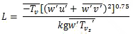 (20)
(20)where k is the von Karman constant, g is acceleration due to gravity, u and v are the horizontal wind components, and w is the vertical velocity. The numerator represents vertical momentum flux and the denominator is the vertical heat flux. In general, for small values of -zi/L, roll convection dominates while for large -zi/L values, free convection or random cells dominate.
Impact of small island or heat island
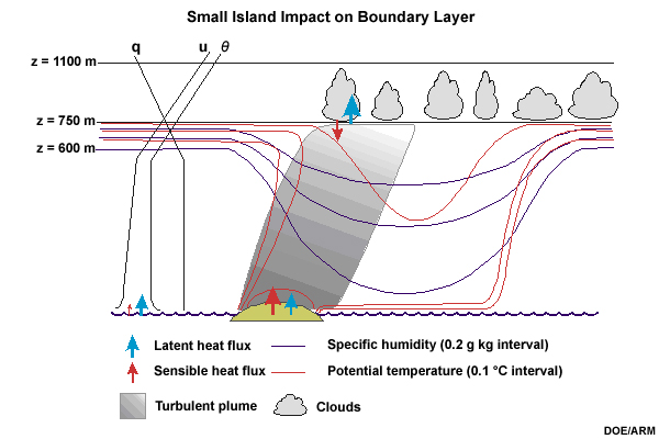
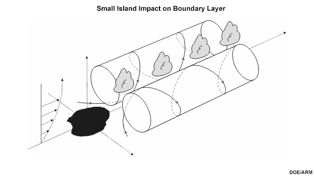
Small islands modify the tropical marine boundary layer including the cloud forms. Figure 6.38 shows how a small island can modify the surface fluxes (increasing the sensible heat flux), generate convective turbulence and thermals that rise to their lifting condensation level (LCL) to produce cumulus clouds within the ABL. Perturbation in the boundary layer air flow can produce convective rolls or vortices downstream of small islands and downstream of urban areas over continents. Long cloud streets could be generated by a pair of convective rolls originating in the convergence zone in the region downwind of a heat island of finite width.78
6.3 The Atmospheric Boundary Layer »
6.3.6 Sub-cloud and Cloud Layer Fluxes and Transport
Vertical transport in the mixed layer is through turbulence during the day, when the surface is usually warmer than the atmosphere. The amount of vertical transport depends on the size and intensity of the turbulent eddies. The growth of turbulent eddies varies with the vertical lapse rate, distance from the surface, and vertical wind shear.79 They are larger and more intense with large surplus surface heating, stronger winds, and highly unstable temperature profile. Thicker mixed layers generally provide more space for the largest eddies to grow. Therefore, the maximum turbulent kinetic energy (TKE) is observed usually during the afternoon in the middle of mixed layer, while the minimum occurs at night.
6.3 The Atmospheric Boundary Layer »
6.3.6 Sub-cloud and Cloud Layer Fluxes and Transport »
6.3.6.1 Fair Weather Mixed Layer Fluxes
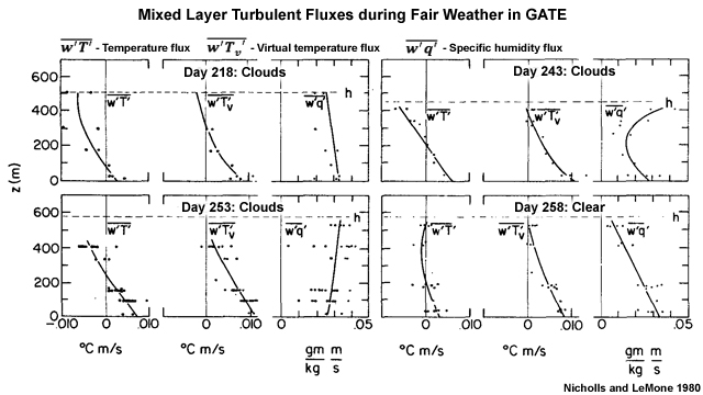 , virtual temperature flux,
  , and specific humidity flux, for fair weather days during GATE. Significant cumulus occurred on (a) Day 218, (b) Day 243, (c) Day 253, no clouds on (d) Day 258. To convert units to W m-2, multiply temperature fluxes by 1150 and humidity flux by 2800.80
A well-mixed boundary layer below non-precipitating shallow cumulus is typical for undisturbed conditions over tropical oceans. Case studies in the tropical Atlantic found that sensible and latent heat fluxes at the top of the mixed layer are strongly influenced by the presence or absence of clouds (Fig. 6.39), i.e., the clouds affected the heating and moistening of the boundary layer even in undisturbed conditions. However, the virtual temperature flux in the mixed layer is similar for all days; showing a roughly linear decrease from the surface to near zero at the top of the mixed layer. On days with shallow cumulus, the overall convergence of water vapor flux in the fair-weather mixed layer is small because the flux at the cloud base is about equal to or greater than the surface flux.80 This indicates that mixing between the cloud base and the mixed layer can remove as much heat as is transferred from the surface. The sensible heat flux convergence is sufficient to offset the loss to radiative cooling (˜2.5K day-1).
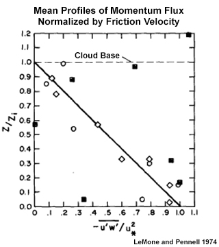
 , normalized by friction velocity, u*2 for observations during GATE.63 Cases of few or no clouds are diamonds; scattered shallow cumulus are open circle; black squares are more active scattered-broken trade cumulus.
The rate of change of momentum flux with height through most of the mixed layer is determined mainly by the shape of the wind profile just above the top of the boundary layer and by the rate of entrainment, and the momentum flux at the surface. During fair weather, the momentum flux decreases linearly from a surface maximum to near zero at the top of the mixed layer (Fig. 6.40), while regions of active broken clouds have no clear relationship.
6.3 The Atmospheric Boundary Layer »
6.3.6 Sub-cloud and Cloud Layer Fluxes and Transport »
Box 6-1 Eddy Diffusivity, Mixing Length, and Turbulent Fluxes
Studies by Prandtl (1925)81 and Taylor (1915)82 established a method of describing turbulent transport as analogous to molecular diffusion, called the eddy diffusivity (ED) theory, also known as the mixing length theory. Vertical turbulent fluxes are assumed to be proportional to the local gradient of the mean profiles of temperature, moisture, and momentum (Section 6.3.1.2Section 6.3.1.2).
A proportionality function, referred to as a K or ED coefficient, is used to describe turbulent fluxes of momentum, heat, and moisture, respectively as:
 (B6-1.1)
 (B6-1.2)
 (B6-1.3)
 (B6-1.4)
where Km, Kh, Kc are the eddy viscosity, eddy diffusivity for heat, and eddy diffusivity for moisture, respectively. Similar formulae can be written for pollutant fluxes.
The K coefficients are prescribed to increase with increasing turbulent kinetic energy. Prandtl parameterized Km as a function of the vertical wind shear, δV/δz, and mixing length, l:
The mixing length, l, the distance over which a parcel loses its identity and is absorbed into the surrounding flow, is estimated by l = k z, where k is the von Karman constant and z is height above ground level.
This method of modeling turbulence in the convective boundary layer has been supplanted in recent years by direct numerical simulation and Large Eddy Simulation (LES) but the eddy diffusivity approach remains a fundamental and useful concept that is employed in many large-scale models.
6.3 The Atmospheric Boundary Layer »
6.3.6 Sub-cloud and Cloud Layer Fluxes and Transport »
6.3.6.2 Vertical Transport and Boundary Layer Clouds
Boundary layer clouds are critical to vertical transport83 and boundary layer physics. For example, latent heat release in boundary layer clouds enhances buoyancy and drives vertical motion.
Heat and Moisture Fluxes
Horizontal roll clouds are an efficient means of vertical transport of heat and moisture across the BL. Within the lowest 70-80% of the boundary layer, the updrafts of roll clouds transport warm moist air upward from the surface. In the upper part of the convective boundary layer and the inversion, the descending parts of the rolls carry warm, dry air from the inversion layer downward74,84 (Fig. 6.41).
Turbulent mixing readily couples cumulus or stratocumulus clouds in the shallow trade wind boundary layer to the surface moisture supply, which comes mainly from the latent heat flux (Fig. 6.39 shows examples of the sub-cloud fluxes). Moisture transport near cloud base results from turbulent transport in individual clouds and mesoscale transport from vertical motions on the scale of the entire cloud layer.63 The upper portions of the cloud layer have net upward moisture flux with maximum downward transport near the base of the inversion. Conversion of the subsiding inversion air into cloud layer air requires cooling and moistening, which may be accomplished by the evaporation of the top of cumulus in the inversion layer.85
Momentum Flux
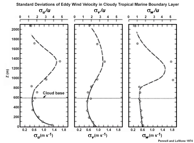
Turbulent kinetic energy (3) in the lowest 200 m above the surface is mainly from mechanical/shear turbulence, which is reflected in the variance of the horizontal and vertical eddy wind components in the cloudy boundary layer (Fig. 6.42). The zonal wind deviation, in particular, decreases sharply above the surface; the meridional wind structure is similar but of smaller magnitude. Both horizontal components slowly decrease to a minimum at cloud base. In this case, the deviation of vertical velocity has a slow linear decay with height. However, other observations found the largest variations in vertical velocity about halfway through the sub-cloud layer.80,86,87 All three profiles peak above cloud base, in keeping with a dynamical response to latent heat release. The profiles are dashed above cloud base to indicate less confidence in observations that were dominated by a few large clouds.
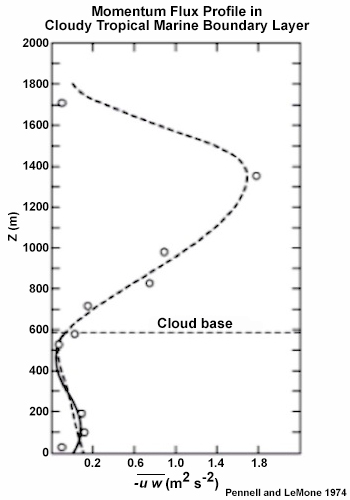
Observations near Puerto Rico found that the eddy flux of horizontal momentum reaches a maximum in the cloud layer, from a minimum about 100 m below cloud base (Fig. 6.43), illustrating the importance of clouds in vertical momentum transport. Note that most of the turbulence observed above cloud base was due to a few, large clouds that changed rapidly. Below cloud base, ˜100 m, both updrafts and downdrafts contribute to the momentum flux63 in the sub-cloud layer. There could be additional momentum flux in the cross wind direction.88
Mass flux
Mass flux transport is particularly critical to cloud microphysics and atmospheric chemistry. A net downward mass flux occurs in the trade regime,89 caused by subsidence in the subtropical anticyclones. The maximum downward transport occurs at the inversion base, the top of the cloud layer. Turbulent fluxes provide some compensating upward mass flux.
6.3 The Atmospheric Boundary Layer »
6.3.6 Sub-cloud and Cloud Layer Fluxes and Transport »
6.3.6.3 Boundary Layer Transport of Chemical Species
Mixed layer properties are critical to air quality assessment, such as the concentration and dispersal of chemical constituents. Additionally, given the vast areas covered by shallow, marine cumulus, we need to consider how they contribute to chemical transport. Exploring the tropical marine boundary layer structure helps us to understand what controls marine aerosol properties as they relate to mixing processes, chemical evolution, and dependence on thermodynamic properties.
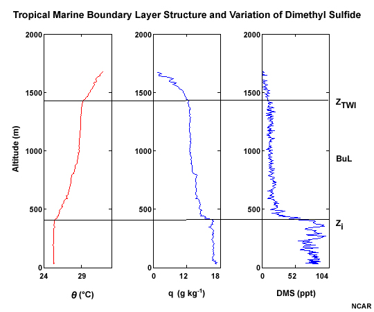
For example, Fig. 6.44 shows the correspondence among profiles of potential temperature, specific humidity, and concentration of DMS, which converts to SO2, an important sulfur gas. The top of a well-mixed layer zi, marks the largest vertical gradient in the thermodynamic and chemical profiles. Above the mixed layer, the concentration of DMS is fairly constant until the top of the trade wind inversion (TWI) when it begins to decrease linearly. Because of turbulent mixing in the MBL and shallow convection, SO2 is continuously depleted by venting into the buffer layer above the MBL. For example, in the eastern, equatorial Pacific, about 57% of the SO2 in the MBL is lost to aerosols, and 27% is subject to dry deposition.90 This type of chemical transport by the tropical MBL helps to improve predictability of marine aerosol concentrations and their impact on the global radiation budget through, e.g., the reflection of solar radiation.
6.3 The Atmospheric Boundary Layer »
6.3.6 Sub-cloud and Cloud Layer Fluxes and Transport »
6.3.6.4 Dust, Smoke, and Haze
Mineral dust is the most abundant aerosol by mass on the globe.91 It affects visibility, air quality (respiratory illnesses, meningitis). It interacts with thermal and solar radiation leading to changes the heating profile and influences cloud microphysics. Large quantities of dust are lifted by synoptic pressure surges, mesoscale downdrafts,92 dust devils, and microscale convective thermals.91,93
Nocturnal LLJs are responsible for a substantial proportion of dust emission over deserts, particularly the Sahara.93 These LLJs form because strong surface radiative cooling creates a nighttime inversion that decouples flow above the inversion from surface friction (section 6.3.2.1section 6.3.2.1). NLLJs in the Western Sahara can have peak winds of 25 m s-1, with the top of the inversion marked by a drop in the water vapor mixing ratio and relative humidity and a significant shift in the wind direction.94
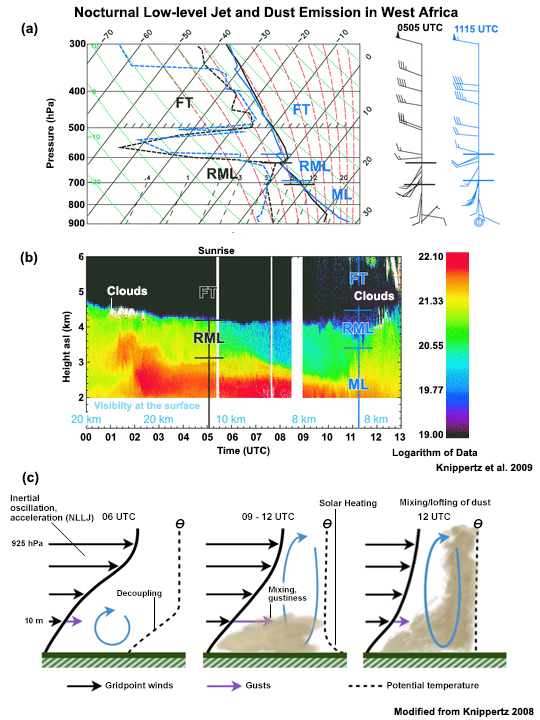
In the Sahara, LLJs peak before sunrise. After sunrise, as the convective ABL grows, momentum mixed down from the jet level generates peak winds at the surface, which raise the dust from morning to about midday95,96 (Fig. 6.45). About 65% of dust emission occurs during this period.97 Notice the reduction in surface visibility as the lofted Sahara dust is carried into the free atmosphere in dry and moist convection (Fig. 6.45b). Plumes of hot air, initiated by elevated heating over the Hoggar Mountains, can inject hot, and likely dust laden air through the Saharan residual layer to altitudes of 8 km. The dust is advected westward to the Atlantic by the prevailing flow; it is the source of half of the mineral dust observed in the Amazon98 forest.
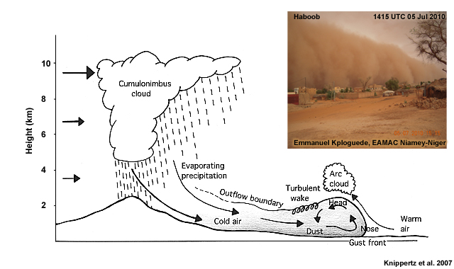
High winds generated by cold outflow from MCSs are a major mechanism for vertical transport of dust (Fig. 6.46). For example, dusty gust fronts or haboobs (Fig. 7.87) caused by MCSs in the Sahel are responsible for a significant portion of dust emission in the southern and central Sahara.96
Gases, smoke, and other particulates from biomass burning are lifted by thunderstorm outflows,100 similar to dust transport. Low-level jets also play a role in the transport of smoke and other pyrogenic products.101 Dry deposition fluxes of soluble species,102 including important plant nutrients, increase during periods of biomass burning (e.g., sugar cane in Brazil103). Larger fires, which are common in the dry season over the Amazon basin, provide vertical transport for aerosols, pollutants, and water from the boundary layer to the mid-upper troposphere.104
6.3 The Atmospheric Boundary Layer »
6.3.6 Sub-cloud and Cloud Layer Fluxes and Transport »
6.3.6.5 Coastal Boundary Layer Interactions and Pollution
In coastal regions, chemical transport becomes more complicated because of the complex topography. Many large tropical cities, which have high concentration of industrial and other air pollutants, are also near the coast. When cool, stable marine boundary layer air moves over hot land, as occurs with the sea-breeze onset, heat is conducted from the hot land to the cool air, leading to convective currents and vertical transport. A thermally unstable lower layer, called a convective internal boundary layer (CIBL) develops. Unmodified stable marine air acts as a capping inversion on the CIBL,5,105 leading to persistent air pollution problems as locally-produced pollutants can be trapped and reach unhealthy levels of concentration near the surface. Pollutants, such as ozone and sulphur dioxides, can be mixed down to the surface by the convective eddies (Fig. 6.47).106
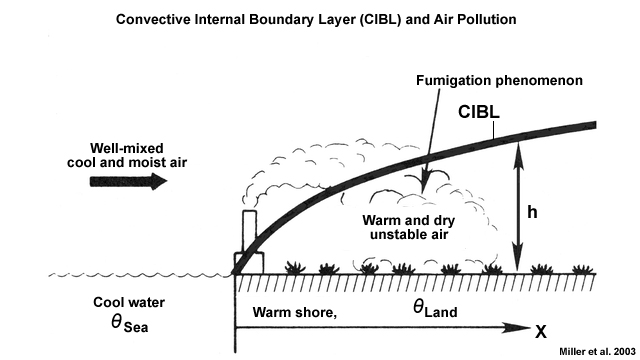
Pollutant plumes can be transported upwards in convective updrafts or near-surface lines of convergence and then conveyed in multiple directions. Plumes caught in the return flow of the sea-breeze, out to the ocean, can be recirculated towards the land and contribute to a growing pollutant concentration as the day progresses.
The CIBL grows to higher levels as the marine air mass moves farther inland; heights of up to 700 m above the ground have been observed in Hong Kong, nearly to the top of its mountains.107 The CIBL will grow more slowly when the marine boundary layer is stable than when it is neutral or unstable. It deepens more rapidly with low wind speeds and greater land surface heating.108
6.3 The Atmospheric Boundary Layer »
6.3.7 The Trade Wind Inversion
The trade wind inversion (TWI) is a prominent, strong temperature inversion that forms in association with subsidence in the subtropical anticyclones, the descending branch of the Hadley circulation (Fig. 3.10b). First documented in 1858 by C. Piazzi-Smyth,18 the TWI was analyzed in detail during the 1927 Meteor expedition.109 It is a persistent feature over large portions of the tropics, e.g., occurring 90-100% of the time between Hawaii and the coast of California. It is typically strongest over eastern tropical ocean basins: the eastern North and South Atlantic, eastern North and South Pacific (near the centers of the subtropical highs, Section 3.2.2Section 3.2.2). A similar inversion was observed over the Bay of Bengal during the pre-monsoon season, but with a higher base than in other ocean basins.48
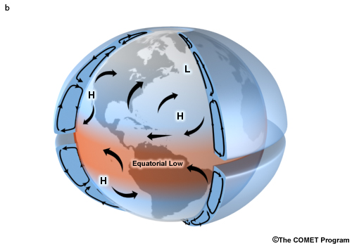
The trade wind inversion limits cloud growth so that the initial movement of sensible and latent heat in the tropics is towards the equator, where vertical transport is concentrated in deep convective clouds in the ITCZ (Fig. 6.1). The inversion affects daily weather and air quality in the boundary layer in the subtropics and into the poleward regions of the tropics; mainly through its influence on stability, clouds, and precipitation.
6.3 The Atmospheric Boundary Layer »
6.3.7 The Trade Wind Inversion »
6.3.7.1 TWI Vertical Structure
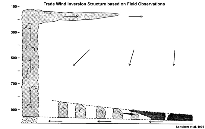
The trade wind inversion is strongest near the center of the subtropical anticyclones, over cold currents, and cool waters upwelled by trade winds blowing away from the subtropical highs. The TWI becomes weaker and its base increases in height with distance towards the west and towards the equator; towards higher SSTs. While most conceptual models (e.g., Fig. 1.18a) show a steep slope in the inversion, observations indicate that the slopes are much more gradual (Fig. 6.48).
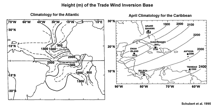
The base of the inversion rises from about 500 m to 2000 m in its westward and equatorward extremes (Fig. 6.49), with a mean slope of about 300 m/1000 km. The inversion layer is about 400 m thick on average but can be as shallow as a few meters and as thick as 1000 m. The lapse rate in the TWI can occasionally exceed 10°C over 1 km. Figure 6.50 shows a typical trade wind sounding, with the inversion base at about 2300 m, corresponding with the drastic drop in relative humidity. The height of the inversion, and hence cloud top, influences the amount of precipitation from boundary layer clouds. Profiler observations from Hilo, Hawaii, found that the TWI varies diurnally by a few hundred meters, with a correlation of 0.7 between the average height of the inversion base and average hourly precipitation accumulations.111
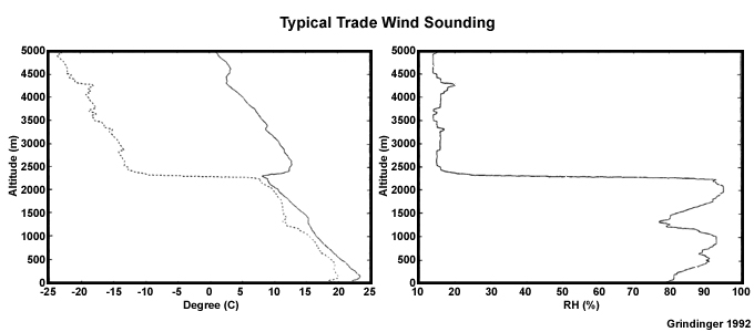
Generally, the tropical troposphere in the trades can be considered as two layers in the wind field, with easterlies at low-levels. Mean soundings from the tropical Atlantic Trade wind Experiment (ATEX) show an easterly wind maximum in the boundary layer with a switch to westerly winds above the inversion (Fig. 6.51).
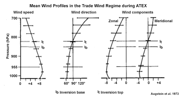
6.3 The Atmospheric Boundary Layer »
6.3.7 The Trade Wind Inversion »
6.3.7.2 Boundary layer clouds and the TWI
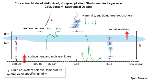
In the east and near the subtropical highs, cool SSTs, near saturation conditions, and light winds in the shallow sub-cloud layer leads to low lifting condensation levels. The subsidence warming and drying results in a large temperature increase above the cloud layer, creating a strong inversion that limits cloud growth (Fig. 6.52). Thus, the typical cloud pattern associated with the TWI has: fog and low stratus near the coast, stratocumulus offshore, and cumulus over the relatively warm open ocean. In the coastal, low-inversion region, precipitation occurs mostly as light drizzle from stratus clouds. Farther offshore, in the region of stratocumulus cloud, clouds are thicker. Even farther west, with the weaker TWI and higher inversion base, trade cumuli are thicker, drizzle is frequent, and convective precipitation is observed.
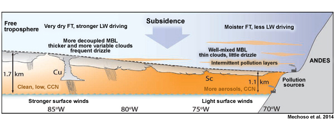
The transition from closed stratocumulus layer to open trade cumulus is presented conceptually in Fig. 6.53. As surface fluxes increase with warmer SSTs, the mixed layer depth increases, and the stratocumulus cloud layer becomes decoupled from the surface mixed layer. Turbulence increases within the cloud layer, leading to the formation of cumuli, which start to entrain through the inversion. Drying due to entrainment evaporates the stratocumulus layer.112
The TWI structure also affects aerosol transport (Fig. 6.53). In the east (along western coasts) are high concentrations of CCN from cities and industrial sources, leading to higher droplet concentrations but little or no precipitation (Chapter 5, Section 5.3.2Chapter 5, Section 5.3.2). Farther west, taller precipitating cumulus occur with a weaker inversion, higher base, and cleaner air but fewer CCN.
6.3 The Atmospheric Boundary Layer »
6.3.7 The Trade Wind Inversion »
6.3.7.3 Formation and Maintenance of the TWI
The TWI is a stable layer, which means that its formation and maintenance are dependent on factors that lead to increasing potential temperature with height (see the stable layer in Fig. 6.4b).
- The most important factor that contributes to increasing the static stability is strong divergence away from the subtropical ridge. The inversion weakens as divergence weakens to the west.
- Another mechanism that maintains the inversion in the east is the sensible heat flux. The air is warmer than the cold ocean currents and upwelling water, thereby establishing an inversion near the surface. Warmer SSTs to the west, lead to more instability and a weaker inversion.
Clouds act to destabilize the inversion. At cloud top, long wave emission leads to radiative cooling, while emission from beneath the cloud contributes to radiative heating. The combination of radiative processes weakens the inversion. Turbulent heat fluxes within clouds increase vertical mixing of high potential temperature air above the cloud and low potential temperature air at the cloud base, which acts to weaken the inversion.
The TWI is more uniform than the local values of divergence and SSTs, temperature and moisture above the inversion would suggest, indicating that the TWI height is strongly coupled to the horizontal averages of the divergence, SSTs, and thermodynamic structure above the inversion.110
6.4 Vertical Transport in Deep Convection
Deep convective clouds are the main conduit for the vertical transport of energy, moisture, momentum, and chemical constituents in the tropical troposphere. Tropical clouds fit mainly into three categories: boundary layer stratocumulus and cumulus, cumulus congestus, and cumulonimbus (Fig. 5.10). While shallow moist convection is the most commonly observed state of the tropical skies (Fig. 6.32), vertical transport is greater in the smaller areas of precipitating deep convection (Fig. 6.54) and its associated processes have a greater impact on large-scale circulations.
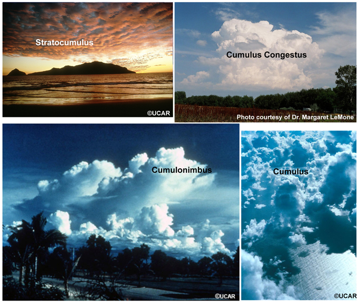
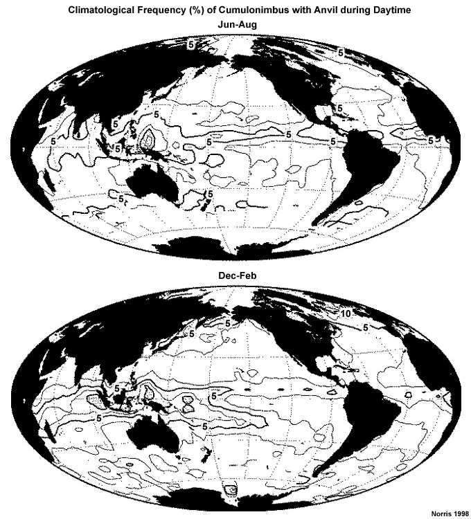
6.4 Vertical Transport in Deep Convection »
6.4.1 Growth of Cumulus Clouds
Tall cumulus and cumulonimbus, so called hot towers (Section 1.2Section 1.2), are the primary means for delivery of energy from the surface to the upper troposphere (Fig. 6.1). Buoyancy is the primary mechanism that forces the growth of cumulus clouds (Box 5-3Box 5-3). Air that is warmer (less dense) than the environment will rise (Section 6.3.1.1Section 6.3.1.1).
6.4 Vertical Transport in Deep Convection »
6.4.1 Growth of Cumulus Clouds »
6.4.1.1 Ordinary Cumulus Growth in the Free Atmosphere
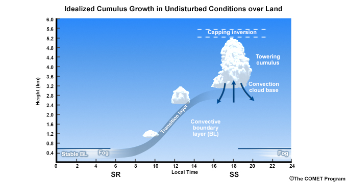
For the undisturbed conditions over land, the typical diurnal cycle will evolve as shown in Fig. 6.55 with small, shallow clouds giving way to deeper clouds (cumulus congestus) as the surface warms and convective turbulence increases and the mixed layer grows in the afternoon (at a rate of 10 cm s-1). After sunset, the clouds decay as convective turbulence ceases and the surface cools rapidly, and the surface is decoupled from the rest of the boundary layer. With sufficient relative humidity, fog forms in the shallow, stable, nocturnal boundary layer.
6.4 Vertical Transport in Deep Convection »
6.4.1 Growth of Cumulus Clouds »
6.4.1.2 Cloud Evolution in Tropical Disturbance
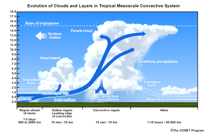
With disturbances such as a tropical squall line, complex interactions occur between the surface, the boundary layer, and clouds in the free troposphere (Fig. 6.56). Vertical mixing occurs through the depth of the troposphere. Strong updrafts help to transport surface air and its related properties to the upper troposphere and even into the lower stratosphere. Tilting front-to-rear updrafts originate from the sub-cloud layer (~15%) and mid-troposphere (~ 75%). Rear-to-front mesoscale downdrafts bring mid-tropospheric air to the surface almost undiluted. Convective outflow triggers new cumuli ahead of the storm.
The vertical and time evolution can be divided into:
- The region ahead of the storm where the surface and turbulent heat fluxes have been building up over 1-3 days, with a capping inversion at about 1 km.
- The narrow leading convective edge where new cells have broken through the inversion after being lifted by the outflow from the parent storm.
- A convective region with strong updrafts and heavy precipitation connecting the surface with the upper-troposphere. The result is a deep layer of well-mixed neutrally-stratified air.
- A trailing stratiform rain and wake region that lasts for 1-10 hours. Mesoscale downdrafts warm and dry the air in the wake, suppressing the mixed layer. The shallow mixed layer cannot support new convection.
This evolution helps to explain the quasi 2-day periodicity for tropical squall lines observed in the tropical west Pacific113,114 and tropical Africa.115
For strong squall lines, the system survives by maintaining a balance between the cold pool vorticity and the vertical shear that allows the updraft to be separated from the downdrafts. By propagating at the same rate as the density current, some tropical squall lines last for 24-48 hours.
6.4 Vertical Transport in Deep Convection »
6.4.1 Growth of Cumulus Clouds »
6.4.1.3 Simple Buoyancy Model
Simple buoyancy models are useful for helping us understand convection and vertical motion. Consider an air parcel in a neutral environment (constant potential temperature with height) over dry land. As the surface heats, dry convection starts in the surface layer, which has a super-adiabatic lapse rate. The thermal acts to destroy the super-adiabatic lapse rate. This dry convection process can be represented in a simple model where the pressure and density are separated into a mean and perturbation state,  and
and  .
.
With hydrostatic balance,  . But when considering the perturbation contribution, a buoyant parcel with density, ρ′, would accelerate vertically according to:
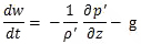 (21)
(21)Assuming pressure continuity across the rising parcel and substituting for density using the equation of state, p=ρRTv, where Tv is the virtual temperature and R is the gas constant for dry air, then the vertical acceleration of the parcel due to buoyancy can be expressed as:
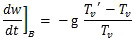 (22)
(22)In other words, the buoyancy contribution to the vertical acceleration of an air parcel is a function of the difference between the parcel temperature and a basic hydrostatic state.
Question
The sounding below represents the following conditions: (Choose all that apply.)
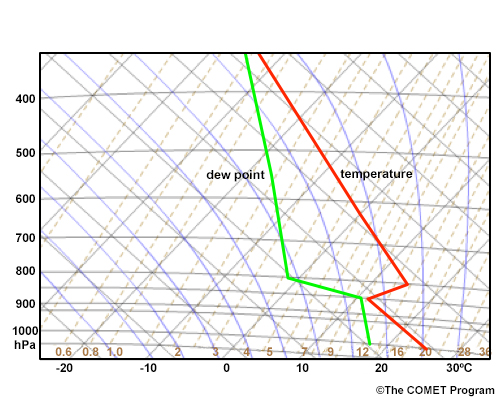
The correct answers are d and h.
The sounding is of a moist, mixed layer, of 100-150 hPa in depth, capped by an inversion. The temperature decreasing at the dry adiabatic lapse rate is typical for the mixed layer over land during the daytime. With surface heating, the inversion could be eroded, resulting in intense convection. For that reason, this type of sounding is referred to as a loaded gun.
6.4 Vertical Transport in Deep Convection »
6.4.1 Growth of Cumulus Clouds »
6.4.1.4 Cumulus Impact on the Sub-cloud Layer
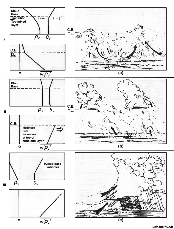
The sub-cloud layer becomes increasing stable as convection becomes more intense and the clouds become taller and more widespread (Fig. 6.57).
(i) Beneath fair weather boundary layer cumulus, the sub-cloud layer is statically neutral. The specific humidity is constant throughout most of the mixed layer then decreases linearly through the transition layer. The eddy moisture flux decreases linearly with height.
(ii) As the clouds increase in depth and amount, the specific humidity and virtual potential temperature are constant in the mixed layer. However, the surface layer is super-adiabatic. Eddy moisture flux increases at the top of the mixed layer.
(iii) During the passage of a weather disturbance, such as a tropical squall line, the temperature and humidity drop sharply. Cool downdrafts replace unsaturated air below cloud base and liquid water, in air descending from above the cloud base, evaporates. This cool and shallow mixed layer persists for several hours over the tropical oceans, maintained by continuing downdrafts. The eddy moisture flux now increases with height. The sub-cloud layer of moderate or heavily precipitating cumulus is about 1K cooler and 1 g/kg drier than the unmodified air. This stabilization means that new convection is limited until the boundary layer recovers to its undisturbed state.
6.4 Vertical Transport in Deep Convection »
6.4.2 Cumulus Heat and Moisture Budgets
Heat and moisture transport by cumulus has a strong effect on the large-scale dynamics of the atmosphere. As first pointed out by Riehl and Malkus (1958),1 concentrated upward heat transport in tropical cumulonimbus (hot towers) is required to balance heat loss in the upper troposphere from radiation and poleward transport. Heat gets to the top of the troposphere in just hours via convection compared with days via radiation at optically thick wavelengths. The overall effect of precipitating cumulus clouds is to warm and dry most of the troposphere through condensation/evaporation and eddy transports.
On large horizontal scales, convection is in quasi-equilibrium with the large-scale forcing. Study of the vertical transport of heat and moisture is framed within an ensemble of cumulus clouds embedded in large-scale motion (Fig. 6.58), with heat sources and heat sinks.
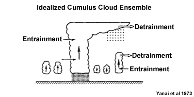
With adiabatic vertical motion, dry static energy, s, and moist static energy, h, are approximately conserved (Section 5.2.3Section 5.2.3). However, neither is conserved in the presence of diabatic processes, instead the derivative of the static energy is a function of the diabatic heating rate itself a product of the net radiation and net latent heating in the troposphere. Then, according to Yanai et al. (1973),116 the energy budget may be partitioned into contributions from heat sinks and heat sources, which are computed from sounding data:
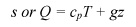
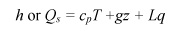
Q1 = Apparent Heat source (sensible and latent heat), heating rate in °C or K per day
The diabatic heating/cooling rate calculated as a residual of the energy budget(23)
Q2 = Apparent Moisture sink (latent heat), °C or K per day
The rate of moistening/drying (in terms of water vapor addition or removal, respectively), is traditionally also couched in the form of an equivalent heating rate, with heating expressed in terms of "cumulus drying" and cooling representing "evaporative moistening".(24)
where q is the water vapor mixing ratio; other variables are described above. In highly convective cases, the eddy vertical flux contributes significantly.
Ignoring the horizontal eddy transport, then,
(25)
where the moist static energy, h= cpT + gz +Lq (Section 5.2.3Section 5.2.3).
Equation (25) has been used to measure the activity of cumulus convection,116,117 the vertical distribution of heating, and the effect of cumulus on the heat and moisture budgets of different regions in the tropics.
By integrating Equations (23) and (24) from the surface to the tropopause, we can relate the tropospheric diabatic heating to the precipitation rate (R), evaporation rate (E), and sensible heat flux,118 (S), per unit area at the surface, as:
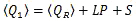 (26)
(26) (27)
(27)where ⟨ ⟩ is the integral from the surface to the tropopause.
Combining (26) and (27), we get
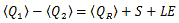 (28)
(28)Using the relationships above, in combination with the outgoing longwave radiation (OLR) distribution, we can:
- interpret heat budget results,
- evaluate the consistency of the Q1 and Q2 estimates, and
- determine the effect of the diabatic processes on the horizontal distribution of the vertically integrated heating.
For example, if heating is due to deep cumulus condensation then Q1 is nearly equal to Q2 and QR would be small. Alternately, with strong surface evaporation or sensible heat flux, then the horizontal distribution of Q1 would be very different from Q2.
6.4 Vertical Transport in Deep Convection »
6.4.2 Cumulus Heat and Moisture Budgets »
6.4.2.1 Horizontal Distribution of Vertically Integrated Heating
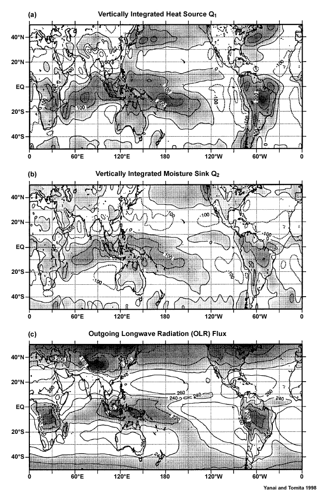
The vertically integrated heating distribution across the tropics has a seasonal cycle that is consistent with the observed mean tropical circulations. This is supporting evidence for diabatic heating as the driver of most tropical circulation.
During December to February, large maxima of both Q1 and Q2 occur over the southern tropical continental areas, warm ocean basins, and the South Pacific Convergence Zone (Fig. 6.59). The coincidence with minima in QR means that most of that heating is due to condensation in deep convection. Meanwhile the large negative values of Q1 and Q2, representing heat sinks and moisture sources, respectively, are found over the subtropical continents and eastern oceans. There, negative Q2 is due to strong surface evaporation exceeding precipitation (27) and for negative Q1, radiative cooling exceeding sensible heat flux and latent heat flux (26).
During spring in the northern hemisphere, subtropical regions in Asia and North America are major heat sources, with high values of Q1 and low values of Q2, which can be attributed to sensible heat flux as a primary contributor to the vertical heating. During September to November, the heat sources are relatively weaker. The eastern subtropical oceans remain as heat sinks, similar to other seasons.
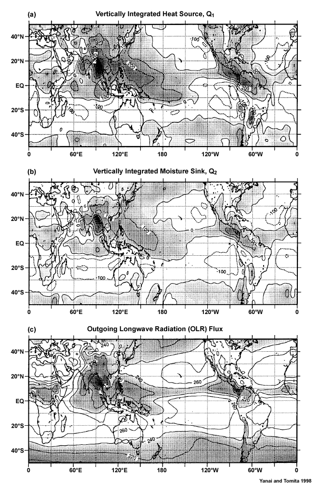
For June to August, the main heat sources are northern tropical continents (Africa and Asian monsoon regions), the tropical western Pacific, and around Central America (Fig. 6.60). The heating over the continents is dominated by sensible heat flux, as Q2 is small compared with Q1. Over the tropical oceans, where the two are large and nearly equal and QR is small, the implication is heating from condensation in deep cumulus convection. The heat sinks of the subtropics and eastern tropical oceans are similar to December to February except for being more prominent in the Northern Hemisphere.
As noted in Chapters 33 and 44, the vertically integrated heating pattern at or near the equator induces large-scale atmospheric flows, such as equatorial waves (Section 3.4Section 3.4), which can be estimated by using the shallow water equations of motion. In general, tropical circulation features (Fig. 3.14), such as the equatorial/monsoon trough, oceanic subtropical highs, trade winds, and heat lows over subtropical continents during summer, can be diagnosed as a response to the apparent heat sources and sinks in the tropics and sub-tropics. Vertical transport in the Hadley cells is critical to meridional transport, while vertical transport in the Walker Circulation is responsible for zonal transport (Fig. 3.28).
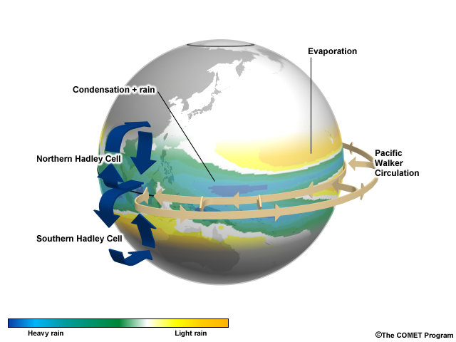
6.4 Vertical Transport in Deep Convection »
6.4.2 Cumulus Heat and Moisture Budgets »
6.4.2.2 Vertical Distribution of Diabatic Heating
The vertical distribution of diabatic heating can also be used to interpret the contribution of different cloud processes. Heating from condensation in stratiform clouds will have similar vertical profiles of Q1 and Q2 while condensation with cumulus will produce different profiles of Q1 and Q2 with maxima at different levels of the troposphere. Additionally, if surface sensible heat flux is the main heat source, such as occurs above dry surfaces during daytime, then Q2 will be negligible.
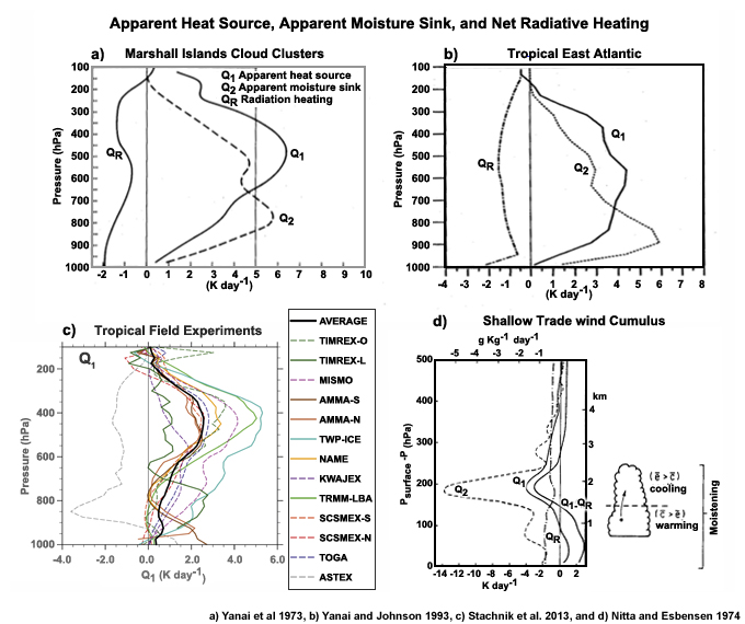
Heating profiles vary among cumulus convection in different tropical regions (Fig. 6.61) but most have a broad maximum heating rate, Q1, between 500 and 400 hPa (2-6 K day-1). The average Q2 has a lower maximum near 700 hPa and a secondary peak near 500 hPa. The double peak structure is due to the combined contributions of convective and stratiform components of organized convective systems. The difference between the profiles indicates the effect of eddy vertical transport of moist static energy by cumulus convection (25). For cloud clusters over the tropical East Atlantic, Q1-Q2-QR is positive in the upper troposphere and negative in the lower troposphere.
Shallow trade wind cumulus has maximum warming below cloud base and peak cooling and moistening in the shallow cloud layer (at about 200 hPa above the surface, Fig. 6.61d). Above that level, heating and cooling are near zero.
Most tropical convection is organized on the mesoscale (length 100-1000 km, time hours day). For mesoscale convective systems, the heat budget can be divided into its cumulus/convective (Q1c, Q2c) and mesoscale stratiform (Q1m, Q2m) components:
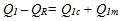 (29)
(29) (30)
(30)These quantities reflect the time and space average effect of convection (unresolved scale in grid models) and stratiform heating/drying (resolved scale in grid models).
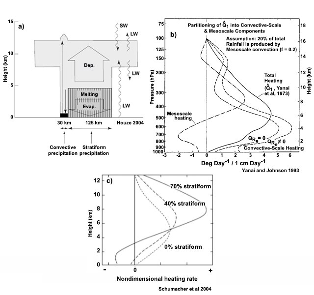
Net heating results from latent heat released during condensation (Fig. 6.62). The intense but smaller convective region has updrafts from the boundary layer up to the equilibrium level and precipitation downdrafts only in its lowest levels. The stratiform region has a large region of ascent above and downdrafts below the melting layer (Fig. 6.62a). The resulting stratiform profile has warming above and cooling below due to melting and evaporation beneath cloud base (Fig. 6.62b,c). The net heating in MCSs is concentrated in the middle to upper troposphere because of how the convective and stratiform regions are arranged. The stratiform precipitation region exerts great influence on the overall vertical heating profile; the larger the percentage of stratiform region in an MCS, the higher the level of maximum heating (Fig. 6.62c). In general, the presence of an MCS implies overall heating of troposphere with the heating maximum in the upper troposphere. Midlatitude MCSs generally have a sharper peak in heating and at a higher level than tropical MCSs. In the equatorial regions, MCSs tend to accumulate heating in the upper troposphere, with a small net heating at lower levels.
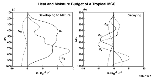
Not surprisingly, moisture and heat budgets vary according to the degree of convective activity over a diurnal cycle or through the lifecycle of an MCS. Figure 6.63 shows the variations in the budgets between a GATE cloud cluster during developing to mature conditions and decaying conditions. During the mature stage, Q1 peaks in the middle to upper troposphere (~400 hPa), while Q2 peaks in the lower troposphere (~750 hPa). At the decay stage, the Q1 and Q2 are smaller in magnitude and have complicated vertical structures compared with the mature stage. Q1 becomes negative (a heat sink) in the mid-troposphere. The heat source maximum is in the low troposphere, near 900 hPa. Q2 is largest near 850 hPa during the decay phase, with a negative peak near 650 hPa. Heating profiles correspond to strong upward eddy heat flux during the developing and mature stages of MCS lifecycles, moderate upward flux during undisturbed conditions and weak fluxes during the decay stage.
Differences are found between the tropical east Atlantic and tropical west Pacific. Generally, maximum heating in western Pacific MCSs occurs in the middle to upper troposphere (~450 hPa) during the mature-to-decaying stages while GATE systems experience maximum heating earlier and lower in the troposphere.124
Vertical Velocity in Deep Convection
Recall from Chapter 3Chapter 3, that when the thermodynamic energy equation is scaled for low latitudes, the result is that in the absence of strong diabatic heating, horizontal temperature advection is balanced by vertical motion with vertical velocity ~ 0.3 cm s-1. With strong diabatic heating in deep convection, the heating rate is about 5 K day-1, which requires vertical velocity of 3 cm s-1.
6.4 Vertical Transport in Deep Convection »
6.4.3 Convective Mass Flux
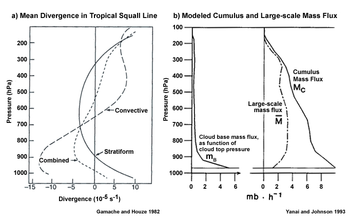
 (dash-dotted). Cumulus mass flux peaks near the surface and decreases with height.117
Convective updrafts ingest air from the most unstable layers and detrain air at cloud top (level of neutral buoyancy). Downdrafts in deep convection are initiated in the middle troposphere and bring concentrated doses of low energy air from the low-to middle troposphere to the low troposphere and surface (Fig. 7.91). Moist downdrafts also detrain cloud water and transport heat and moisture. With descent, the air is adiabatically warmed and dried. Balancing the mainly upward convective mass flux is compensating downward flux between clouds; this is the main way in which cumulus modifies the large-scale environment.
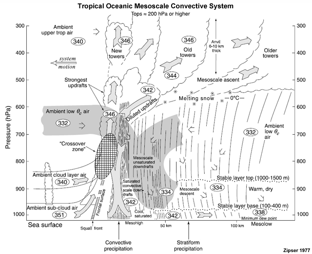
Mass flux in tropical deep convection occurs in association with strong low-level convergence and upper-level divergence (Fig. 6.64). Mass transport due to cumulus convection is important to cloud microphysics and atmospheric chemistry. Convective mass flux, an important component of convective parameterization, needs to be realistically determined in order to predict the redistribution of particles in the atmosphere.126 Convective mass flux is diagnosed from heat and moisture budgets,127 described in the previous sectionprevious section. Numerical models must be able to represent Q1 and Q2 as functions of resolved variables, a process is known as parameterization.
6.4 Vertical Transport in Deep Convection »
6.4.4 Momentum Transport in Deep Convection
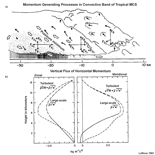
 and
and  , solid and dashed lines) and the large-scale flow (
 and
and  , dashed and dot-dashed lines) in a 140 km plane perpendicular to the squall line depicted in (a).128
The vertical transport of horizontal momentum can be quite different when cumulus is organized into lines than when convective clouds are isolated or more or less randomly distributed. As discussed earlier regarding vertical momentum transport, the simple assumption is that, when wind speed increases with height, downward-moving air parcels would be bring high momentum down (down the vertical gradient) and upward-moving parcels would carry low momentum.
However, vertical transport that is perpendicular to a tropical squall line can be "upgradient" (enhancing the mean flow and working against the vertical momentum gradient), while the line-parallel transport is "downgradient" (the simplified mixing process).128,129 Momentum flux is generated in the narrow, growing convective updraft. Air flowing into the convective cloud base is accelerated upwards by buoyancy and rearwards by a meso-low in the rear of the squall line (Fig. 6.65). The configuration of a tilted updraft with a pressure minimum below is consistent with the idea that cross-line momentum is removed from lower levels and added to the upper levels. Air leaving the upper levels has greater momentum than when it entered, resulting in profiles of vertical momentum flux that peak in the upper levels (Fig. 6.65b). Tropical squall lines are major contributors to the large-scale vertical momentum transport.
6.4 Vertical Transport in Deep Convection »
6.4.5 Chemical Transport in Tropical Deep Convection
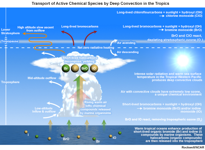
Once in the free atmosphere, trace gases rise through deep convection (Fig. 6.66), which couples the surface, the boundary layer and the free troposphere. Air from the boundary layer can reach into the tropical tropopause layer (TTL) in a few hours.130,131 However, only a small fraction of deep convective clouds penetrate directly into the lower stratosphere.132 As described in Section 3.2.4.1Section 3.2.4.1, the TTL is a layer of transition between the upper troposphere and the lower stratosphere.133 Deep convective clouds influence the exchanges with the stratosphere through their interactions with the TTL (Fig. 3.18a). Chemical species and water vapor enter the stratosphere from the TTL.134
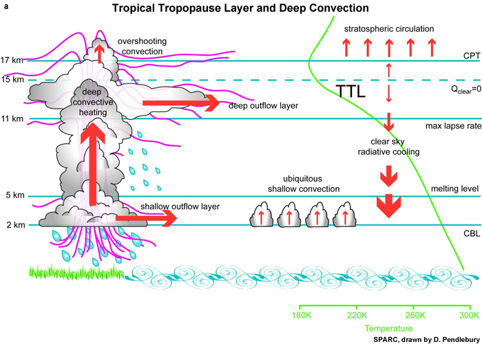
6.4 Vertical Transport in Deep Convection »
6.4.6 Modeling Cloud Processes and Effects
Tropical clouds present a challenge to numerical models because they occur on a wide range of spatial scales, although most tropical convection is organized at the mesoscale. Cumulus clouds occur at time scales that are too small and too short to be represented explicitly.135 Cloud resolving models with horizontal grids small enough (4 km or less) to resolve large convective clouds and mesoscale cloud structures have become more common since the 2000s.136,137 However, global and regional models still use various parameterization schemes to formulate model sub-grid scales and eddy transports due to the broad range of cloud processes and scale.
In order to design realistic models of cloud effects and cloud systems, we need to understand vertical transport, cloud growth, and related sub-cloud and cloud processes. This pursuit has preoccupied the atmospheric sciences for several decades.135,138 In recognition that this continues to be an active research area, we focus only on some basic concepts that are applied in modeling tropical clouds and their effects including cumulus parameterization, cloud resolving numerical models, and multi-scale modeling frameworks.
6.4 Vertical Transport in Deep Convection »
6.4.6 Modeling Cloud Processes and Effects »
6.4.6.1 Conventional Cumulus Parameterization
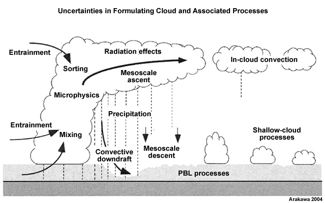
Major uncertainties in formulating clouds and associated processes are illustrated in Fig. 6.67. Cumulus parameterization schemes are formulated to represent the sub-grid scale effects of cumulus convection,139,140,141,142 the statistical effects of cumulus clouds, without predicting individual clouds. They are designed to determine:
- Vertically integrated cumulus heating (Section 6.4.2Section 6.4.2), a fundamental objective, as it determines whether and how much cumulus activity will exist under given synoptic conditions. It is also closely associated with the prediction of surface precipitation, one of the most important weather and climate variables.
- Vertical distribution of cumulus heating/cooling and drying/moistening (Section 6.4.2.2Section 6.4.2.2), which drives the general circulation in the tropics.
Convection schemes have a closure assumptiona main hypothesis that relates the occurrence and intensity of sub-grid cumulus convection to resolved processes. For example, the Arakawa-Schubert scheme requires that deep convection reduces instability on the timescale of a diurnal cycle and, in that process, drives the moist static energy of the upper layer toward that of the boundary layer. It accounts for moisture detrainment from clouds and warming from subsidence (Fig. 6.68). Section 9.4.6Section 9.4.6 reviews cumulus convection in NWP, including the closure assumptions of some commonly-used convection parameterization schemes.
Generally, deep convection is parameterized and not predicted explicitly for grid spacing below 10 km143,144 because as grid spacing decreases, the conceptual basis for the parameterization becomes more ambiguous.138 Cumulus convection schemes seek to quantify the eddy transport from convection not the total transport. Errors occur in models if the grid (resolved) scale and eddy transports are not distinguished clearly; the convection scheme may count the same effect twice or create spurious competition between the sub-grid and grid scale values.
Convection parameterization in global models
Major improvements have been made in representing convection in global models since the reviews done in the early 2000s,138,145 particularly in representation of entrainment and convective organization.146,147 The movement has been towards unified modeling of cloud processes and resolution independent parameterization. Most conventional cumulus schemes make assumptions about the fractional area covered by convective updrafts (σ), where σ « 1 in a global model grid box. The thermal structure of the cloud environment is defined using the grid-point values of thermodynamic variables and parameterization is regime dependent. For grid spacing of 100 km, updraft fraction is small but for high-resolution models, 10 km, the updraft fraction can be of order 1.
One unified parameterization approach differentiates between the given gridpoint values and the hypothetical environmental values.148 The ratio of eddy transport to total transport is shown to depend on the updraft fraction but not on the grid spacing. The total transport is due to eddy transport for small values of updraft fraction and mostly by grid-scale transport for large updraft fraction.
Another unified model has been implemented in the NCAR Community Atmospheric Model149 (CAM). Rather than regime dependent parameterization, this approach is process-dependent (Fig. 6.69). With this process-dependent parameterization, a moist turbulence scheme accounts for the local transport, simulating both dry and saturated turbulent transport in all atmospheric layers using one set of moist physics formulae. The non-local transport is done by UNICON, including sub-grid convective updrafts from the surface (starts out unsaturated but becomes saturated above the LCL) and convectively generated downdrafts that can penetrate into the ABL.
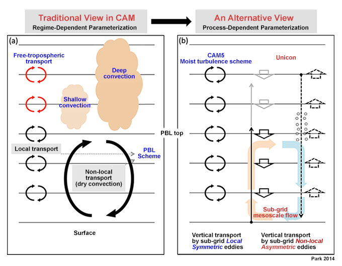
Rather than having vertical transport of moisture and other conserved scalars be handled by advection, ABL, and convection parameterizations, this scheme parameterizes sub-grid vertical transport by non-local asymmetric turbulent eddies (relative to the mean grid vertical flow). In the unified model in CAM, shallow moist convection warms the cumulus layer, transports moisture from the lower to the upper tropospheric cumulus layer, and condensate is detrained to any cumulus layer height.
Convective parameterization is covered in detail in the COMET module, How Models Produce Precipitation and Clouds, http://www.meted.ucar.edu/nwp/model_precipandclouds/.
6.4 Vertical Transport in Deep Convection »
6.4.6 Modeling Cloud Processes and Effects »
6.4.6.2 Cloud Resolving Models
As computing capacity has increased, NWP has been conducted at increasingly higher resolution with mesoscale models now allowing convective overturning to be an explicitly resolved process. Precipitation is produced using explicit microphysics at each grid point. Introduced in the 1990s, cloud-system resolving models (CSRM) were first applied to modeling tropical convection in climate models because they allow explicit interactions between cloud microphysics, cloud dynamics, radiation, ocean and land surface processes.136
CSRMs include more sophisticated cloud microphysical processes and resolve the structure and lifecycle of clouds and mesoscale characteristics of convection (depending on the spatial resolution).150 While grids of ~5 km can produce realistic time evolution and structure of mesoscale convective systems, that scale is more accurately described as cloud-permitting. To be convection-resolving, models need horizontal grid spacing on the order of 100 m in order to resolve turbulence in the clouds, including the entrainment process that is an inherent part of convective overturning.151,152 For convection driven by land surface heating, accurate prediction of the timing and intensity of convection seems to need spacing below 1 km to resolve boundary layer eddies that initiate convection.153
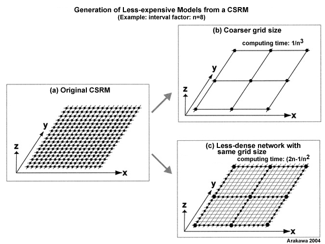
Global CSRMs can resolve (or "permit") large convective clouds and mesoscale convective structures (Fig. 6.70a) but are computationally expensive.135 CSRMs can be embedded into global models to help to quantify interactions between the mesoscale and large-scale motion, cloud-climate interactions, and aerosol-cloud-precipitation interactions. The method shown in Fig. 6.70(c) saves on the computational requirements of a global CSRM. The model will only be fully 3D at the widely spaced grid points but the smaller grid values can have bogus values based on interpolation or regression. This model will be able to deduce gross 3D structures of cloud organization within a network.
6.4 Vertical Transport in Deep Convection »
6.4.6 Modeling Cloud Processes and Effects »
6.4.6.3 Superparameterization
Since the early 2000s, an approach called superparameterization has been applied to global atmospheric modeling. A superparameterization takes a simplified CSRM with a 2D domain and periodic lateral boundary conditions and copies the CSRM into each grid column of a conventional global climate model.145 This combination is called a Multiscale Modeling Framework (MMF).154
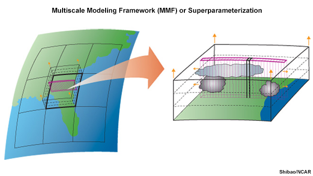
The CSRM consists of a set of columns spaced about 4 km apart inside each global model column (Fig. 6.71). Each CSRM runs continuously and independently; no communication between them. While the CSRM does not really resolve clouds, it uses appropriate fundamental equations to describe basic cloud dynamics rather than the simpler formulations used in traditional global models.135
6.5 Synthesis: From the Surface to the Tropopause
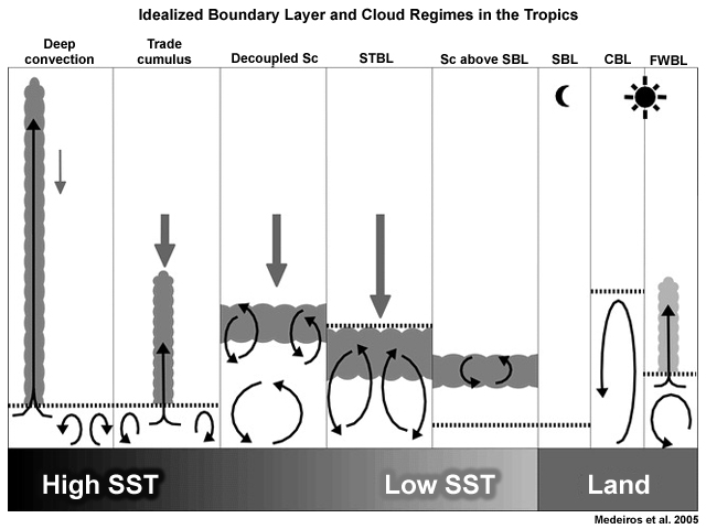
The general circulation of the atmosphere involves various processes whose role is to help the atmosphere to return to an equilibrium state, where energy and momentum are balanced globally. The vertical transport component of tropical circulations results from deep convection and shallow convection, which operate at different time scales.
In the journey from the surface to the troposphere, energy and momentum and atmospheric constituents travel through many layers and are involved in many processes. Figure 6.72 shows several idealized cloud and flow regimes in the tropical troposphere.
The most rapid and impressive vertical transport occurs in the deep cumulus convection over warm SSTs, driven by strong surface fluxes of latent and sensible heat, instability and buoyancy in the boundary layer. Accompanying the dramatic updrafts in organized deep convection is compensating subsidence in cloud free regions. Trade cumuli occur in the cumulus-coupled boundary layer, which has surface forcing from warm SSTs and strong updrafts into individual clouds.
The shallow stratocumulus/cumulus regime is a complicated but common regime over the tropical oceans. The shallow convection layer occupies the lower third of a subsiding stratified troposphere and exists above a sub-cloud layer, where sensible heat flux convergence balances radiative cooling as turbulent eddies distribute surface heat at a faster rate than is lost to cooling processes. Cloud depth decreases eastward and poleward with increased subsidence from subtropical highs, increased divergence, and lower SSTs. Farthest east and poleward, the stratocumulus topped boundary layer is sustained by transport in active convection, which is due to conditional instability between the upward heat flux and radiative cooling at cloud top. In this region of low SSTs and subsidence warming above, the marine boundary layer is stable with a low inversion.
Over land, the convective boundary layer is relatively deep due to strong surface heat fluxes, allowing large eddies to transport energy to higher levels than occurs over ocean or at night. The largest eddies in the CBL have time scales of about 15 minutes, so the entire BL overturns in less than a day. When rising thermals reach the LCL, cumulus forms and grows in the late afternoon. As cumulus convection becomes more intense, the cloud base lowers and the sub-cloud layer becomes more stable. With cooling of the surface after sunset, a shallow stable boundary layer, with a surface inversion, is established and vertical transport is limited.
Focus 1: Modeling the Tropical Boundary Layer
The tropical boundary layer is critical to weather and climate as it serves as the conduit for surplus energy from the tropical surface to deep convection and the Hadley circulation, and to higher latitudes. It also serves as a critical link in the development of tropical cyclones, which is driven by warm ocean fluxes. Having a realistic representation of the ABL in numerical models is important because:
- The model grid scale budgets of momentum, heat, and moisture are affected by the fluxes from the surface over a few days. Heat, momentum, and mass (gases and aerosol) are exchanged in the ABL.
- The BL interacts with other critical tropospheric processes such as moist and dry convection. The BL produces the high potential temperature air that drives atmospheric convection. The equivalent potential temperature, θe, in the trade wind sub-cloud layer is typically about 345-350 K. This property of the tropical marine boundary layer is directly coupled to the height of the tropical tropopause because the boundary layer feeds the deep convection in the Hadley and Walker circulations.156
- The ABL is important for chemical reactions, pollutant dispersion and removal mechanisms (such as dry and wet deposition), as well as biogeochemical processes (such as photosynthesis).
- ABL variables are important model products, e.g., temperature at 2 m and wind 10 m. Some are inputs to applications such as wave models and air pollution models.
Focus 1: Modeling the Tropical Boundary Layer »
6F1.1 Boundary Layer Turbulence Closure
In Chapter 3, Section 3.1.2Chapter 3, Section 3.1.2, we reviewed the dynamics and thermodynamics of large-scale flow. The equations of motion and the thermodynamic energy equation can be used to compute the rate of change of wind velocity, temperature, and specific humidity. We can solve simple prognostic equations to obtain predicted values of each known variable (e.g., Section 9.4.1.2Section 9.4.1.2).
However, for the boundary layer, we have many more variables, such as u′, v′, w′, ,  , etc
, but insufficient equations to solve in order to predict those variables. For example, Equation (11) predicts how the mean potential temperature changes with time (a first order statistic) due to the turbulent heat flux, (a second order unknown statistic). In order to calculate the change in turbulent heat flux with time, we introduce a higher order unknown,
, etc
, but insufficient equations to solve in order to predict those variables. For example, Equation (11) predicts how the mean potential temperature changes with time (a first order statistic) due to the turbulent heat flux, (a second order unknown statistic). In order to calculate the change in turbulent heat flux with time, we introduce a higher order unknown,
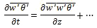 (31)
(31)Describing turbulence in the boundary layer involves more unknowns than prognostic equations, a classic problem in meteorology, and geophysical fluid dynamics in general, referred to as the closure problem.
How is the problem solved? One solution is to approximate the unknown variables in terms of the known variables using various orders of closure. These closure assumptions are categorized by their statistical order and how much non-localness is included. Figure 6F1.1 depicts local and non-local closure assumptions during one time step.
A first order closure keeps 1st and 2nd order terms, which include the following types of variables:
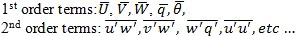
The order is named for the highest order forecast equation, so a first order closure includes only (11). A second order closure would retain equations (11) and (31). Parameterizations of the ABL use different closure assumptions. The choice of closure depends on the environment and phenomena being predicted.
Focus 1: Modeling the Tropical Boundary Layer »
6F1.2 Parameterization
The primitive equations used to describe the large-scale evolution of the atmosphere (Chapter 9, Section 9.4.1.1Chapter 9, Section 9.4.1.1) do not account for the small-scale interactions in the ABL, which are totally sub-grid scale; therefore ABL motions and processes need to be parameterized.
ABL parameterizations or schemes determine the vertical fluxes of temperature, moisture, and momentum, and, hence, their contribution to the time evolution of the ABL and ultimately the ABL contribution to tropical convection. The surface fluxes transferred to the atmosphere are affected by the choice of other parameterizations, including land surface, hydrology, radiation field, surface layer physics, and cloud field.
The uncertainties in model representation of the marine boundary layer are connected with: (i) Parameterization of turbulence and shallow convection, (ii) Algorithms used for wind-wave coupling, and (iii) Scarcity of real-time ocean data model initialization. A land surface model provides heat and moisture fluxes over land points; it updates the lands state variables, include the ground (skin) temperature, soil temperature profile, soil moisture profile, snow cover, and possibly canopy properties.
Focus 1: Modeling the Tropical Boundary Layer »
6F1.2 Parameterization »
6F1.2.1 Mixing Parameterization
The Mellow-Yamada-Janjic (MYJ) and Yonsei University (YSU) schemes are two of the most commonly-used ABL mixing parameterization schemes. They have different assumptions about mixing at the top of the BL (Fig. 6F1.2), which can produce markedly differences in forecasts.
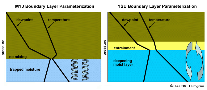
MYJ scheme
- Assumes that no mixing occurs with air above the ABL, while air in the ABL is mixed intensely among adjacent layers
- Related effects:
- Too much low-level moisture
- Not enough dry air is entrained into the ABL from above
- Additionally, a stratocumulus deck may form or fail to erode, further limiting daytime temperatures and CBL heights
YSU scheme
- Assumes deep mixing extends to the layer above the current ABL top (non-local mixing)
- Related effects:
- The boundary layer grows and moisture is carried through too deep of a layer
- The capping inversion erodes too much
- Low clouds and cold air damming are prematurely eroded
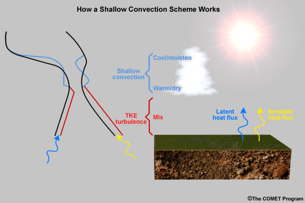
The entrainment zone or transition layer is parameterized using a shallow convection scheme (Fig. 6F1.3). Such schemes can be extensions of the ABL scheme or separate. They account for the upward mixing of moisture and heat, and the downward mixing, of heat and momentum, between the model ABL and the free atmosphere. Shallow convection schemes are also needed in non-hydrostatic models that explicitly predict convection (without cumulus parameterization).
Focus 1: Modeling the Tropical Boundary Layer »
6F1.3 Types of Boundary Layer Models
Focus 1: Modeling the Tropical Boundary Layer »
6F1.3 Types of Boundary Layer Models »
6F1.3.1 Mixed Layer or Slab Models
Many of the early (1970s and 1980s) simulations of the boundary layer used mixed layer models, often called slab, bulk, or integral models, which model just ensemble statistics using Reynolds averaging. Figure 6F1.4 shows an example of a mixed layer model that uses a local, first order closure.

This method is suitable where vertical gradients are small or where it is adequate to use vertically-averaged quantities, and where entrainment and growth of the mixed layer are of particular interest. The boundary layer height is calculated separately and the top of the BL is treated as a surface. It is efficient for modeling a mixed layer that is capped by a strong inversion and in accounting for mixed layer-cloud instability and interactions between the ABL and cumulus clouds. These advantages make it appropriate for modeling the trade wind regime. This approach is less adaptable to situations where the transition to the free atmosphere is more gradual. High resolution, 3-D models have mostly replaced this type of model.
Focus 1: Modeling the Tropical Boundary Layer »
6F1.3 Types of Boundary Layer Models »
6F1.3.2 Direct Numerical Simulation
Direct numerical simulation (DNS) resolves all relevant scales of motion so that no parameterization is needed.151,158 The Navier Stokes equation of motion for incompressible flow helps to illustrate the immense challenges of DNS of turbulent motion in the atmosphere:
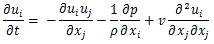 (32)
(32)where ui is velocity, p is pressure, ρ is density, and v is the molecular kinematic viscosity (assumed constant). This equation applies to all scales, from planetary waves (order 107 m) to dissipative eddies (order of 10-4 m). However, to resolve all motion in the convective boundary layer would require a grid spacing of 1 mm, which is beyond current and foreseeable computing capability for simulating the atmospheric BL. Studies using DNS of turbulent velocity field have been limited to flow with large Reynolds number, Re=1000, which is much smaller than the Re =106 108 found in the atmosphere.159 Given the futility of directly simulating turbulent flow in the ABL or in moist convection, alternative methods are needed.
Focus 1: Modeling the Tropical Boundary Layer »
6F1.3 Types of Boundary Layer Models »
6F1.3.3 Large Eddy Simulation
Large eddy simulation (LES) is a tool for diagnosing and predicting turbulent flows that was first applied to the atmospheric boundary layer in the early 1970s.88,160,161 It is an intermediate approach between the mixed layer models and direct numerical simulation. LES resolves large eddies, which are most important for turbulent energy, momentum, and other transport in the boundary layer (Section 6.3.6Section 6.3.6) and filters out the sub-grid scale (Fig. 6F1.5).
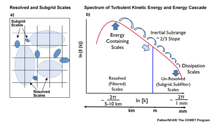
Large eddy energy and other fluxes are calculated explicitly while small eddies, which have small energy and fluxes, are parameterized. The effect of the small eddies on the resolved scale are modeled with a sub-filter scale (SFS) stress model.162 The LES is supposed to be independent of the SFS model.
LES use has increased in correspondence with advances in high-performance computing, model architecture, and grid-nesting formulations. Fig. 6F1.6 shows how an LES was used to simulate tropical boundary layer cellular convection and the related aerosol interactions. LES simulations of deep tropical convection have found that the tri-modal vertical distribution of clouds (Fig. 5.15) could only be reproduced with vertical grid spacing of 50-100 m in the mid-to-low troposphere.163
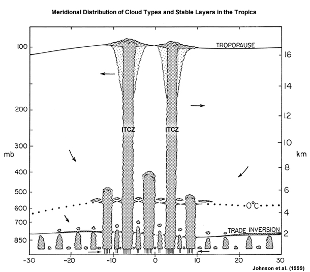
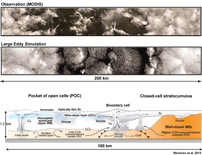
LES can be coupled with mesoscale models as illustrated in Fig. 6F1.7, where the LES provides explicit values for surface and ABL variables at the mesoscale model grid points. There are challenges to coupling an LES with realistic ABLs, such as how to specify the inflow boundary conditions, uncertainties in how to represent the sub-filtered scales near irregular boundaries, and the proper scaling so that the ensemble statistics are represented.
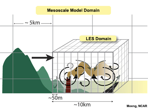
For simulating deep moist convection, which is ubiquitous in the humid tropics, the grid resolution for the LES should be guided by the intended use of the model output. A grid-size on the order of 100 m is recommended in order to adequately represent the turbulent kinetic energy151 and fluxes associated with moist convection.
Operational Focus
Vertical structure of the tropical troposphere
- Profiles of temperature and humidity in the tropicsProfiles of temperature and humidity in the tropics
- The tropical boundary layerThe tropical boundary layer
- Identify the top of the mixed layerIdentify the top of the mixed layer
- The Trade Wind Inversion and its impact on cloud developmentThe Trade Wind Inversion and its impact on cloud development
Buoyancy and static stability
- Criteria for unstable, stable, and neutral environmentsCriteria for unstable, stable, and neutral environments
Turbulence
- Criteria for turbulent flowCriteria for turbulent flow
- Typical wind profiles in the tropical marine boundary layerTypical wind profiles in the tropical marine boundary layer
Air pollution and aerosol transport
- Mixed layer depth estimationMixed layer depth estimation
- Dispersal in the tropical marine boundary layerDispersal in the tropical marine boundary layer
- East-to-west profile of CCN concentration in trade wind regimeEast-to-west profile of CCN concentration in trade wind regime
- Dust transportDust transport
- Sea-breeze effects on air pollutionSea-breeze effects on air pollution
- Smoke transportSmoke transport
Surface heat fluxes
- Global and seasonal distribution of surface latent and sensible heat fluxesGlobal and seasonal distribution of surface latent and sensible heat fluxes
Diurnal cycle of the boundary layer
- Convective, stable, residual, and neutral boundary layersConvective, stable, residual, and neutral boundary layers
- Differences between boundary layer over ocean and landDifferences between boundary layer over ocean and land
- Nocturnal low-level jetNocturnal low-level jet
- Differences between dry and humid tropicsDifferences between dry and humid tropics
Sub-cloud environment and cloud development
- Cloud patterns with cold air outbreak over warm oceanCloud patterns with cold air outbreak over warm ocean
- Thermodynamic environment and impact on cloud growthThermodynamic environment and impact on cloud growth
- Air-sea temperature difference and wind speed effect on cloud patternAir-sea temperature difference and wind speed effect on cloud pattern
- Small island and formation of wake convergence cloudsSmall island and formation of wake convergence clouds
Cumulus convection
- Growth of ordinary cumulus in fair weatherGrowth of ordinary cumulus in fair weather
- Evolution of tropical mesoscale disturbanceEvolution of tropical mesoscale disturbance
- Stabilization of the boundary layer by deep convectionStabilization of the boundary layer by deep convection
Numerical weather prediction
- Rationale for cumulus parameterizationRationale for cumulus parameterization
- Learn how clouds and their effects are represented in modelsLearn how clouds and their effects are represented in models
- Advantages and limitations of cumulus parameterizationAdvantages and limitations of cumulus parameterization
- Advantages and limitations of cloud-system resolving modelsAdvantages and limitations of cloud-system resolving models
- Advantages and limitations of different boundary layer schemesAdvantages and limitations of different boundary layer schemes
Summary
The chapter provided qualitative and quantitative information about energy and momentum transport from the surface through the troposphere, over a range of time scales. Understanding vertical transport is important because tall cumulus in the tropics provide the upward heat transport that balances radiative cooling and poleward export at the top of the troposphere. In order for models to be able to represent vertical transport, its associated processes need to be identified and their respective contributions and/or effects quantified. Some basic methods of representing convection and its effects in regional and global models were explored; including cumulus parameterization, cloud-system resolving models, and super-parameterization. Additionally, the vertical transport of chemical constituents and aerosols, critical for air quality, radiative balance, and climate, were examined.
Deep cumulus convection is the primary means of heat, moisture, momentum and chemical transport in the tropics. Transport from the surface to the tropopause can happen within hours in deep cumulus convection, which occupy only small areas of the tropics. For most of the tropics, the time scale of overturning between the surface and the troposphere occurs over weeks to a month.
Vertical heat and moisture distributions vary according to the convective modes and how energy is partitioned between condensation, evaporation, precipitation, sensible heat, and radiative cooling. Diabatic heating rates peak in the upper troposphere in organized deep convection, in contrast to shallow cumulus, in which heating rates are smaller, peak in the lower troposphere, and are near zero above the inversion. Large-scale tropical circulations such as the Walker and Hadley circulations result from vertical motion that is a response to the spatial distribution of vertically integrated net heating, with the maximum diabatic heating due latent heat release in deep convection.
The peak heating rate shifts higher in the troposphere as the stratiform portion of organized convection increases. Additionally, organized deep convection in the free troposphere stabilizes the sub-cloud layer, inhibiting convection until the mixed layer is restored to its neutrally stable undisturbed state. Vertical momentum flux transport in mesoscale convective systems is significantly different from transport in fair weather or dis-aggregated convection. Generally, in the lowest layers, where friction dominates, surface energy is transported upward while momentum is mixed downward as wind decrease to zero at the surface interface. However, in tropical mesoscale convective systems, vertical momentum flux is transported upgradient with flow perpendicular to a convective line that is tilted rearward.
The first layer of exchange is the surface interface, where the ocean has less friction, smaller diurnal temperature range, and lower roughness height than land. Latent heat flux is the primary means of surface to air transport in the global annual mean. Its maximum values occur over warm, western boundary currents and its minima over eastern tropical oceans. Turbulent surface fluxes of latent heat, sensible heat, and momentum are determined using Reynolds averaging of temperature, specific humidity, and momentum and the differences between those bulk variables at sea surface and at a given height above the surface. Transport from the surface continues upward through the atmospheric boundary layer, which has a fast response to changes at the surface and is marked by friction and turbulence. Turbulence is created by buoyancy and shear. The surface layer, which is mainly super-adiabatic is the root of thermals generated by surface heating. During daytime, large turbulent eddies transport latent heat, sensible heat, and momentum, through the rapidly expanding mixed layer, which occupies most of the convective boundary layer. Large eddies in the CBL have an overturning time of the order of 15 minutes. At night, the surface cools, the lower troposphere becomes stably stratified, and a stable boundary layer develops. At the top of that stable layer, winds accelerate with the loss of friction, creating a nocturnal low-level jet. The low-level jet can contribute to vertical transport by generating shear-induced turbulence and acting as a conduit for warm, moist air for deep convection.
Vertical heat and moisture transport in the fair-weather marine boundary layer, which is much shallower and less variable in depth than land, depends on the presence or absence of clouds. With clouds, sensible heat flux convergence in the shallow marine boundary layer is sufficient to offset the heat lost to radiative cooling. Boundary layer clouds have their roots in the sub-cloud layer whose properties help to determine whether horizontal rolls or cells will form. Stratocumulus and boundary layer cumulus occupy large areas of the tropics but their role in vertical transport is secondary to tall cumulus in the free troposphere. They have long-term impact on the radiation budget and climate. Shallow cloud processes, which help to maintain the trade wind inversion, are a challenge for numerical models. Shallow cumuli are capped by the inversion, which weakens and slopes upward towards the west and the equator. The inversion is maintained by subsidence and divergence away from the subtropical anticyclones and by sensible heat flux over the eastern tropical oceans. With warmer SSTs to the west, decreasing divergence, and more instability, the inversion weakens.
A focus section on the tropical boundary layer modeling summarizes methods for representing turbulent energy and momentum fluxes and convection in this critical layer that feeds atmospheric convection, which in turn drives tropospheric circulations.
Questions for Review
- Describe the vertical structure of the tropical troposphere and time scales of vertical transport through its layers.
- Describe the general distribution of vertically integrated heating in the tropics and how that distribution is related to tropical circulations.
- Explain how turbulence is generated and how it contributes to vertical transport.
- Describe why the mixed layer properties are important to the dispersal of smog and low-level pollutants.
- Discuss the processes of exchange between the surface and the atmosphere for sensible heat, latent heat, and momentum in fair weather conditions.
- Describe the processes that contribute to the growth of tropical cumulus.
- Explain how and why the vertical transport of horizontal momentum in organized deep convection differs from transport in the undisturbed boundary layer.
- Compare and contrast the vertical transport of energy in shallow cumulus, deep convection, and mesoscale stratiform clouds.
- Explain how convective updrafts and downdrafts contribute to vertical transport of energy and mass flux in tropical cumulus.
- Describe how the marine boundary layer interacts with land surfaces to disperse pollutants in the lower troposphere.
- Describe some mechanisms by which the trade wind stratocumulus layer is maintained.
- How do the subtropical anticyclones contribute to the vertical transport of heat and moisture?
- Describe at least one process that helps to maintain the trade wind inversion.
- List the layers of the tropical boundary layer and describe the vertical transport processes in each.
- What are the major differences between the tropical marine and continental boundary layers?
- Describe the primary objective and limitations of cumulus parameterization schemes.
- Compare and contrast the vertical distribution of the apparent heat source for fair weather cumulus, mature tropical mesoscale convective system (MCS), and decaying MCS.
- Describe the strengths and limitations of cloud resolving models.
- Explain the impacts of vegetation removal on the Bowen ratio, vertical transport, and climate.
- Describe three important surface-to-atmosphere interface processes for land and ocean, respectively.
- Compare and contrast the convective and stable boundary layers, including their evolution during the diurnal cycle and impact on vertical transport.
- Describe how trace gases and aerosols are transported by the marine boundary layer and tropical clouds.
- Explain how the morphology of shallow cumulus is influenced by sub-cloud properties.
- Describe how cumulus processes and effects are generally represented in regional and global numerical models.
Brief Biographies
Alan Betts
Alan Betts performed important early work in tropical convection during the GATE experiment. Raised in the United Kingdom, Alan Betts obtained a B.A. and an M.A. in natural sciences from the University of Cambridge and a Ph.D. in Meteorology from Imperial College, University of London in 1970. He accepted a post-doctoral position at the Atmospheric Science Department of Colorado State University from 1970-1971 and then served as assistant and associate professor there from 1971-1979. During that time, he was appointed the Convection Subprogram Scientist for the GATE experiment – an attempt to understand cumulus convection in the tropical atmosphere and its role in general circulation. He next moved to Vermont and founded the company Atmospheric Research, whose mission is to understand Earths climate, develop better Earth-system models, and help society better understand the challenges of global climate change. He has studied climate in the Konza Prairie in Kansas, the boreal forest of Canada, and a forest in the Brazilian Amazon. Betts is a fellow of the American Meteorological Society, Royal Meteorological Society, and the American Association for the Advancement of Science. In 1977 he won a Special Award from the American Meteorological Society along with Stephen K. Cox and Edward J. Zipser for outstanding contributions and leadership in the conception, documentation, and execution of the scientific aircraft program of the GARP Atlantic Tropical Experiment. He won the AMSs Jule G. Charney Award in 2007 for pioneering and sustained contributions to the understanding of the atmospheric boundary layer, cumulus convection, and land-surface-atmosphere interactions.
Michael (Mike) Garstang
Mike Garstang, Professor Emeritus at the University of Virginia in the Department of Environmental Sciences, conducted important early work in tropical marine and continental meteorology, convective storms, trace gas and aerosol transport, and experimental meteorology. Garstang was born in South Africa and moved to the United States in the late 1950s. He received B.A. and M.A. degrees in geography from the University of Natal and M.S. and Ph.D. degrees in meteorology from Florida State, the latter in 1964. He was named a professor at the University of Virginia in 1971. During his scientific career, he helped design and carry out many large experiments including BOMEX, GATE, and ABLE. In his work with the GATE experiment, he studied moist convection in mesoscale and smaller phenomena. Garstang has also studied atmospheric controls on elephant calls over long distances at low frequencies in Namibia. He has also taken an interest in the science of weather modification and has testified before the United States Senate on the subject.
Michio Yanai
Michio Yanai made important contributions to tropical meteorology , including work on mixed Rossby-gravity wave (also called the Yanai wave), on the effect of the Tibetan Plateau on the Asian Monsoon, and a foundational 1964 review paper on how tropical cyclones form that served as the gold standard on the topic for more than 10 years. Dr. Yanai spent his childhood in Chigasaki, Japan. He earned a D. Sc. In geophysics from the University of Tokyo in 1961 and served as assistant professor there from 1965-1970. In 1970, he was named a professor at the University of California at Los Angeles. For 14 years, he published the UCLA Tropical Meteorology and Climate Newsletter. In addition to his other work on tropical meteorology, he is also remembered for a systematic method of estimating apparent heat sources and moisture sinks and correlating them with properties of convective systems. In 1986 he won the Jule G. Charney Award for highly original contributions to enlarging our knowledge of the dynamics of the atmosphere, particularly in the tropics, and in 1993 he received the Fujiwara Award from the Meteorological Society of Japan. Dr. Yanai died in 2010 at the age of 76.