About the Lesson
This lesson introduces you to three of the four near-infrared imager bands on the GOES R-U ABI (Advanced Baseline Imager), focusing on their spectral characteristics and how they affect what each band observes. Discussion of the 0.86 micrometer or "veggie" near-IR band is not included here. Because of its similarity to the visible bands, information on the "veggie" band appears in the Visible and Near-Infrared Bands lesson.
On completing the lesson, you should be able to:
- Identify the ABI's three near-infrared spectral bands (not including the 0.86 micrometer "veggie" band) and various phenomena that can be detected in the spectral regions they cover
- Identify which of the near-IR bands is most sensitive to atmospheric absorption and describe the implications for observing clouds and surface features
- Identify sun glint in near-IR imagery
Please note that this lesson was originally published prior to the launch of GOES-16 and used imagery from the Himawari-8 geostationary satellite to illustrate GOES-R ABI capabilities. The Himawari-8 imager, the AHI (Advanced Himawari Imager), has bands nearly identical to the ABI on board the GOES R-U series. In the interest of time, some of the original Himawari-8 imagery is still included where geographical context is not critical for understanding the concept.
Introduction
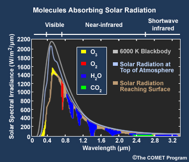
The Advanced Baseline Imager's (ABI) near-infrared bands are in the region of the electromagnetic spectrum where the sun emits about 52% of its energy from 0.7 to 2.5 micrometers. Incoming solar energy is scattered and absorbed by molecules, clouds, and aerosols, with the amount of attenuation varying with wavelength.
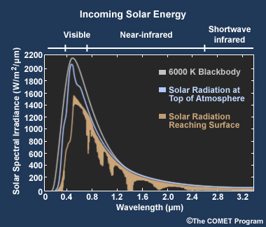
While most visible energy is not absorbed by Earth's atmosphere, more than half of near-infrared energy is absorbed in the troposphere, mostly by water vapor, other trace gases, and darker aerosols like soot, ash, and dust when they contain significant amounts of carbon or carbon residue.
Clouds and surface features also reflect near-IR energy as they do visible energy. Clouds however, exhibit much greater variability in reflection as a function of cloud phase (water vs. ice) and particle size.
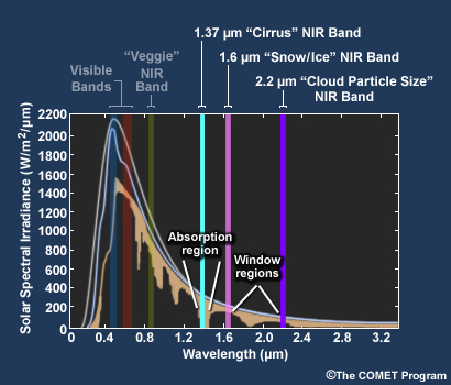
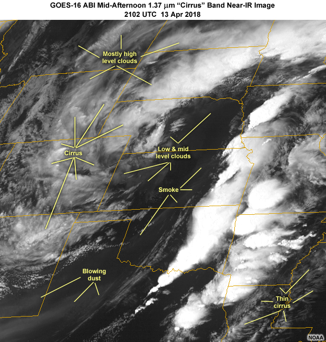
The first of the three bands we'll explore is located at 1.37 micrometers and known as the "cirrus" band. Energy in this band is strongly absorbed by tropospheric water vapor. This blocks energy from land and low to mid-level atmospheric features and allows higher level cloud tops and cirrus clouds to stand out. The strong water vapor sensitivity also enables detection of very thin cirrus often missed by visible and other infrared imaging bands.
The second of the three bands is located at 1.6 micrometers and known as the "snow/ice" band. It lies within an atmospheric window region where there is little absorption by gases.
And the third band, located at 2.2 micrometers and known as the "cloud particle size" band, is also located within an atmospheric window region. Given that little atmospheric absorption is present in both 1.6 and 2.2 micrometer bands, they are well-suited for characterizing surface and cloud features.
ABI Near-IR Bands: Land and Water
This graph shows reflectances for clouds and a variety of different surface types. Since the 1.37 micrometer "cirrus" band is strongly influenced by water vapor attenuation and does not see most surfaces and lower tropospheric cloud cover, this page will focus on the 1.6 and 2.2 micrometer bands, both located in atmospheric window regions of the near-IR spectrum.
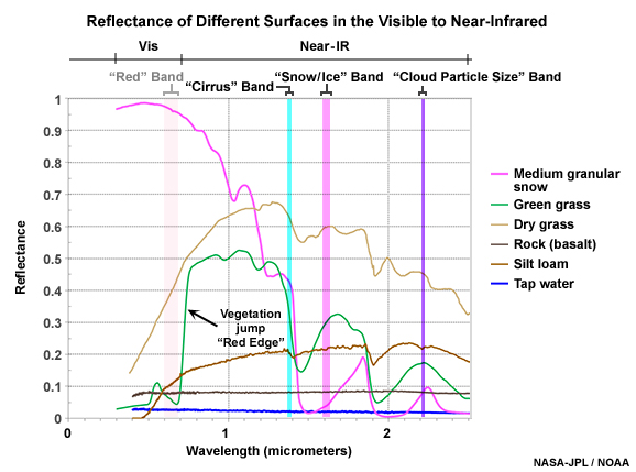
Referring to the plot, for most surface objects especially those containing water or ice (vegetation, wet soil, snow and ice cover for example) there is an overall trend of decreasing reflection with wavelength. Most of this is the result of an increase in absorption by water toward longer near-IR wavelengths. The relatively deep valleys in some of the reflection curves indicate where absorption by water (liquid and frozen) in a material is particularly strong.
In contrast to "wet" objects on land, we see that reflectances for bare dry soil and rocky surfaces remain relatively constant. Water surfaces (lakes, rivers, oceans) are poorly reflective, with almost no reflection beyond 0.9 micrometers.
While thick cloud cover remains relatively reflective in the near-IR, snow cover (lower magenta curve) becomes poorly reflective which has implications for discriminating clouds vs. snow cover. The effect is not as pronounced for ice clouds, but they also become less reflective than liquid water clouds which has implications for determining cloud-top phase.
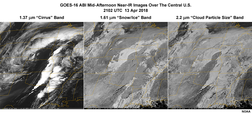
The example below compares near-IR bands from GOES-16's ABI imager. The GOES-16 0.64 "red" band is included for comparison because of it's familiarity to users as the 0.63 micrometer visible band on the legacy GOES satellites.
Notice the distinct darkening of ice cloud tops especially in the 1.6 micrometer image, whereas water clouds and land surfaces are relatively bright. This reflectivity difference in clouds is what helps determine cloud-top microphysical properties used for defining cloud type and in the case of convection inferring cloud maturity and convective strength.
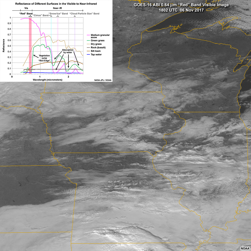
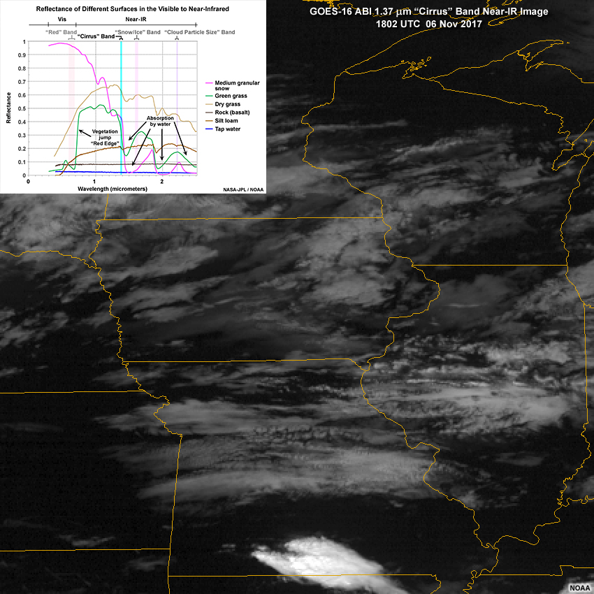
Note: In the 1.37 µm "cirrus" band, surface and lower-level features (land, oceans, cloud cover, etc.) appear relatively dark due to strong absorption of solar energy by atmospheric water vapor in the 1.3 to 1.5 µm near-IR region.
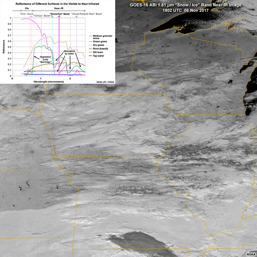
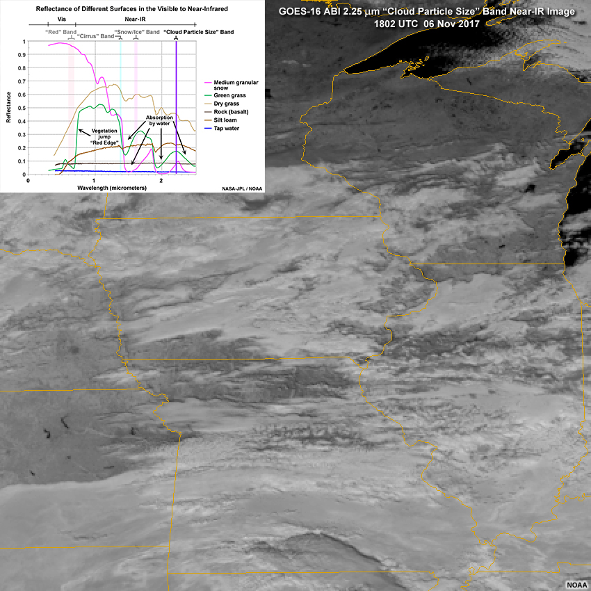
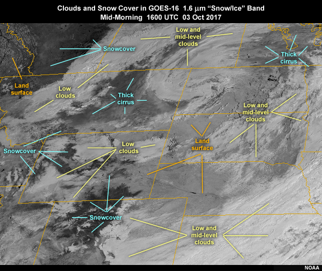
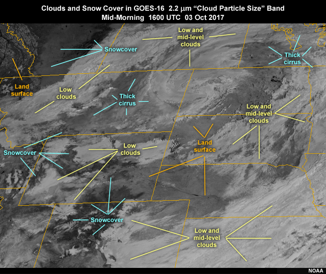
The second example (below) shows a fall season storm system as it spreads a variety of weather across the central U.S. and southern Canada. The focus is on the 1.61 "snow/ice" and 2.2 "cloud particle size" bands, and comparing a variety of different cloud and surface types including snow cover.
As in the previous example, the darker less reflective ice cloud tops stand out in contrast to the brighter more reflective water clouds and land surfaces.
We also see darker features over portions of the Rocky Mountains and Southern Alberta. These are indicative of how these two bands observe snow cover's poorly reflective near-IR properties. Some of the relatively bright patches appearing between snow covered areas are actually bare ground. And since there is less live vegetation at this time of year, most land surfaces appear even more reflective than they would during the growing season.
Below are animations for the same example. We see that the combination of varying reflectance and image looping gives geostationary satellites a distinct advantage for distinguishing between surface features and more rapidly evolving cloud cover.
Below is a daytime Red-Green-Blue (RGB) color composite image made from one visible band and two near-IR bands for the same scene. It consolidates the information from each of the three bands into a single product that provides more information on different surface and cloud features than a single image can provide. RGB imagery is covered in more depth in the SatFC-G Multi-Channel Interpretation Approaches lesson.
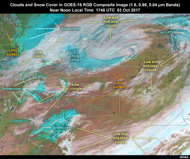
In this false-color RGB composite image, ABI's 1.61 µm snow/ice band is assigned to red, the 0.86 µm veggie band to green, and the 0.64 µm red band to blue. In the NWS AWIPS display system, this product is also known as the Day Land Cover RGB.
ABI Near-IR Bands: Clouds
The ABI's near-IR bands bring a new cloud detection capability to geostationary satellite coverage over the Western Hemisphere. While the 1.37 micrometer "cirrus" band highlights high clouds and very thin cirrus, the 1.6 and 2.2 micrometer bands take advantage of a relatively large difference between the reflected energy components of water and ice cloud particles.
Recall from the previous discussion that due to strong absorption of solar energy by water vapor at 1.37 micrometers, lower-level features in the "cirrus" band appear dark or undistinguishable compared to higher level cirrus and convective cloud tops. And since the 1.6 and 2.2 micrometer bands are in atmospheric "window" regions, we readily see Earth's surface and most cloud cover regardless of altitude.
For a more direct comparison of the three near-IR images, drag the slider under the larger version of the image shown below.
Drag the slider to compare the three ABI Near-IR images.
Note: The second image shows the 1.37 µm "cirrus" band with GLM lightning "Group" data points (parallax corrected) over a 5-minute period ending at the time of the image. This helps identify cloud tops associated with deep convection. A GLM "Group" consists of one or more simultaneous GLM optical detections (or "Events", sampled every 2 milliseconds) observed in adjacent pixels.
The 1.6 and 2.2 micrometer bands are not only useful for distinguishing between water and ice cloud phases, they detect variations in reflected solar energy that result from changes in cloud particle size near cloud top. This information is leveraged to make derived products for characterizing cloud-top microphysical properties. The products can provide valuable insight into cloud evolution, and for deep convection, help assess the potential severity of developing thunderstorms.
A number of features and trends in cloud-top reflectance to look for when viewing daytime 1.6 and 2.2 micrometer imagery include:
- Water clouds are more reflective than ice clouds
- The thicker the water and ice cloud, the more reflective it becomes
- Cloud reflectance increases as cloud particle size becomes smaller (for both water and ice clouds)
The animation below highlights the 1.6 "snow/ice" band as it shows developing thunderstorms that produced large hail and damaging winds over the central and southern High Plains of the U.S. on the afternoon and evening of August 10, 2017. The 0.64 micrometer "red" visible band (on the left) is shown for comparison. Notice in the "snow/ice" band how cloud tops turn darker shades of grey as glaciation occurs in the towering cumulus. Furthermore, different shades of grey indicate different ice particle sizes at cloud top, with brighter grey shaded areas indicating smaller ice particles.
ABI Near-IR Bands: Hot Spots
Another interesting aspect of the 1.37, 1.6 and 2.2 micrometer bands is their sensitivity to hot spots, especially noticeable during nighttime when clouds and surfaces are not illuminated by incoming solar energy. The 2.2 micrometer band has greater sensitivity since it's closer to the maximum emitting temperature of an actively burning fire. Notice in the plot below that the energy from a fire increases more at 2.2 than at 1.37 and 1.6 micrometers. We need to remember that in the 1.37 micrometer "cirrus" band, surface features are largely blocked from view due to the atmosphere's strong water vapor absorption from 1.3 to 1.5 micrometers.
For cooler hot spots, longer wavelengths in the shortwave IR region become more effective for characterizing heat sources. This is also where the ABI's 3.9 micrometer IR band is located, which is covered in the IR Bands lesson.
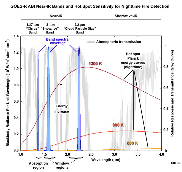
Note: The light grey curve shows atmospheric near-IR transmittance as a function of wavelength. The greater the transmittance, the less absorption of energy by gases and therefore the more energy that's allowed to pass through the atmosphere. The 1.37 µm “cirrus” band experiences strong absorption by water vapor (shown as a valley in the transmittance curve), so the transmittance is very weak and mostly upper tropospheric features are seen, e.g. cirrus, convective cloud tops, high-level dust and volcanic ash.
The animation below shows 1.6, 2.2 and 3.9 micrometer images during the first 12 hours of several wildfires in northern California. Fanned by 50 mile per hour winds, the fires grew rapidly and consumed 80,000 acres in just 18 hours on the 8th and 9th of October 2017. The 3.9 micrometer "shortwave window" IR band is included for comparison and because of its familiarity to most users of GOES and polar-orbiting satellite imagery for detecting hot spots. In conjunction with the 3.9 shortwave window and other IR bands, ABI's near-IR detection capabilities allow for significant improvements in fire detection and monitoring.
Notice that because the animation begins a couple hours after sunset, the fires' infrared emissions are clearly seen in all three bands. As the loop enters the daytime hours however, the added solar energy approaches the near-IR emissions of the fires. The result, the 1.6 and 2.2 micrometer bands no longer distinguish the fires from the surrounding land as well as they did during nighttime.
Sun Glint Over Water
As in the visible, sun glint is an important phenomenon that must be considered when viewing near-IR images over water. When water surfaces are smooth, large reflections occur when the sun and satellite are properly aligned. In the two loops, notice the bright region that moves from east to west as the sun moves. We also see patches of relatively bright or dark within the larger glint pattern. Some patches change from relatively dark to bright as the sun's reflection approaches, and then back to dark again, whereas other areas remain relatively dark farther away from the center of the glint pattern. These patches are all indicative of relatively calm waters surrounded by a rougher sea surface.
Sun glint may reveal other interesting surface features. Much like wind induced changes in surface roughness, water currents, internal waves, and changes in surface tension caused by oils or surfactants, alter the reflective properties of a water surface which can be highlighted by sun glint.
Summary
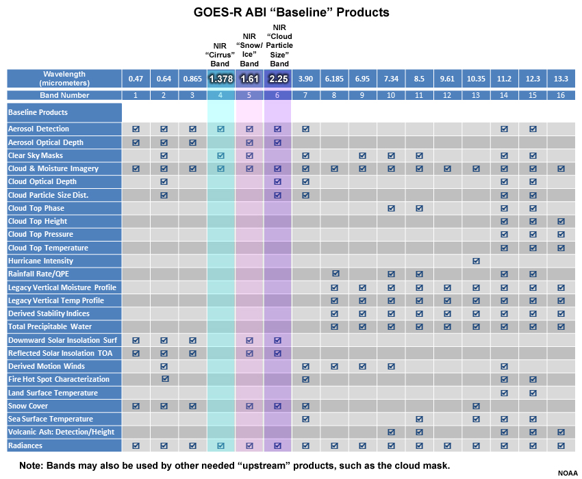
The ABI's near-IR bands provide forecasters with high spatial and temporal resolution imagery and products for monitoring a variety of surface and atmospheric phenomena, some of which were highlighted in this lesson. In addition to imagery, near-IR bands contribute to a host of "baseline" derived products for monitoring aerosols, clouds, radiation and snow cover. Based on scientific algorithms, these products provide quantitative data on various physical properties by extracting information from different band groupings known to be sensitive to a particular property.
Visible and Near-IR Band Characteristics:
- Spectral Coverage
- "Cirrus" band: 1.37 μm central wavelength, 1.37 – 1.38 μm (GOES-R ABI), Near-Infrared
- "Snow/ice" band: 1.6 μm central wavelength, 1.59 – 1.63 μm (GOES-R ABI), Near-Infrared
- "Cloud particle size" band: 2.2 μm central wavelength, 2.22 – 2.27 μm (GOES-R ABI), Near-Infrared
- Resolution (at satellite sub-point)
- "Cirrus" band: 2-km field of view
- "Snow/ice" band: 1-km field of view (to match the high resolution of the visible bands and "veggie" band for better inter-band comparisons; to facilitate derived products and image combinations, Red-Green-Blue (RGB) color composites for example)
- "Cloud particle size" band: 2-km field of view
- Quality Improvements
- Low noise and improved pixel geolocation and registration (frame to frame pixel stability)
Application Considerations:
- "Cirrus" Band
- Daytime only for cloud applications
- Sees scattered and reflected energy (mainly in the upper troposphere)
- Sees mainly upper tropospheric cloud tops
- Very sensitive to thin cirrus
- May see high-level dust and ash
- "Snow/Ice" and "Cloud Particle Size" Bands
- Daytime only for snow cover and cloud applications
- Bands are sensitive to cloud-top microphysics (phase and particle size)
- "Snow/ice" band is more sensitive to water vs. ice differences (cloud phase and ground features)
- "Cloud particle size" band is more sensitive to cloud particle size differences
- Nighttime for fire and hot spot applications
- Optimal use may require multi-band image combinations in the form of derived products (as shown in the table) and RGB imagery
- Daytime only for snow cover and cloud applications
You have reached the end of the lesson. Please complete the quiz and share your feedback with us via the user survey.
Resources
Internet Resources
- Official GOES-R Program Site, http://www.goes-r.gov/
- GOES-R Training Overview, http://www.goes-r.gov/users/training.html
- GOES-R: Benefits of Next-Generation Environmental Monitoring, http://www.meted.ucar.edu/training_module.php?id=509
- GOES-R Proving Ground Page, http://www.goes-r.gov/users/proving-ground.html
- GOES-R Documentation Page, http://www.goes-r.gov/resources/docs.html
- GOES-R Scientific Publications, http://www.goes-r.gov/resources/Scipubs/index.html
- GOES and POES Conferences and Meetings, http://www.goes-r.gov/users/conf-mtgs.html
- UW CIMSS Satellite blog and GOES-R, http://cimss.ssec.wisc.edu/goes/blog/archives/category/goes-r
- VISIT: SHyMet for Forecasters: GOES-R 101 Training Session, http://rammb.cira.colostate.edu/training/shymet/forecaster_goesr101.asp
Advanced Baseline Imager (ABI) Specific
- GOES-R ABI Instrument Page, http://www.goes-r.gov/spacesegment/abi.html
- GOES-R ABI: Next Generation Satellite Imaging, http://www.meted.ucar.edu/training_module.php?id=987
- ABI Fact Sheet, http://www.goes-r.gov/education/docs/Factsheet_ABI.pdf
- ABI Bands Quick Information Guides, http://www.goes-r.gov/education/ABI-bands-quick-info.html
References
GOES-R
- Schmit, T., P. Griffith, M. Gunshor, J. Daniels, S. Goodman, and W. Lebair, 2017: A closer look at the ABI on the GOES-R series. Bull. Amer. Meteor. Soc., 98, 681-698, doi: https://doi.org/10.1175/BAMS-D-15-00230.1.
- Schmit, T.J., S.S. Lindstrom, J.J. Gerth, and M.M. Gunshor, 2018: Applications of the 16 spectral bands on the Advanced Baseline Imager (ABI). J. Operational Meteor., 6, 33-46, doi: https://doi.org/10.15191/nwajom.2018.0604.
- Additional GOES-R and GOES Related Scientific Publications and other documentation (available on the GOES-R Program Site):
Publications: http://www.goes-r.gov/resources/Scipubs/index.html
Documentation: http://www.goes-r.gov/resources/docs.html
Contributors
COMET Sponsors
MetEd and the COMET® Program are a part of the University Corporation for Atmospheric Research's (UCAR's) Community Programs (UCP) and are sponsored by
- NOAA's National Weather Service (NWS)
with additional funding by: - Bureau of Meteorology of Australia (BoM)
- Bureau of Reclamation, United States Department of the Interior
- European Organisation for the Exploitation of Meteorological Satellites (EUMETSAT)
- Meteorological Service of Canada (MSC)
- NOAA's National Environmental Satellite, Data and Information Service (NESDIS)
- NOAA's National Geodetic Survey (NGS)
- National Science Foundation (NSF)
- Naval Meteorology and Oceanography Command (NMOC)
- U.S. Army Corps of Engineers (USACE)
To learn more about us, please visit the COMET website.
Project Contributors
Program Managers
- Wendy Abshire – UCAR/COMET
- Bruce Muller – UCAR/COMET
Project Lead and Meteorologist
- Patrick Dills — UCAR/COMET
Instructional Design
- Bruce Muller — UCAR/COMET
Science Advisors and Contributors
- Dr. Jordan Gerth — Cooperative Institute for Meteorological Satellite Studies (CIMSS)/NOAA/University of Wisconsin
- Tim Schmit — NOAA NESDIS STAR/ASPB @ CIMSS
Graphics/Animations
- Steve Deyo — UCAR/COMET
Multimedia Authoring/Interface Design
- Gary Pacheco — UCAR/COMET
Audio/Video Editing/Production
- Steve Deyo – UCAR/COMET
Audio Narration
- Vanessa Vincente — UCAR/COMET
GOES-16 Imagery Provided By
- NOAA
Himawari-8 Imagery Provided By
- SSEC/Unidata Community ADDE Open Archive – University of Wisconsin, Madison
- Japan Meteorological Agency (JMA)
COMET Staff, August 2018
Director's Office
- Dr. Elizabeth Mulvihill Page, Director
- Tim Alberta, Assistant Director Operations and IT
- Paul Kucera, Assistant Director International Programs
Business Administration
- Lorrie Alberta, Administrator
- Auliya McCauley-Hartner, Administrative Assistant
- Tara Torres, Program Coordinator
IT Services
- Bob Bubon, Systems Administrator
- Joshua Hepp, Student Assistant
- Joey Rener, Software Engineer
- Malte Winkler, Software Engineer
Instructional Services
- Dr. Alan Bol, Scientist/Instructional Designer
- Tsvetomir Ross-Lazarov, Instructional Designer
International Programs
- Rosario Alfaro Ocampo, Translator/Meteorologist
- David Russi, Translations Coordinator
- Martin Steinson, Project Manager
Production and Media Services
- Steve Deyo, Graphic and 3D Designer
- Dolores Kiessling, Software Engineer
- Gary Pacheco, Web Designer and Developer
- Sylvia Quesada, Production Assistant
Science Group
- Dr. William Bua, Meteorologist
- Patrick Dills, Meteorologist
- Bryan Guarente, Instructional Designer/Meteorologist
- Matthew Kelsch, Hydrometeorologist
- Erin Regan, Student Assistant
- Andrea Smith, Meteorologist
- Amy Stevermer, Meteorologist
- Vanessa Vincente, Meteorologist