Monitoring the Climate System with Satellites

Climate and Observing Systems »
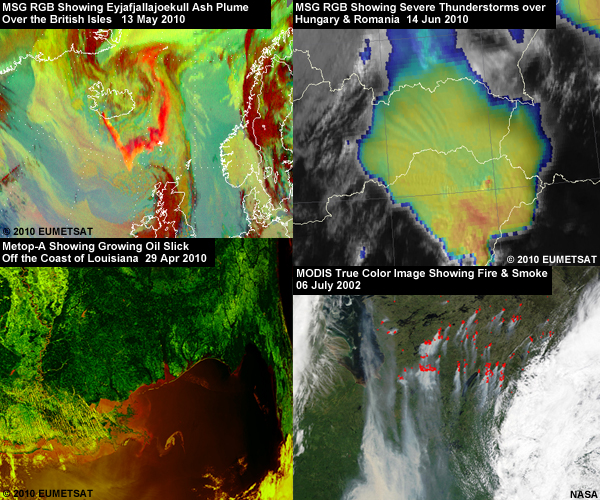
Extreme Weather Events

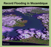
From 2000 to 2009, many extreme weather events occurred around the globe. For example:

• Torrential rains flooded much of Mozambique in 2000, devastating the country for years

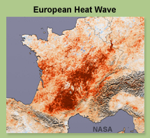
• Europe experienced deadly heat waves in 2003

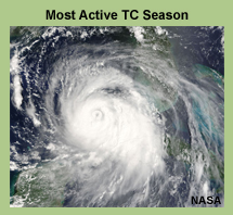
• The most active Atlantic tropical cyclone season on record occurred in 2005

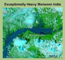
• Exceptionally heavy monsoon rains and floods affected 30 million people in South Asia in 2007

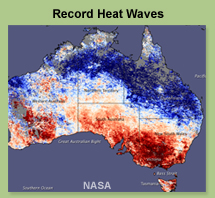
• And Australia experienced record heat waves in 2009

When scientists try to predict these types of extreme weather events, they must try to differentiate between those caused by an unusual confluence of short-term atmospheric (aka weather) phenomena and those related to or exacerbated by climate patterns and cycles. In this module, we'll examine various climate events and their impact on weather. You'll see the important role that Earth-observing satellites play in monitoring them.

Climate and Observing Systems »
A Review of Climate Systems, Part 1

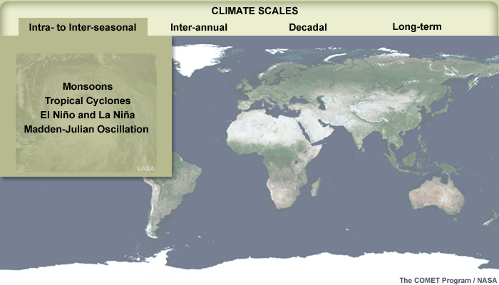
To begin, climate cycles occur on a variety of time and spatial scales.

Intra- to inter-seasonal climate cycles last from weeks to months. Among them are monsoons. These are patterns of atmospheric circulation and rainfall that change seasonally. Monsoons occur each year, with their location and extent determining which areas experience drought or flooding.

The tropical cyclone season is another example. It occurs during the same time frame each year, with variations in the number of storms and their intensity.

El Niño and La Niña are cycles of Pacific Ocean temperature anomalies that affect adjacent climates in distinct and predictable ways. They last from several months to a year.

Finally, the Madden-Julian Oscillation or MJO circles the globe from west to east every 30 to 60 days. It affects rainfall and tropical cyclone development in regions around the world.

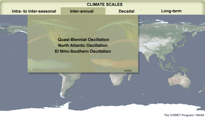
Interannual climate cycles last a year or longer.

Examples include:

• The Quasi-Biennial Oscillation or QBO. This is a reversal of winds in the lower stratosphere. It impacts tropical rainfall patterns, changes the mixing and distribution of ozone and other trace gases in the stratosphere, and interacts with other climate cycles such as ENSO.
• The North Atlantic Oscillation or NAO. This is a fluctuation in pressure patterns, which lasts from months to several years. The NAO influences the westerlies, changes storm and tropical cyclone tracks across the North Atlantic Ocean, and modifies surface temperatures and precipitation for regions around the North Atlantic basin.
• The El Niño-Southern Oscillation (ENSO) climate cycle, which typically lasts from three to five years and includes both an El Niño and a La Niña event. El Niño and La Niña are natural climate patterns that result from interactions between the ocean and the atmosphere and involve abnormal ocean surface temperatures and winds. ENSO impacts regional temperature and rainfall patterns, and contributes to extreme weather events, such as floods and droughts, in many parts of the world.

Decadal climate cycles last ten or more years. Among them is the Pacific Decadal Oscillation. Every twenty to thirty years, the surface waters in the Pacific Ocean north of 20 degrees latitude switch from being relatively cool in the western Pacific and warm in the eastern Pacific to the opposite. This creates a distinct horseshoe pattern of sea surface temperature anomalies. Changes in the PDO can impact droughts and flooding around the Pacific basin and tropical cyclone activity in the Pacific and Atlantic Oceans.

Finally, long-term climate cycles last from hundreds to thousands of years. They span the globe and affect weather and climate at all scales. Examples include ice ages, changes in ocean circulation patterns, and today's observed climate conditions.

Scientists are finding a growing number of connections between climate events at all scales. For example, El Niño and La Niña events affect the distribution of global rainfall and can strengthen or suppress tropical cyclone activity and monsoons. Likewise, the NAO modifies land and ocean temperatures and changes precipitation patterns as it influences storm and tropical cyclone tracks across the North Atlantic.

Recent observed warming of global temperatures may well be exacerbating regional weather extremes and climate trends. For example, warmer temperatures allow for more energy and water vapor in the atmosphere, which can feed into developing storms. The evidence indicates that heavy precipitation events are becoming more frequent in some regions of the world.

Climate and Observing Systems »
A Review of Climate Systems, Part 2

So far, we've looked at weather events and climate cycles that involve interactions between the atmosphere and hydrosphere. But there are actually five overlapping and interacting systems that contribute to climate:

• The atmosphere, which is defined as the layer of air surrounding the Earth that's held in place by gravity. When we discuss weather and climate, we refer to two layers of the atmosphere: the troposphere, which begins at Earth's surface and extends to approximately 9 km at the poles and 17 km at the equator; and the stratosphere, which extends from the top of the troposphere up to about 51 km.

• The biosphere or living system. More specifically, it's the global sum of all ecosystems that supports life on Earth and forms a closed self-regulating system.

• The hydrosphere or water portion of the Earth. It includes snow, ice, and glaciers; and water vapor, clouds, and all forms of precipitation in the atmosphere.

• The cryosphere or ice system. This is the portion of the Earth's surface in which water is in frozen form. It includes sea ice, lake ice, river ice, glaciers, ice caps, ice sheets, and frozen ground.

• And the lithosphere or land system. This is the solid portion of the Earth as compared to the atmosphere and hydrosphere.

Climate and Observing Systems »
Essential Climate Variables

The international science community has organized the Global Climate Observing System or GCOS to measure how the five climate systems are changing and gauge their likely impact on future climate. As part of GCOS, scientists have identified a set of Essential Climate Variables (or ECVs) that should be monitored. As you'll see in the module, environmental satellites play a significant role in this effort.

The Essential Climate Variables are divided into three spheres: atmospheric, terrestrial, and oceanic.

Atmosphere

Surface: Air temperature, wind speed and direction, water vapor, pressure, and the surface radiation budget

Upper-air: Temperature, wind speed and direction, water vapor, cloud properties, and the Earth radiation budget (including solar irradiance, which is energy received from the Sun and its variation by wavelength)

Composition: Carbon dioxide, methane, and other long-lived greenhouse gases, and ozone and aerosols and their precursors

Ocean

Surface: Sea-surface temperature, sea-surface salinity, sea level, sea state, sea ice, surface current, ocean colour, carbon dioxide partial pressure, ocean acidity, and phytoplankton

Sub-surface: Temperature, salinity, current, nutrients, carbon dioxide partial pressure, ocean acidity, oxygen, and tracers

Terrestrial

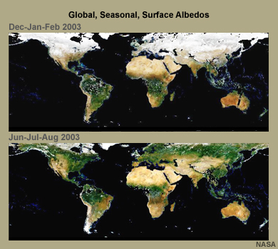
River discharge, water use, groundwater, lakes, snow cover, glaciers and ice caps, ice sheets, permafrost, albedo, land cover (including vegetation type), fraction of absorbed photosynthetically active radiation (FAPAR), leaf area index (LAI), above-ground biomass, soil carbon, fire disturbance, and soil moisture

As scientists have learned more about climate, the list of variables has been updated. For the most current information, visit the GCOS site at http://www.wmo.int/pages/prog/gcos/index.php?name=ObservingSystemsandData.

Climate and Observing Systems »
Observing Systems

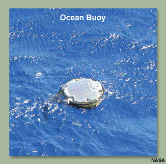
A variety of observing systems monitor the essential climate variables. For example, ocean buoys measure many surface and sub-surface oceanic properties, such as temperature, phytoplankton, nutrients, and currents.

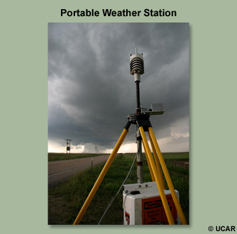
Ground-based weather stations measure atmospheric properties, such as surface temperature and moisture, pressure, precipitation, and wind speed and direction.

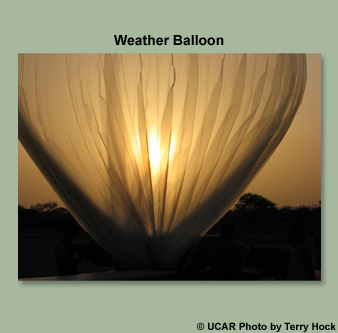
Weather balloons measure temperature, water vapor, and wind as they rise through the troposphere and stratosphere.

Instrumented boreholes at high latitudes and in high mountainous regions monitor the depth and thermal structure of permafrost and seasonally frozen ground.

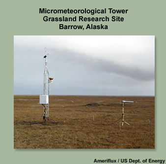
And micrometeorological towers take continuous CO2 flux measurements to estimate the carbon budget for a variety of ecosystems.

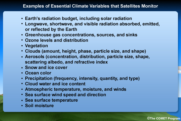
Satellites are in the unique position of being able to provide a broad, spatially consistent, and continuous global sampling of many essential climate variables. Some of these variables complement those from other observing systems, while others are unique. Not surprisingly, some of the best results are produced when many types of observations are combined. Examples include measurements of atmospheric moisture and temperature, precipitation, sea surface height, and ocean phytoplankton.

Here are some of the ECVs that satellites monitor.

Scientists use satellite observations to understand, detect, monitor, and predict various weather and climate events. For example:

• Observations of sea surface temperature and atmospheric winds are used to help predict the number and intensity of storms within a tropical cyclone season
• Ozone measurements help monitor the behavior of the Quasi-Biennial Oscillation and even predict El Niño and La Niña events
• Observations of cold convective cloud tops and upper atmospheric wind anomalies help weather forecasters confirm where the Madden-Julian Oscillation is supporting active tropical convection; determine if it is aiding or suppressing tropical cyclone activity; and determine if it is affecting the onset of the Indian monsoon

Satellites ultimately help us answer complex questions about climate change and its impact on society. For example, they help us determine:

• The state of the global climate system and how it varies
• The causes of climate change and the extent to which natural and human-related forcings contribute
• How climate will change in the future and how well we will be able to predict it
• If weather events will become more frequent or extreme
• Where the impacts of extreme weather events and climate change will be felt around the world

Climate and Observing Systems »
About the Module

Whether you are a forecaster who uses satellite products on a daily basis and is curious about their contribution to climate monitoring, a student studying meteorology or climate, or a decision or policy maker who needs background information to make informed choices, this module will help you to understand:

• The various scales of climate, examples of climate events, and their impacts
• The weather and climate variables that satellites observe and the climate cycles that this enables them to monitor
• The benefits and challenges of monitoring climate with satellites

The module is structured as follows:

• Section 2 (How Satellites Measure ECVs) describes meteorological and environmental satellites and how they observe key atmospheric features that are common to most climate cycles; this information is basic but critical for understanding the rest of the module
• Sections 3 through 5 (Intra- to Inter-Seasonal, Inter-Annual, and Decadal to Long-Term Climate) are arranged by climate scale; they explore events at each scale and the contributions that satellites make to their monitoring and prediction
• Section 6 (Challenges for Satellite Monitoring) describes the challenges of monitoring climate with satellites

How Satellites Measure ECVs »
Overview, Part 1

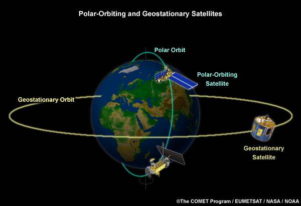
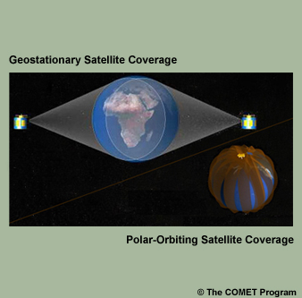
Two distinct but complementary weather and environmental satellite systems work together to provide Earth science data to weather forecasters, climate researchers, and global decision makers. The systems include geostationary (or GEO) and low earth orbiting (or LEO) satellites. Polar-orbiting satellites are a subset of the latter.

Polar-orbiting satellites fly in relatively low orbits, several hundred kilometers above Earth's surface. This allows for high-resolution imaging across all latitudes, which is important for observing atmospheric, land, and ocean features.

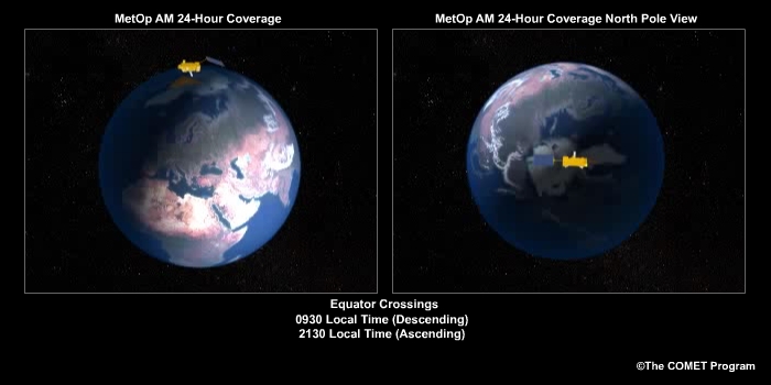
Polar orbiters observe most locations twice daily, except at higher latitudes where their orbits overlap and coverage is more frequent. The polar orbiters used for monitoring weather and the environment fly in sun-synchronous orbits. (Their orbits are fixed with respect to the Sun, with the Earth rotating below them.) This allows each satellite to view a fixed location every 12 hours at a specific time of day or night. While this limits the ability of polar orbiters to monitor day-night variations and rapidly changing weather at a useful interval, it make them well suited for monitoring long-term changes that are not dependent on the time of day.

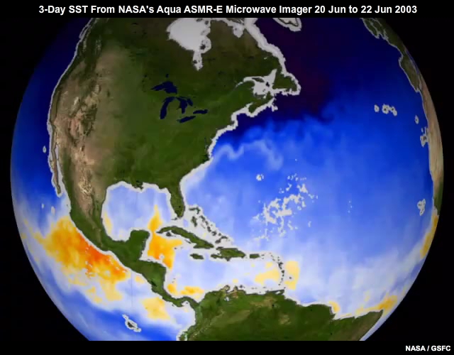
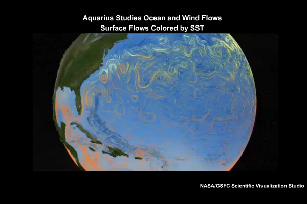
This animation of sea surface temperatures (SSTs) illustrates the daily coverage and detail provided by the AMSR-E microwave instrument on NASA's Aqua polar orbiter. The yellow- and orange-shaded waters are warm enough to support the generation of tropical cyclones. Daily images like this help scientists monitor the slow evolution of ocean eddies, currents, and abnormally warm or cool regions that may be linked to climate cycles such as ENSO.

How Satellites Measure ECVs »
Overview, Part 2

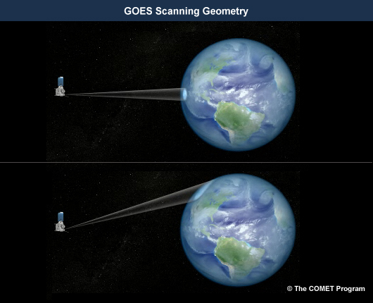
Geostationary satellites fly in higher orbits than their polar-orbiting counterparts, at approximately 35,000 km above the Earth's surface. At this height, they match the Earth's rotation, which allows them to hover over a fixed location above the equator. This also lets them view specific regions of the Earth at 30-minute intervals or better. However, their fixed position above the equator limits their view of the polar regions beyond 70 degrees latitude.

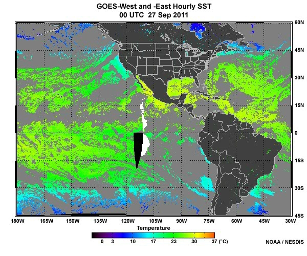
With their frequent updates and relatively high-resolution infrared sensors, geostationary satellites can provide a more complete view of, for example, evolving sea surface temperature patterns. This lets climate scientists better monitor day-night changes in weather patterns that are influenced by SST and ocean currents, such as convection and tropical cyclones.

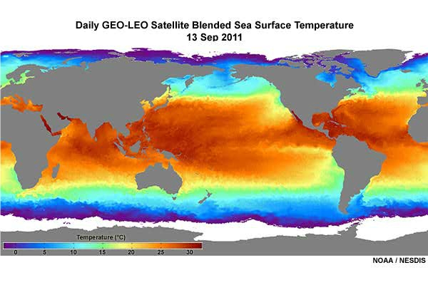
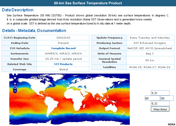
By leveraging the capabilities of both GEO and LEO satellites, scientists can better understand the connections between weather and climate. Blended satellite products, such as this SST product, take advantage of the strengths of both types of satellite, providing high-resolution global coverage and more frequent updates.

How Satellites Measure ECVs »
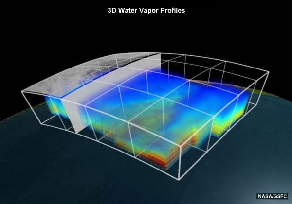
Monitoring Atmospheric Elements

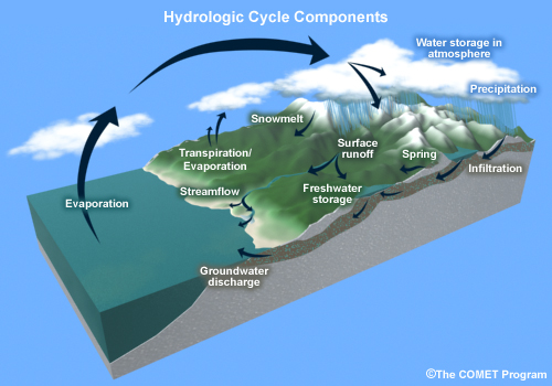
Atmospheric water vapor, clouds, and precipitation are important components of the hydrologic cycle and climate at all scales: from seasonal patterns of rainfall and tropical cyclone activity; to storm patterns affected by inter-annual and decadal cycles; to long-term climate trends and the Earth's energy budget.

• True Color Composite
• Infrared Cloud Phase
• Cloud Effective Radius
• Cloud Optical Thickness

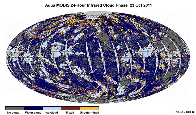
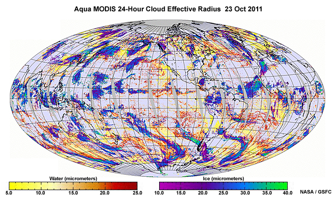
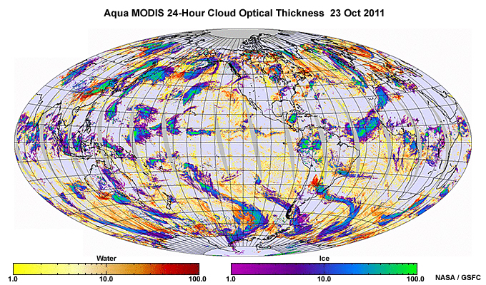
Satellite measurements of cloud coverage and cloud properties help scientists better understand how the different climate oscillations impact cloud development and distribution. And global cloud cover is a key factor in understanding future climate conditions.

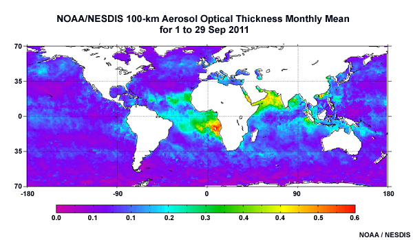
Aerosols are important to the climate system because of their potential to influence cloud development and their role in the Earth's energy budget. Aerosols are an important consideration for climate on many scales, from seasonal forecasts of tropical cyclones, rainfall, and temperature, to longer-term climate variability and change. As we will see, satellites play an important role in monitoring and helping us understand how aerosols are distributed in the atmosphere, their sources and sinks, and their impact on cloud development and precipitation.

The remainder of this section looks at how satellites observe these atmospheric elements.

How Satellites Measure ECVs »
Atmospheric Water Vapor, Clouds, and Precipitation

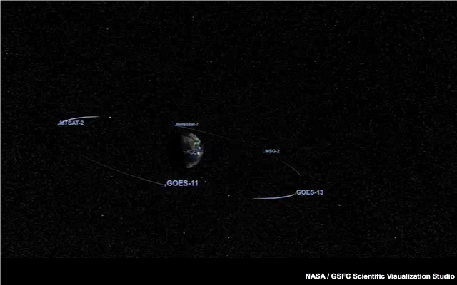
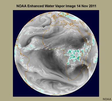
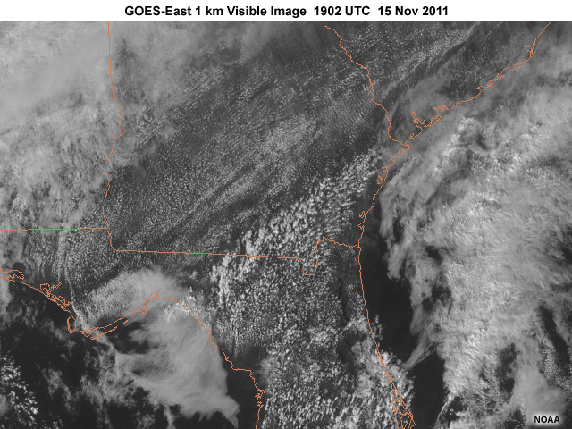
Constellations of geostationary and polar-orbiting satellites collectively measure atmospheric water vapor, clouds, and precipitation.

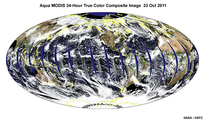
Observations from several geostationary satellites are routinely stitched together, enabling scientists to track the movement of atmospheric moisture, assess day-night changes in Earth's cloud cover, and monitor heavy rainfall events as they unfold.

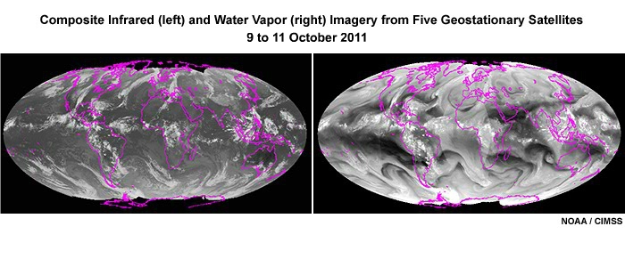
These animations, assembled from five geostationary satellites, emphasize Earth's clouds and water vapor as they evolve over a three-day period.

With lower orbits and multisensor capabilities, polar orbiters provide more detailed information about cloud and aerosol properties, precipitation rates, and important atmospheric gases, such as water vapor, carbon dioxide, ozone, and methane. While their orbits limit the number of times that each location is observed, they provide crucial views of the polar regions that lie beyond the reach of geostationary satellites.

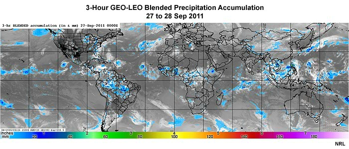
When observations from geostationary and polar-orbiting satellites are combined, as in this blended rainfall accumulation product, the strengths of each observing system are realized in a single product.

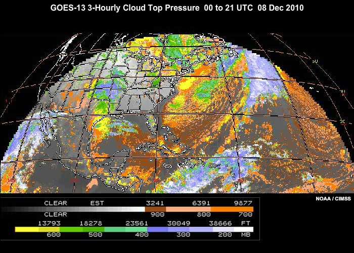
The International Satellite Cloud Climatology Project (ISCCP) collects observations from all available meteorological satellites. It analyzes the global distribution of clouds, their properties, and their diurnal, seasonal, and inter-annual variations. These observations are processed into products used to study the role of clouds in climate as well as the global water cycle.

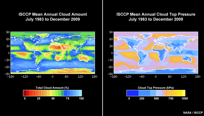
These analyses show mean annual cloud cover and cloud top pressure from 1983 to 2008. Notice how cloudy Earth's oceans are relative to the large land masses. This highlights the important role that satellites play in observing our relatively data-sparse ocean regions.

For more information on atmospheric water vapor, clouds, and precipitation, see the COMET module Microwave Remote Sensing: Clouds, Precipitation, and Water Vapor.

How Satellites Measure ECVs »
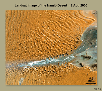
Aerosols and Dust

Atmospheric concentrations of aerosols and dust from sources such as transportation, industry, agriculture, land use, and dust storms not only pose serious concerns for human health but also affect weather and climate.

Aerosols and dust can have a significant influence on precipitating clouds and tropical disturbances. Scientists are keenly interested in what causes tropical disturbances to blossom into tropical cyclones or dissipate. They believe that dust storms from the Sahara may stifle storm development by injecting a layer of dust and dry air, known as the Saharan Air Layer or SAL, into the low- to mid-level easterly jet stream. They hypothesize that dry air and increased vertical wind shear weaken the intensity of convection while dust inhibits its development by reducing solar heating of the ocean surface.

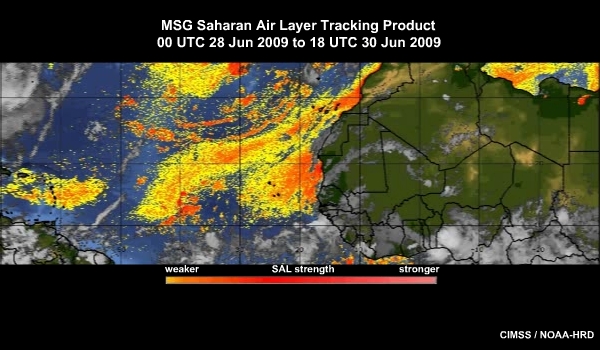
But Saharan dust may also seed the clouds, which could then invigorate convection and promote storm formation. Satellites that map dust and other aerosols in close proximity to developing storms are helping scientists decide whether dust stifles or strengthens storms.

The SAL product is very useful in that it clearly shows the movement and extent of dry air. This animation, produced from Meteosat-9 observations, shows pulses of dust in orange and darker reds as they moved westward off the West African coast on 30 June 2009.

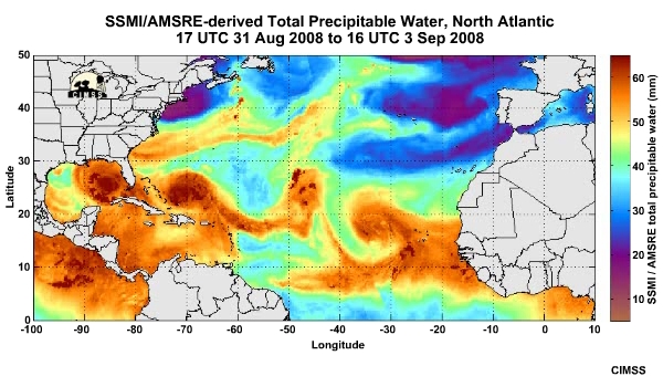
The dry air intrusions associated with the Saharan Air Layer can also be monitored with satellite instruments that measure the atmosphere's total moisture content. For example, this Total Precipitable Water product, made by merging data from GEO and LEO satellites, highlights dry air as it moved westward around the northern perimeter of tropical storm Hanna on 2 to 3 September 2008.

For more information on atmospheric dust, see the COMET module Forecasting Dust Storms, Version 2.

Intra- to Inter-Seasonal Climate »
About the Section

This section explores some of the phenomena that satellites can monitor on intra-seasonal and seasonal climate scales, that is, from weeks to months. We will identify the key weather and climate variables that constitute these phenomena and see how satellites observe them.

Intra- to Inter-Seasonal Climate »
El Niño and La Niña

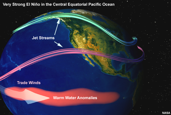
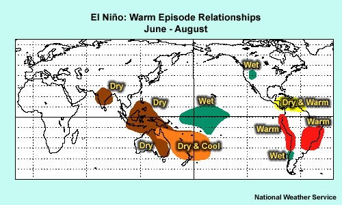
El Niño and La Niña are natural climate patterns that result from interactions between the ocean and the atmosphere. Both involve anomalies in ocean surface temperatures and winds, resulting in weather extremes around the world.

During El Niño events, unusually warm equatorial water off the west coast of South America is accompanied by weaker than average easterly trade winds.

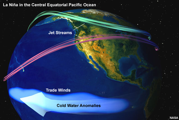
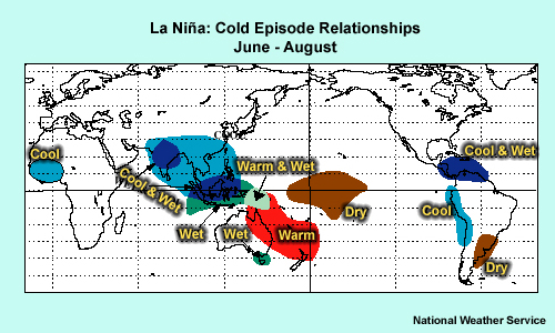
During the opposite phase, La Niña, equatorial water becomes unusually cold and the easterly trade winds blow stronger.

Together with a neutral phase, these patterns oscillate in a phenomenon called the El Niño-Southern Oscillation cycle. A typical El Niño or La Niña lasts several months to a year, while the full ENSO can take three to five years to run its course.

El Niño and La Niña affect regional climate patterns in distinct and reasonably predictable ways. For example, the southern United States tends to be wetter and cooler than average in El Niño years, while northeastern South America is drier. Many groups need improved predictions of the weather influenced by these climate fluctuations so they can plan for their impacts. These impacts can include increases in the severity of regional drought and flooding patterns, diminished or enhanced agricultural productivity, changes in regional fish populations, threats to human life, and significant property damage.

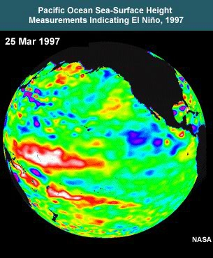
Satellites have much to offer when it comes to improving our monitoring and prediction capabilities. By monitoring sea surface temperature and precipitation patterns, satellites help us detect and forecast the onset, strength, and duration of El Niño and La Niña events. In fact, satellites are the only system capable of observing global sea surface temperatures (SSTs) with the coverage and accuracy needed to monitor and predict ENSO events.

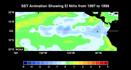
This SST anomaly product created from satellite data shows the Pacific Ocean during the strong 1997 to 1998 El Niño event. Notice the spread of above-average SSTs from the west coast of South America westward along the equator as a strong El Niño established itself during the summer of 1997. By late winter and the early spring of 1998, the ribbon of warmer waters began to cool, signaling the weakening of the El Niño. Products like this help climate and weather forecasters anticipate how El Niño and La Niña will unfold and how long they may last.

For more information on El Niño and the ENSO cycle, see the COMET modules The El Niño-Southern Oscillation (ENSO) Cycle, and ENSO and Beyond. For more information on monitoring the ocean from satellites, see COMET 's Jason-2: Using Satellite Altimetry to Monitor the Ocean module.

Intra- to Inter-Seasonal Climate »
South Asian Monsoon

In the Northern Hemisphere summer, hot air rising from the Indian sub-continent pulls in moist air from the Indian Ocean, deluging the Indian sub-continent with its annual monsoon. The location and extent of the rainfall determines which areas experience drought or flooding.

Satellites help predict which scenario is more likely. The distribution of global rainfall is affected by the ENSO phenomenon, with the monsoon generally producing less rainfall in El Niño years and more rainfall in La Niña years.

Since satellites can detect signs of an El Niño or La Niña event and confirm when one is underway, they help predict whether an excess or shortfall of rain is likely and where.

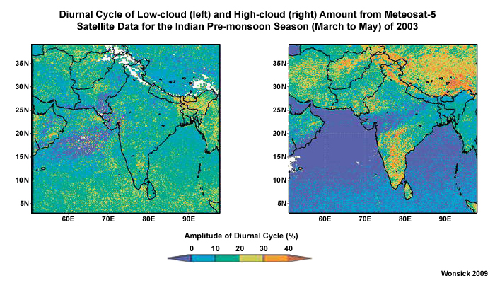
Satellites also help monitor the onset of monsoons by observing spatial and temporal changes in daily cloud patterns and cloud types across the region. Geostationary satellites are particularly useful for monitoring cloud coverage given the pronounced change in day-night coverage. For example, there's little variation during the pre-monsoon season.

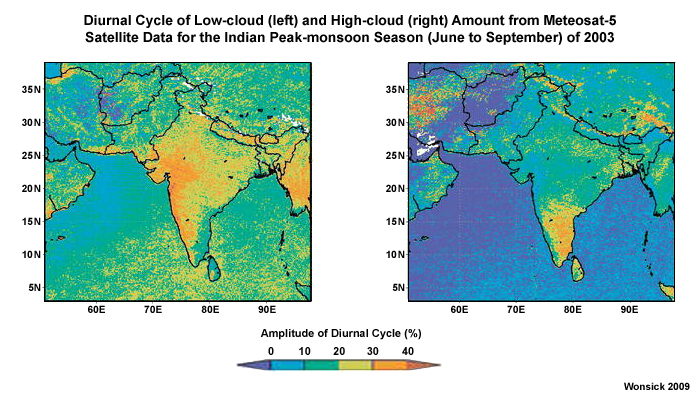
But day/night cloud cover increases significantly across the Indian sub-continent during the peak monsoon season.

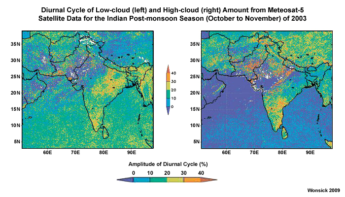
It then drops off during the post-monsoon season (although there's a noticeable peak in afternoon cloud cover over land).

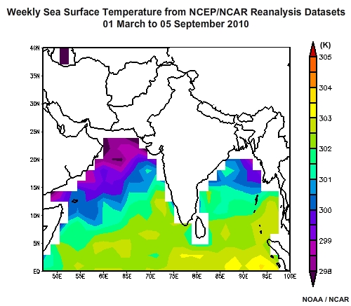
Satellite observations of SSTs and lower tropospheric temperatures over the Arabian Sea and Indian Ocean off the East African coast help forecasters improve predictions of the monsoon season.

For example, when the lower oceanic troposphere becomes noticeably warmer and more unstable, conditions are ripe for an upward release of moisture. This, in turn, supports the development of clouds and precipitation, and signals the onset of the active phase of the summer monsoon.

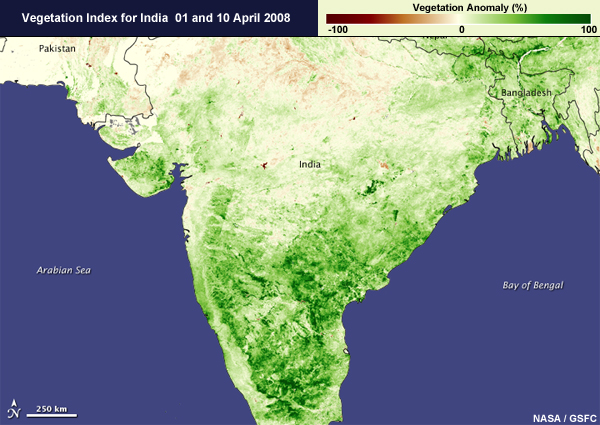
Satellites also provide information about surface conditions during and after monsoon events. For example, this satellite product shows dense vegetation conditions after the monsoon of 2008, which followed a La Niña event. Green indicates above-average vegetation, brown below-average.

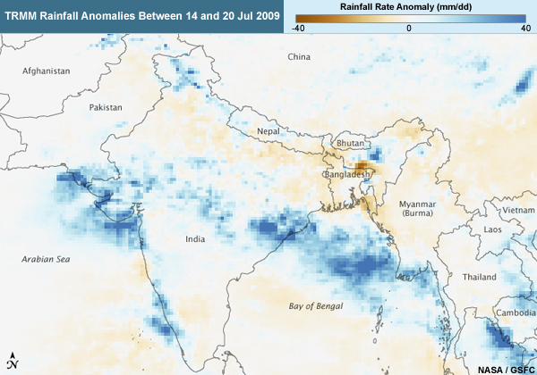
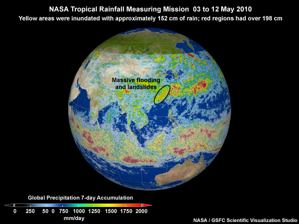
NASA's Tropical Rainfall Measuring Mission or TRMM satellite provided the observations for this image of rainfall anomalies during the 2009 monsoon rains. That was an El Niño year, with little rainfall over many parts of India except a broad band over center of the country.

Observations from the TRMM and upcoming Global Precipitation Measurement mission satellites are turned into precipitation products for use in short-term forecasts and the monitoring of longer-term trends.

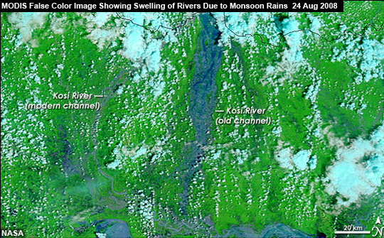
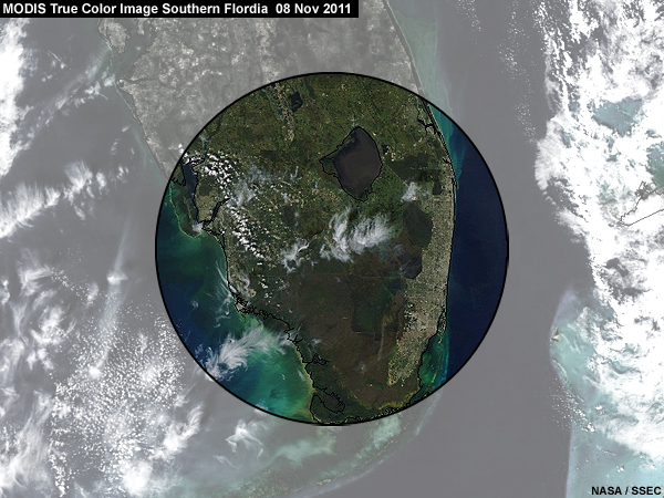
Finally, MODIS false color images from NASA's Terra and Aqua satellites provide evidence of the extent to which flooding has occurred. This image shows how India's Kosi River burst its banks in August 2008 and flowed into a channel that had been abandoned more than 200 years earlier. More than a million people fled their homes in a region unaccustomed to flooding.

Intra- to Inter-Seasonal Climate »
Madden-Julian Oscillation

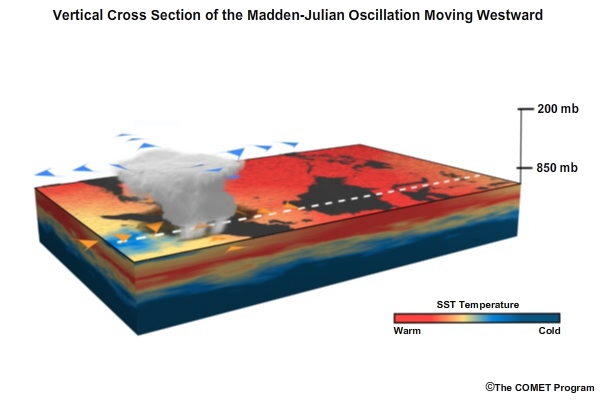
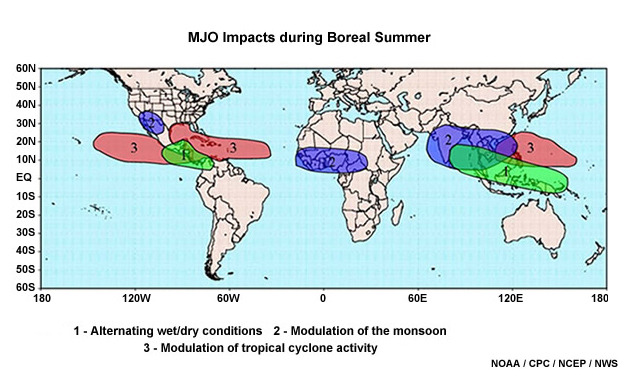
The Madden-Julian Oscillation or MJO is the largest source of intra-seasonal variability in the tropics. The MJO is an oscillating pattern of winds, humidity, sea-surface temperature, and ascending or descending air that enhances, stifles, or suppresses convection and precipitation.

The MJO phenomenon marches slowly from west to east (at approximately 5 meters per second) over 30- to 60-day periods. It is most prominent in the Indian and Pacific Oceans but is also found in the tropical Atlantic Ocean.

• Summer
• Winter

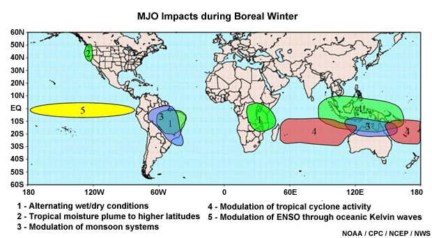
The MJO varies considerably between years, with the oscillation strong in some years and weaker in others. Scientists believe that these cyclical variations may be linked to the ENSO phenomenon. But there's also mounting evidence that the MJO influences the ENSO cycle too. The surface winds associated with the MJO can play a role in the development, intensification, and termination of El Niño and La Niña events.

The active or wet phase of the MJO that supports convection and precipitation encourages the development of tropical cyclones, while the dry phase has a suppressing effect. Because the MJO is normally in opposite phases in the Pacific and Atlantic Basins at any given time, there's an inverse relationship between tropical cyclone activity in the western north Pacific and the north Atlantic Oceans. When one region is active, the other tends to be quieter and vice versa.

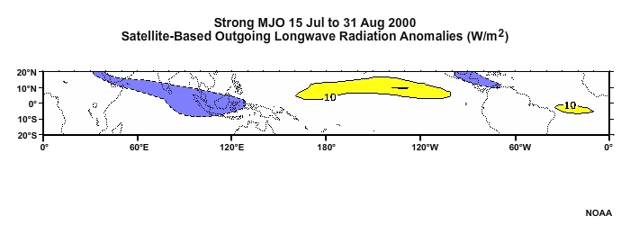
Satellite-based infrared observations help forecasters track enhanced thunderstorm activity as it moves eastward with the active phase of the MJO. The stronger the active region of thunderstorms, the colder the cloud tops and the lower the amount of outgoing longwave radiation (OLR). This satellite-based animation shows a series of diminished and enhanced OLR blobs as they move eastward along the equator from the Indian Ocean into the Pacific. The blue areas (cold cloud tops) indicate where thunderstorm activity is enhanced. The red areas show where it's diminished.

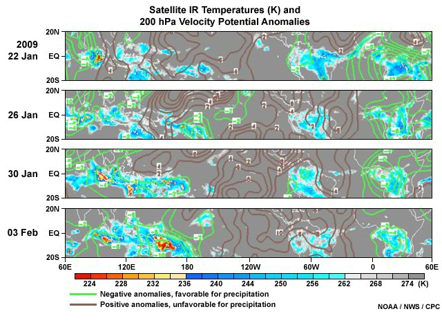
Even when the MJO is less convectively active, such as over the Atlantic Ocean, it can still be tracked using satellite-derived 200-hPa velocity potential or water vapor imagery. In this plot of infrared satellite observations and 200-hPa velocity potential anomalies, the green contours correspond to regions where convection is enhanced. The brown contours show regions where convection is suppressed.

Beyond the tropics, the MJO can impact North American weather patterns over a one- to two-month period as shown here in a winter example. The graphic shows a typical setup for a heavy wintertime precipitation event over the West Coast of the U.S. Enhanced tropical convection supported by the MJO results in a deep plume of moisture that's transported north and east towards North America. It can support several days of heavy rains and possible flooding.

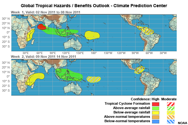
The MJO's global nature, short duration, and slow eastward movement make it a valuable source of predictability for regional weather and climate. By applying statistical techniques to satellite data, forecasters can identify the MJO and extrapolate its eastward movement. These satellite-based tools are important inputs for NOAA's Global Tropical Hazards Assessment, which provides weekly updates and forecasts of MJO-related impacts including tropical cyclone activity and abnormal rainfall patterns.

For more on the MJO, see the COMET module by Madden himself, The Madden Julian Oscillation Lifecycle.

Inter-Annual Climate »
Introduction

Climate oscillations on inter-annual to decadal time scales can modify regional and global weather patterns over periods lasting weeks to many months. Some of the more prominent oscillations include the North Atlantic Oscillation and the Quasi-Biennial Oscillation, which we will discuss in this section. We will also explore the climate variables related to these oscillations, such as sea surface temperature, sea surface height, atmospheric pressure, and ozone. And of course, we will look at the role that satellites play in monitoring the variables and helping scientists predict the oscillations and their impacts.

Inter-Annual Climate »
Quasi-Biennial Oscillation

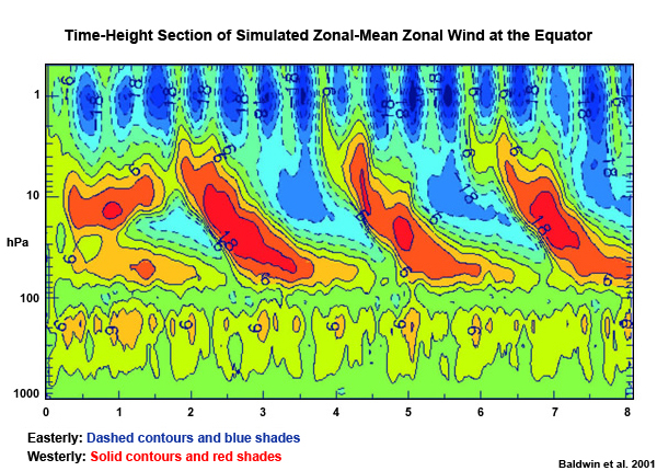
The Quasi-Biennial Oscillation or QBO is a regular reversal of the winds in the lower stratosphere over the tropics. As the graphic shows, the winds switch between blowing from the east to blowing from the west roughly every 15 months or so. At their strongest, the easterly winds (shown in blue) blow about twice as hard as the westerly winds (shown in red).

Scientists are investigating connections between the QBO and other climate cycles. The QBO clearly impacts tropical rainfall patterns and ENSO but so far, no definitive connection has been found with tropical cyclone activity.

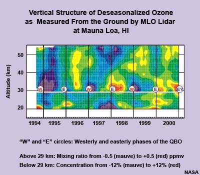
QBO cycles also impact the mixing and distribution of ozone and other trace gases in the atmosphere. This first plot shows the vertical structure of ozone as measured from the ground at the Mauna Loa observatory in Hawaii.

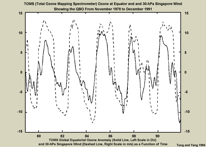
The second plot shows total column ozone measured from the TOMS (Total Ozone Mapping Spectrometer) instrument, which flew on the NIMBUS-7 satellite from 1978 to 1993. Notice the correlation between the alternating west-east stratospheric winds and ozone during each QBO cycle.

It's clear from these observations that monitoring changes in atmospheric ozone in the tropics helps scientists study the QBO's behavior and understand how it affects the movement of other trace gases, such as sulfur dioxide and nitrogen oxides.

If you are interested in the following topics, click the links below. If you want to skip this information, just proceed to the next page.

• More about Ozone Monitoring
• How Satellites Measure Winds and Other Variables

Satellites have been monitoring ozone levels since the late 1970s, starting with the TOMS instrument on NIMBUS-7. Vertical profiling of ozone was made feasible in the 1990s with ERS-1 and -2 and the GOME instruments that flew on follow-on satellite missions. Further improvements followed in the next decade with instruments such as SCIAMACHY, OMI, AIRS, IASI, and GOME-2. The U.S. NPP and future polar-orbiting satellites will boost our ability to monitor the QBO even more. Their ozone profilers will be able to routinely measure the vertical structure of ozone in the stratosphere with improved accuracy and vertical resolution. This is especially important in the lower stratosphere (30 to 40 km) where a rich ozone layer absorbs 97 to 99 percent of the Sun's damaging ultraviolet light.

Research has also shown that the unique temperature and wind structure associated with the QBO can be detected by satellite radiance and wind measurements. By combining and analyzing these different satellite measurements, scientists are validating and improving numerical predictions of the QBO and its effects on tropical weather patterns.

How do satellites obtain the vertical profiles of winds, temperature, moisture, and trace gases such as ozone that are critical to understanding and predicting the QBO and other climate cycles?

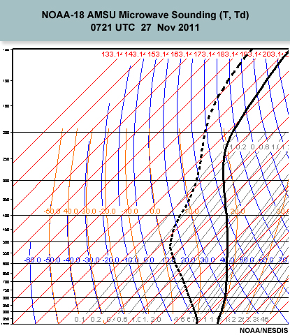
Constellations of polar-orbiting satellites, such as EUMETSAT's Metop, NOAA's POES, and China's Fengyun series, carry infrared and microwave sounders designed to profile atmospheric temperature and moisture in the troposphere and stratosphere.

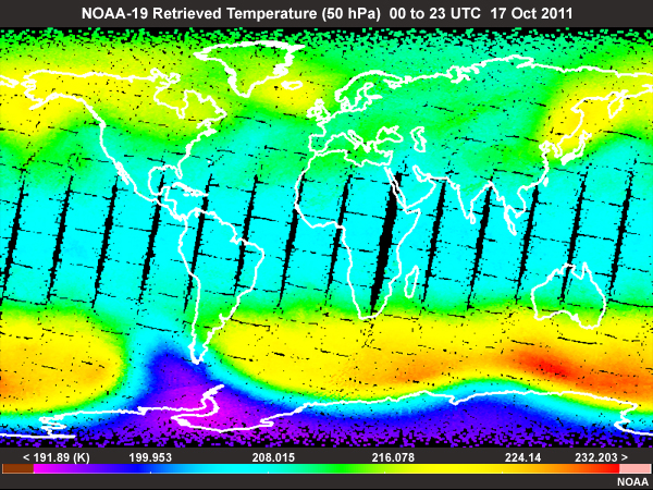
This plot of 50-hPa temperatures obtained from the NOAA-19 satellite highlights the global coverage obtained from just one polar orbiter every twelve hours. The black diagonal stripes are gaps between orbits. The temperature patterns seen in this plot are indicative of the region of the stratosphere where the QBO dominates (between 10 and 70 hPa).

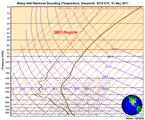
Here we see one of the thousands of profiles generated from one satellite in a twelve-hour period. The region of the stratosphere where the QBO dominates (between 10 and 70 hPa) is highlighted.

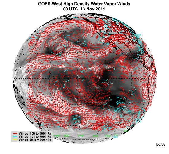
Satellites also measure atmospheric winds by watching the movement of clouds and water vapor.

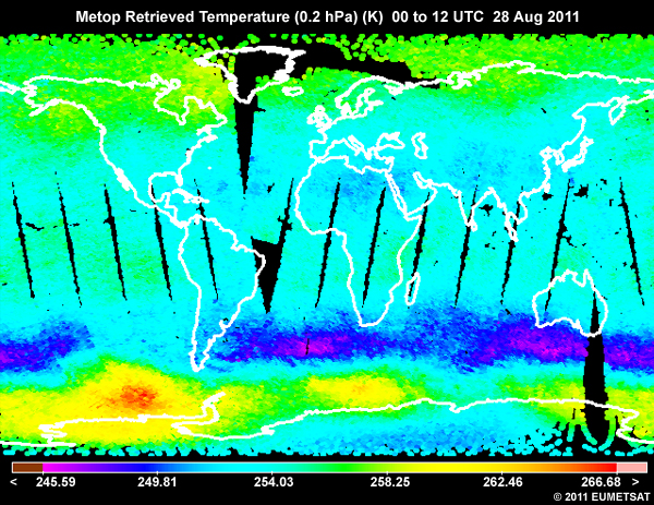
Satellite observations of atmospheric temperature gradients are used to make indirect observations of winds in the troposphere and stratosphere. This Metop temperature product is for 0.2 hPa (~35 km), the level in the lower stratosphere where some of the stronger QBO-related temperature anomalies are typically found.

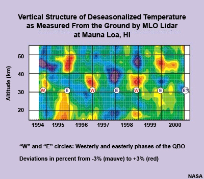
When analyses such as this are transformed into a time series, such as the temperature anomaly cross section at Mauna Loa, Hawaii, we see the strong linkage between temperature and QBO wind reversals, especially between 30 to 40 km.

Inter-Annual Climate »
North Atlantic Oscillation

• Negative NAO
• Positive NAO

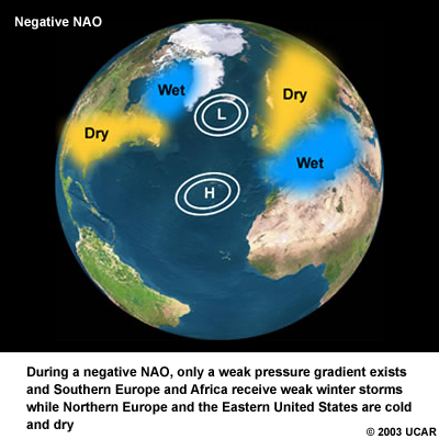
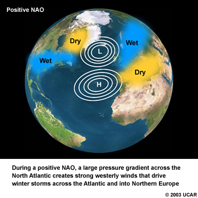
The North Atlantic Oscillation or NAO is a cycle that repeats on the order of months to several years. The NAO is a fluctuation in the intensity of the Iceland low-pressure zone southeast of Greenland and the subtropical high-pressure zone northwest of Africa, over the Azores.

The fluctuations and movements in this pressure pattern control the strength and direction of the westerlies and storm tracks across the North Atlantic. This impacts temperature and precipitation from New England to Western Europe, across Siberia, and from the eastern Mediterranean southward to West Africa.

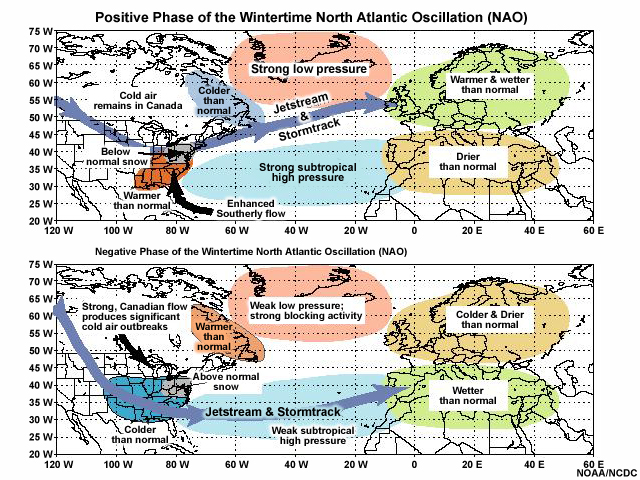
Researchers hypothesize that the phase of the NAO affects the movement of Atlantic hurricanes. When the Azores high is farther south, storms are steered into the Caribbean and Gulf of Mexico, whereas a more northern position allows them to track up the North American Atlantic Coast.

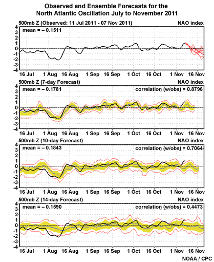
The NAO has been monitored from land and sea since the 1800s. Our monitoring capabilities have dramatically improved in recent years through the use of satellites. They enable us to observe the NAO more continuously in time and space and improve our understanding of its behavior.

Satellites monitor the NAO by:

• Observing changes in sea level caused by fluctuations of the NAO and the variations in sea surface temperature that go with it. This is helping scientists begin to understand the role that the ocean plays in the NAO.
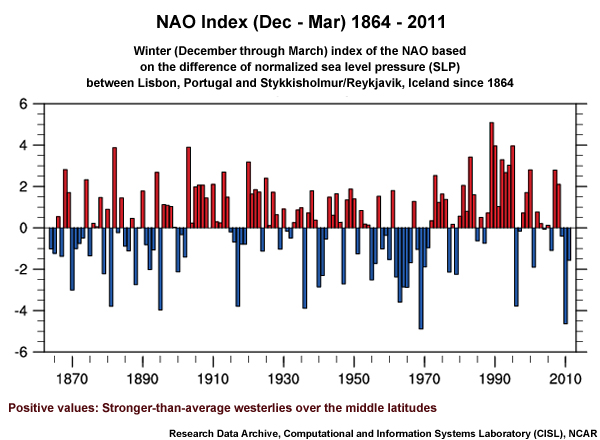
• Detecting fluctuations in large-scale atmospheric pressure patterns across the Atlantic basin. By analyzing these fluctuations, scientists have created the NAO index which is used to monitor and make short-range predictions of the NAO.

Decadal to Long-Term Climate »
About this Section

Longer-term climate variations and changes span the globe and can last from decades to hundreds and even thousands of years, affecting weather and climate at all scales. Examples include:

• Multi-decadal cycles of tropical cyclone activity and ocean-atmosphere fluctuations such as the Pacific Decadal Oscillation or PDO
• Long-term changes in global precipitation patterns that lead to regional flooding and drought
• Increases in greenhouse gases that accelerate sea level rise and the melting of glaciers and polar ice caps
• Changes in ocean circulation and heat storage that affect regional and global climate
• Changes in stratospheric ozone, which shields life from harmful ultraviolet radiation

The dynamics and interactions that influence long-term climate variability involve variables from all of Earth's spheres (the atmosphere, biosphere, hydrosphere, cryosphere, and lithosphere). Given the global nature of long-term climate variability, satellites play a crucial role in monitoring many of the variables. They also help build a seamless data record that provides a "best estimate" of the climate's mean state, its variability, its extremes, and possible long-term trends at any given time and place.

In this section, we will look at the PDO and then examine key variables that are related to long-term climate, such as solar radiation and atmospheric temperature. We'll see how satellites help with:

• Defining and extending the climate record
• Improving our understanding of climate variability and long-term changes in the climate’s mean state, and
• Understanding the balance between Earth’s natural variability and changes attributed to human activity

Decadal to Long-Term Climate »
Pacific Decadal Oscillation

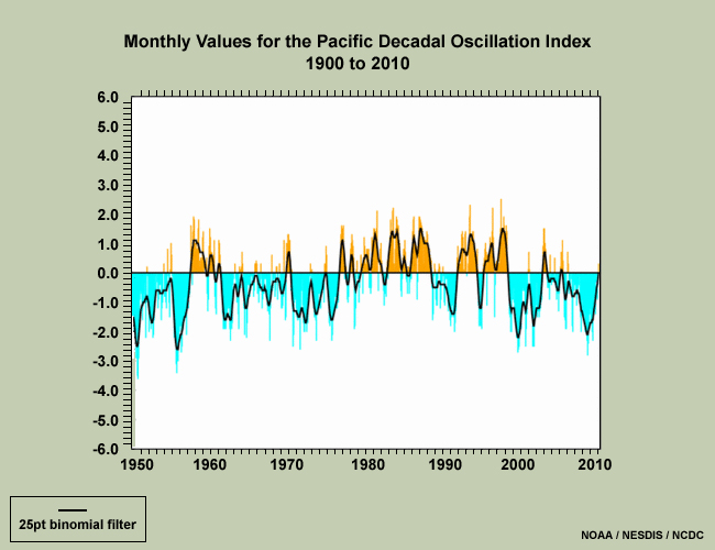
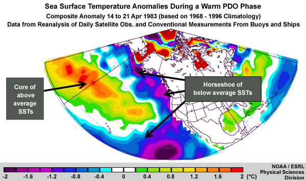
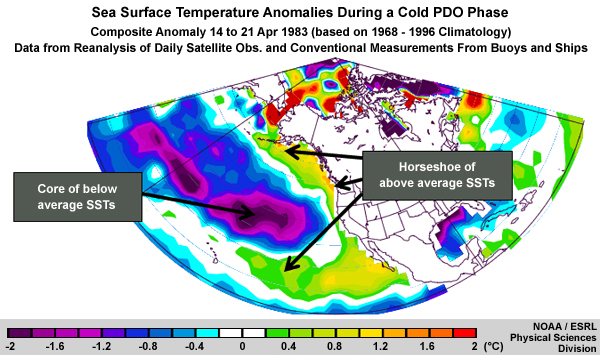
The Pacific Decadal Oscillation or PDO is a pattern of relatively warm or cool surface waters in the Pacific Ocean north of 20 degrees latitude. Every twenty to thirty years, the water switches from being cooler than average in the western Pacific and warmer than average in the eastern Pacific (the "warm phase") to the opposite (the "cool phase").

• Warm Phase
• Cold Phase

This creates a distinct horseshoe pattern of sea surface temperature anomalies. Data show that most of the anomalies are relatively small, ranging from a few tenths to several tenths of a degree Celsius. This illustrates the importance of accurate SST observations for capturing an anomaly or change in anomalies over time. As these plots show, satellites are well suited for this task. They were constructed from a reanalysis of daily satellite observations and measurements from buoys and ships.

Shifts in the position of colder and warmer ocean water alter upper-level atmospheric winds and the path of the jet stream. Changes in the jet stream, in turn, alter global weather patterns and impact regional climate.

Scientists hypothesize that the PDO can intensify or diminish the impacts of an El Niño or La Niña depending on their relative phases.

For example, when the PDO is in its warm phase, western portions of North America tend to experience wetter winters during El Niño events and closer to average precipitation during La Niña winters. This combination of climatic conditions may improve water supplies since winter precipitation is typically responsible for most water replenishment in the Western U.S.

When the PDO is in its cool phase, western portions of North America may experience drier La Niña winters. And El Niño winters may have closer to average precipitation, not the excessive precipitation that's more typical. This reduces the long-term average precipitation and increases the chances of below-normal precipitation in winter.

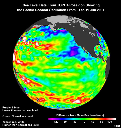
Altimetry satellites, such as the Jason series, measure sea surface height. In this 10-day altimetry composite, the yellows and reds in the Western Pacific are higher-than-normal sea levels (warmer waters). The blues and magentas in the Eastern Pacific are lower-than-normal sea levels (cooler waters). (As you'll recall, warmer water expands and cooler water contracts.)

Notice the strong similarity between the sea surface height patterns and the SST patterns that we looked at earlier. When scientists combine both types of data, they are better able to understand what happens to the ocean surface when temperatures shift away from average conditions during an active PDO.

Although ocean temperature and sea height are closely correlated, there are often subtle differences that point to other interactions that may be taking place. Satellite observations are crucial for discerning these differences. They're also essential for understanding how the PDO interacts with ocean dynamics such as currents and eddies, and other oceanic and atmospheric oscillations, such as ENSO.

Decadal to Long-Term Climate »
Solar Radiation and Earth's Radiation Budget

The Sun's output is usually quite steady in the short term, around a decade. But it can change over many years and affect Earth's climate. Earth's atmosphere obscures our view of this phenomenon, making satellites in orbit above our atmosphere critical for observing the changes.

Satellites are ideally positioned to observe changes in radiation flux or energy in the Earth-atmosphere system. Some of the Sun's energy is reflected by clouds, aerosols, and the Earth itself. The rest is absorbed and re-emitted by land, water, clouds, and the atmosphere. The planet as a whole warms when the global net radiation balance is positive and cools when it's negative. Satellites can measure the radiation budget particularly well at the top of Earth's atmosphere and monitor it over time, which is critical for detecting long-term climate tendencies. The current challenge is to be able to quantify how each of the atmospheric, land, and ocean systems are responding to net increases and decreases in the Earth's overall radiation budget. This requires more information and improved observing systems.

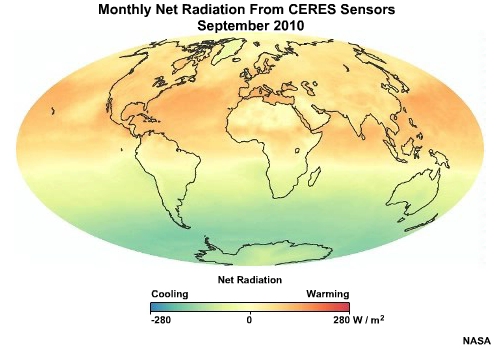
This animation from the CERES instrument on NASA's Terra and Aqua satellites shows how satellites can measure net radiation (the balance between incoming solar and outgoing Earth-atmosphere energy at the top of the atmosphere). A net positive should lead to warming, a net negative to cooling. In the animation, areas that receive more energy than they send back to space are red, while those that receive less energy are green. As expected, the pattern changes seasonally, with the summer hemisphere receiving more sunlight than the winter hemisphere.

Another set of satellite instruments measure the Sun's total energy output, the partitioning of its energy by wavelength, and the way in which the Sun's input to the Earth's climate system changes over time. The first of these instruments flew on the ERBE (Earth Radiation Budget Experiment) satellites of the 1980s and NASA's Solar Radiation and Climate Experiment (SORCE) mission launched in 2003. They are being carried forward by the U.S. NPP and future polar-orbiting satellites, and EUMETSAT's geostationary MSG satellites. Together, they are improving our understanding of how Earth's weather and climate respond to its energy balance; the role of greenhouse gases, aerosols, water vapor, and clouds; and how Earth's climate system responds to changes in the Sun's output.

Decadal to Long-Term Climate »
Atmospheric Temperature

A warmer planet has significant implications for Earth's climate, weather, physical environment, biological systems, and, ultimately, human health and welfare. Some of the anticipated impacts include physical changes such as melting ice, rising sea level, more frequent extreme weather events, and shifts in precipitation patterns. Other changes may be more gradual and less noticeable in the short term but still signal a warming climate. Examples include changes in the carbon cycle, ocean acidification, species, and ecosystems.

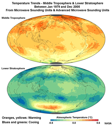
As more greenhouse gases accumulate in the atmosphere, climate models are projecting that the troposphere and surface could warm while the stratosphere above it cools.

Their predictions are being confirmed by satellite observations and shown in products like these. They were made from the Microwave Sounding Units and Advanced Microwave Sounding Units on several NOAA satellites flying since the late 1970s. The instruments detect microwave energy produced by atmospheric oxygen molecules and use that information to infer atmospheric temperature. Other microwave instruments continue the climate mission as well, such as the Advanced Microwave Sounding Units on EUMETSAT's Metop satellites and ATMS on the U.S.' NPP and future polar-orbiting satellites.

Both products were constructed from data collected between January 1979 and December 2005. The top image shows temperature trends in the middle troposphere centered around 5 km above the surface. Oranges and yellows indicate that the air in the lower half of the troposphere warmed significantly over most of the globe during this period. As you can see, the greatest heating occurred in the Arctic, while parts of the Antarctic cooled. The latter may be due to the ozone hole, which also cools the stratosphere.

The lower image shows temperatures in the lower stratosphere centered around 18 kilometers above the surface. Notice that the globe is largely dominated by blues and greens, indicating that the stratosphere cooled during this period. The warm areas over the Arctic and Antarctic are influenced by periodic events known as sudden stratospheric warmings. Continued satellite observation of the stratosphere will help scientists determine how significant these localized trends are and better understand the root causes.

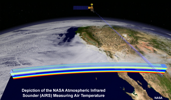
Infrared-based sounding instruments, such as the High-resolution Infrared Radiation Sounder or HIRS, also make important contributions to monitoring atmospheric temperature. While they can only profile the atmosphere in clear to partly cloudy sky conditions, they provide temperature profiles at higher horizontal and vertical resolutions than...

...those derived from microwave instruments. Since the advent of HIRS, other infrared and microwave instruments from various international satellite operators are being used together to help extend the observed global temperature record.

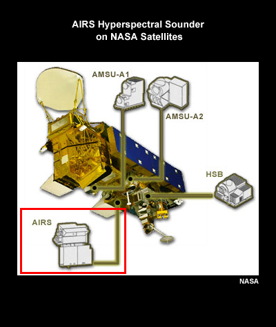
Advances in infrared sounding have also led to a new class of instruments, hyperspectral sounders, that let scientists profile the atmosphere in greater detail than ever before. Examples include NASA's AIRS,

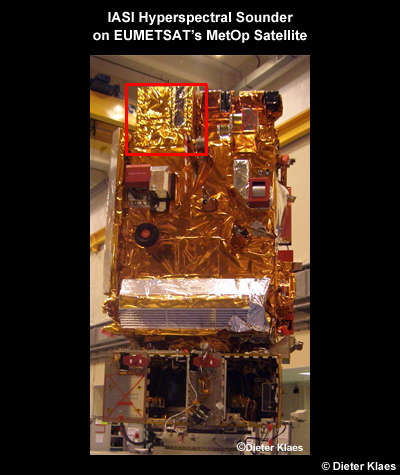
EUMETSAT's IASI,

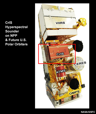
and CrIS on NPP and future U.S. polar orbiters.

Decadal to Long-Term Climate »
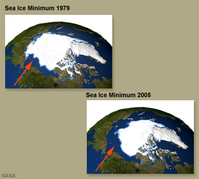
Sea Ice and Snow Cover

Observing changes in Earth's snow and ice cover is critical to understanding the impacts of the warming or cooling of Earth's atmosphere, land, and oceans. Scientists use observations of glaciers, ice caps, and ice sheets as a kind of thermometer for Earth's climate. The observations, in turn, help them project how these changes will impact us.

Given their global reach, satellites are perfectly positioned to help measure changes in sea ice cover. This will be critical for helping to regulate shipping and other industries in the short term and adapting to climate change in the coming decades.

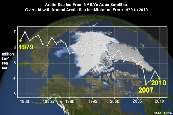
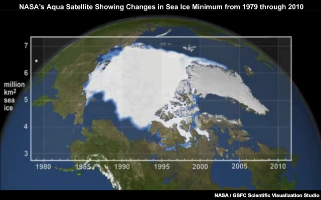
This image of northern Canada and the Arctic Ocean was taken by NASA's Aqua satellite in September 2010. As you can see, Arctic sea ice was near its minimum for the year. The previous month had the second lowest ice extent for any August on record (the lowest being in 2007).

Notice that the image appears to be cloud-free. That's because when Aqua's AMSR-E microwave sensor was operational, it observed microwave radiation emitted from the surface through cloud cover. Microwave radiation is emitted in much greater amounts by water than ice, letting us infer surface properties such as ice cover and ice age. This allows us to monitor sea ice year-round in spite of clouds and the long polar night.

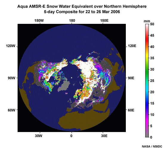
Satellite-based microwave instruments are also effective for monitoring snow cover and estimating snow water equivalent. This is crucial for monitoring snow melt and water storage.

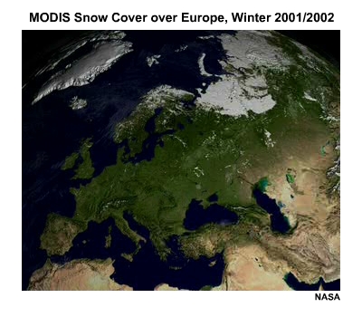
Satellite instruments that observe in the visible and infrared portions of the spectrum, such as the MODIS and NPP VIIRS imagers, also survey land-based snow cover over the entire planet each day. While their observations are impacted by cloud cover, their high resolution allows for more detailed snow mapping than is currently possible with microwave instruments.

For more information on sea ice and snow cover, see the COMET modules, Microwave Remote Sensing: Land and Ocean Surface Applications and Sea Ice and Products and Services of the National Ice Center.

Decadal to Long-Term Climate »
Sea Level Rise

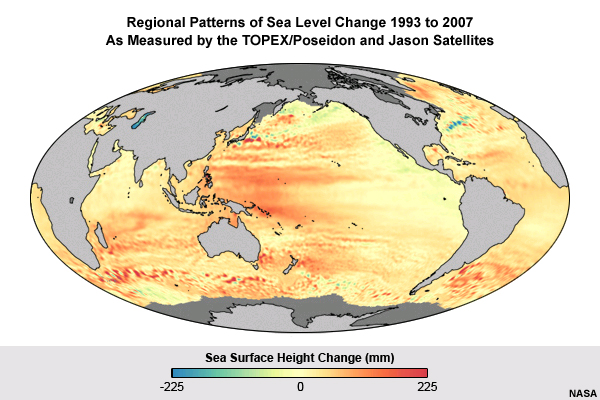
Sea level rise will soon become a problem for many low-lying areas but it will not be uniform. Some coasts will experience more of a rise than others. The thermal expansion of warmer sea water, added water from melting glaciers and ice sheets, salinity changes due to the influx of fresh water, and shifts in ocean currents can all affect local weather and climate conditions. Satellite instruments are very adept at measuring sea level height to supplement information from ocean and coastal buoys.

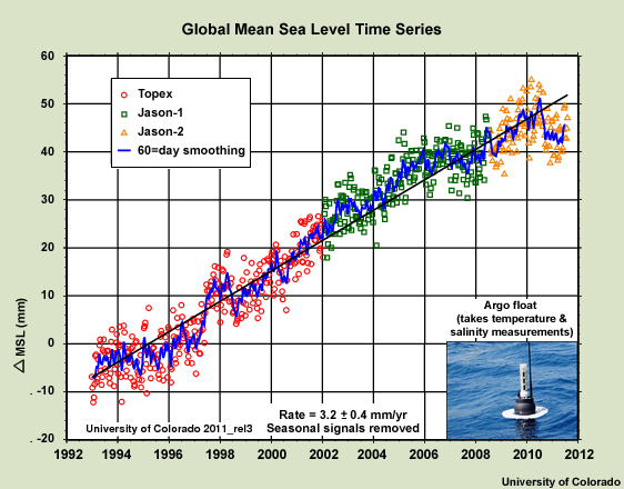
This graph shows over a decade's worth of data on mean sea level derived from the TOPEX/Poseidon and Jason-1 and-2 altimetry satellites. By combining data from altimeters with tide gauges and newly developed GPS buoys, scientists can now monitor sea level at the centimeter scale. The overall signal is clear. Since 1992, the world's oceans have gradually risen at a rate of about 3.2 millimeters per year. Scientists attribute half of this sea level rise to the thermal expansion of water as it warms, and the other half to melting land ice.

The continuous record of sea surface height that began with TOPEX/Poseidon in 1992 has been extended with Jason-2/OSTM (the Ocean Surface Topography Mission) in 2008. Without this continuity, information about the variation of ocean currents and heat stored in the oceans would have been lost and less would be known about climate variability.

Measurements from two other satellite missions, the Gravity Recovery and Climate Experiment or GRACE and the European Space Agency (ESA's) Gravity field and steady-state Ocean Circulation Explorer (GOCE), are helping to improve our understanding of the causes of sea level rise and for monitoring the thickness of ice sheets. GRACE is a joint mission between NASA and the German Aerospace Center or DLR.

For more information on sea level rise and its monitoring, see the COMET modules Coastal Climate Change and Jason-2: Using Satellite Altimetry to Monitor the Ocean.

Decadal to Long-Term Climate »
Trace Gases

Atmospheric trace gases constitute less than 1% of the volume of Earth's atmosphere. However, they are responsible for the greenhouse effect, which helps regulate our planet's temperature and is essential for life on Earth. Without a natural greenhouse effect, the temperature of Earth's surface would be about -18 degrees Celsius instead of its present 14 degrees Celsius. The current concern is not that we have a greenhouse effect, but that human activities are increasing it.

The trace gases that contribute to Earth’s greenhouse effect include water vapor, carbon dioxide, methane, nitrous oxides, sulfur dioxides, chlorofluorocarbons or CFCs, ozone, and other minor constituents. Not only do they absorb and emit thermal infrared radiation in the atmosphere; but when some are present in sufficient quantities near the surface, they are considered pollutants and can potentially harm human health. Examples include nitrous oxides, sulfur dioxides, and ozone.

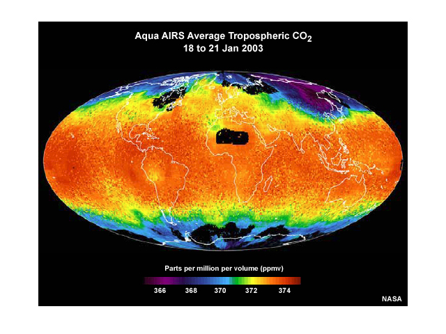
Concerns about Earth’s climate and the potential for climate change have increased the need for international observations of greenhouse gas emissions and climate monitoring on a global scale. Only satellite observations can deliver this type of global data. They help scientists define the distribution of greenhouse gases, quantify their sources and sinks, and monitor their transport. Satellites also help with assessing the relative importance of trace gases in chemical reactions throughout the atmosphere.

In addition to monitoring human activities that contribute to changes in trace gases, it's also important to monitor those from natural sources. These include nitrous oxides and methane emitted from soils and oceans, and sulfur dioxide emitted from volcanic eruptions.

Hyperspectral sounders show great promise for observing trace gases. This animation of sulfur dioxide plumes emitted from the Grímsvötn volcanic eruption from 21 to 24 May 2011 illustrates the extensive reach that a single event can have.

Follow-on missions, such as the CrIS hyperspectral sounder on NPP and future U.S. polar orbiters, and those planned by other countries, will extend the observation record and improve our understanding of the role of trace gases in Earth's greenhouse effect.

Decadal to Long-Term Climate »
Ozone, A Special Trace Gas

Satellite measurements of the concentrations and distribution of ozone in the atmosphere help scientists monitor climate cycles such as the QBO. Ozone also plays an important role as a greenhouse gas. In the stratosphere, it prevents most harmful UVB radiation from passing through the atmosphere. However, when it's present at greater amounts in the lower troposphere, it becomes a pollutant and is generally recognized as a health risk.

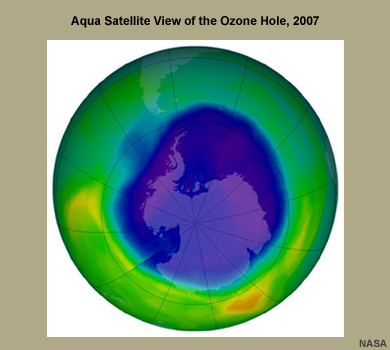
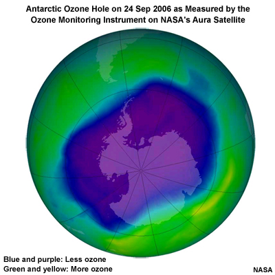
The depletion of stratospheric ozone became a growing concern in the late 1970s when satellite instruments such as TOMS provided the first confirmation of an ozone hole over the Antarctic.

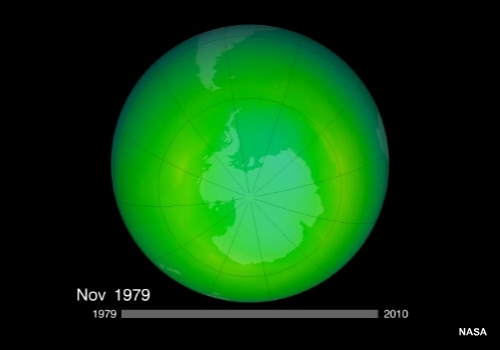
TOMS flew on a series of satellites from 1979 to 1999, measuring differences in total column ozone levels across the globe. It also began to document a global trend in ozone depletion at about 4% per decade.

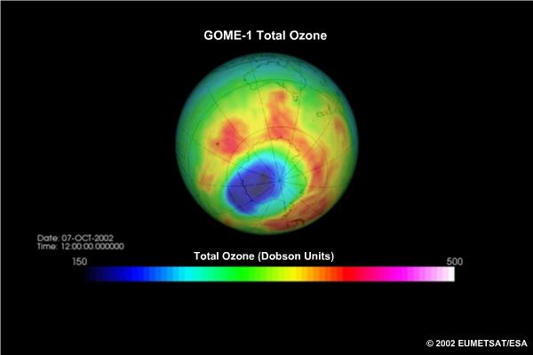
Since then, other satellite missions have extended the ozone data record. The first was GOME (the Global Ozone Monitoring Experiment) on Europe's ERS-2 satellite launched in 1995. Successive missions include:

• SCIAMACHY (SCanning Imaging Absorption SpectroMeter for Atmospheric Cartography) on Europe’s ENVISAT satellite (2002)
• OMI (Ozone Monitoring Instrument) on NASA’s EOS Aura satellite (2004), and
• GOME-2 on EUMETSAT’s Metop-A polar orbiter (2006)

Hyperspectral infrared sounders, such as AIRS and IASI, have started contributing to ozone monitoring. Together with measurements from dedicated ozone instruments such as OMI and GOME-2, ozone profiling products are now available. Most cover the lower stratosphere and upper troposphere where ozone concentrations are greatest and can vary significantly.

Metop and NPP polar orbiters are continuing the ozone monitoring mission. In addition to measuring total ozone content, OMPS (the U.S. Ozone Mapping and Profiler Suite) is capable of documenting the vertical structure of ozone from the stratosphere down into the troposphere with improved resolution and accuracy. When combined with the established ozone record, these newer measurements will shed additional light on how ozone is distributed, its sources and sinks, and how it's transported by the atmosphere.

Challenges for Satellite Monitoring »
Introduction

Scientists and decision makers need accurate, stable, and long-term climate data, like those obtained from satellites, to make decisions about the adaptation to and mitigation of climate change. Satellites provide:

• Opportunities for improving the short-range forecasting of severe weather and other atmospheric hazards
• Improved data for climate monitoring and input to numerical weather prediction
• Improved information for nearly all industries, from land use, ecology, disaster monitoring, and agricultural forecasting, to sea transport, fishing, and offshore industries to aviation, agriculture, engineering, construction, oil, gas, water, and electricity

Getting long-term climate data with sufficient accuracy and stability poses scientific, technical, and political challenges for satellite providers and operators. We'll explore these challenges in the rest of this section.

Challenges for Satellite Monitoring »
Scientific Challenges

Continuity

Satellites must operate on a continuous basis, without gaps between missions, to keep track of each climate related element and cycle. Otherwise, scientists may miss the onset of an event or the event altogether. For example, if a satellite measuring sea surface temperature is lost for several months, forecasters might miss the onset of an El Niño and end up unable to forecast it.

Satellites monitoring the ozone hole have seen it recover very gradually since 2000. But scientists aren't sure if there will be a full recovery or when it might happen. Without continuous monitoring of stratospheric ozone, they might miss a period in which the hole changes.

Continuous monitoring of each climate cycle is also critical for discerning the interactions between them and predicting their specific impacts.

Precision, Accuracy, and Stability

Highly accurate and stable data enable us to understand shorter-term processes and changes. But to estimate and monitor trends, data stability is the overriding concern. Climate scientists define it as the extent to which the accuracy of a time-averaged product remains constant over a long period, from years to decades. Even if a data set has a bias or is less than precise, the bias and level of precision need to remain the same over time.

Some measurements must also be made at the same time of day and location over the years. If a polar orbiter passes over a location at one o'clock in the afternoon rather than at noon, it will impact measurements that vary over the course of the day, such as sea surface temperature. This is less critical for measurements without distinct day-night cycles, such as concentrations of stratospheric ozone. Scientists can correct for the change in a satellite's orbit, but corrections are not ideal and orbital drift continues as polar orbiters age.

When new polar-orbiting satellites are launched, be it by the same country or a different one, the operators must ensure that orbits are coordinated so the observations occur at the right time. If a new satellite passes a fixed spot at 15 UTC instead of 12 UTC, its observations won't be comparable to the older ones and may not be as suitable for monitoring a particular longer-term climate cycle or trend.

Resolution

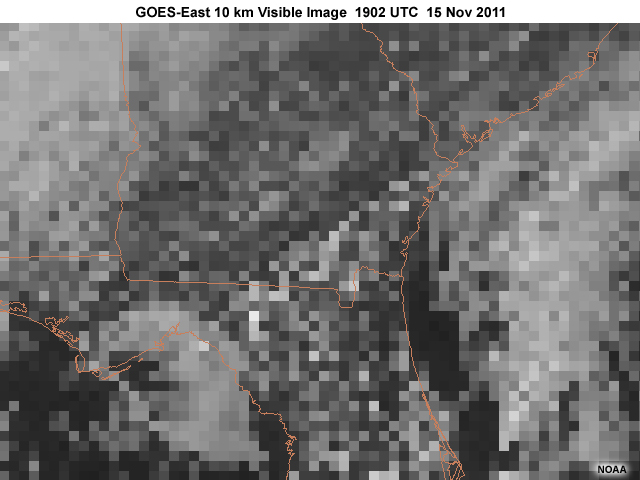
Spatial resolution is an important property related to precision. For example, satellites with 10-km resolution miss cumulus clouds that tend to be a few kilometers wide.

Even when satellite resolution is increased, numerical models may not be able to use the finer-scale data. For example, a newer satellite might observe clouds at 1-km resolution but a climate model might only accept 10-km resolution data. Modeling Earth's climate is complex, time consuming, and expensive, and it can take a while for the models to catch up to the observations.

Future Improvements

Scientists are working toward improved monitoring capabilities in several areas. For example, satellites tend to see the tops of clouds well. But they do not yet do a very good job of distinguishing all of the cloud layers in the atmosphere. Scientists would like to study cloud composition, size, and type in more detail, in part because cloud properties are becoming increasingly important elements of climate and weather prediction models.

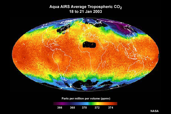
Scientists are also working to improve satellite monitoring of trace gases such as carbon dioxide, methane, and nitrous oxide, which are potent greenhouse gases. Scientists roughly know their concentrations in the atmosphere. But they need better spatial data to see exactly where the gases are being emitted, what their vertical distribution through the atmosphere is, and where and by how much they are being taken up by the planet.

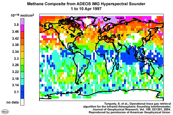
Scientists are also working to improve satellite monitoring of trace gases such as carbon dioxide, methane, and nitrous oxide, which are potent greenhouse gases. Scientists roughly know their concentrations in the atmosphere. But they need better spatial data to see exactly where the gases are being emitted, what their vertical distribution through the atmosphere is, and where and by how much they are being taken up by the planet.

In addition, scientists hope that ESA's Soil Moisture and Ocean Salinity monitoring mission (SMOS) and NASA's Aquarius mission will help them better understand and model ocean currents, and see how melting ice caps and glaciers might be affecting ocean circulation patterns and, by extension, climate.

Challenges for Satellite Monitoring »
Technical Challenges

Measuring climate variables with accuracy and stability over the long term are among the central challenges of using satellites to monitor climate. Long-term archives must be sustained and must include the actual data along with descriptive metadata about each observation and the complementary ground truth.

These archives need to be easily accessible and must have the capacity to reprocess complete satellite mission datasets when needed. Monitoring and archiving activities can be cost intensive but need to be sustained over the long term to be of use to climate monitoring.

As instruments age, their capabilities diminish. Just as a human eye may not see things as clearly or vividly as it ages, satellite sensors tend to lose their sensitivity and accuracy with time. The data values tend to drift and become noisier. But scientists know this and can at least partially account for the changes. For example, if an instrument makes things look colder than it used to, the observations can be calibrated so the data remain consistent.

Spacecraft operators routinely make these adjustments with guidance from scientists.

Satellite operators and scientists use many other techniques to ensure that measurements remain stable.

For example, they:

• Validate and analyze their data
• Scan the data for systematic errors and remove them
• Track and eliminate instrument biases
• Inter-calibrate identical instruments and compare similar instruments on different satellites
• Make sure that satellites collect data at regular intervals and over reliable periods of time
• Develop consistent and reliable processing algorithms

When a satellite changes, scientists must integrate new observations into the ongoing climate data record. The data may be completely usable, partially usable if adjustments or corrections are made, or may be completely useless for some climate monitoring applications. Building satellites with longer life spans can help. It reduces the need to compare and stitch together data from different satellites, generating better, more stable long-term data records. And overlaps between satellite missions with similar observing capabilities allow scientists and satellite operators to intercalibrate their measurements. When differences arise, the overlaps help them determine if they're related to design differences, problems with the sensors, or other factors that can be documented and possibly addressed.

Launching satellites that can maintain consistent equatorial crossing times and altitudes helps ensure that the measurements are taken at the desired time of day over the life expectancy of the spacecraft. The technical details of satellite orbits are routinely negotiated when the needs of climate modelers differ from weather forecasters. For example, the requirements for stable orbits have been met for almost all European polar-orbiting satellites and range between plus or minus two minutes.

New technology may help scientists with remaining challenges. For example, climate scientists need precipitation observations with better accuracy and spatial and temporal resolution. For now, they largely make indirect inferences to help fill gaps in the observations. But direct observations of precipitation size, type, duration, and location would be better. That could be accomplished with active radar upgrades to current passive satellite instruments, such as the one being planned for NASA's Global Precipitation Measurement (GPM) multi-satellite mission. A radar-observing capability will also help scientists detect and measure the content of cloud layers. Passive instruments see mainly cloud tops and integrated cloud properties while radar uses its penetrating microwave energy to peer into clouds.

Finally, climate scientists are hoping for better satellite-based atmospheric soundings (vertical profiles of temperature and moisture) with improved accuracy and global coverage. These will help solve the atmospheric portion of the climate puzzle since they will allow for much finer vertical slicing of atmospheric temperature and moisture. Hyperspectral sounding goes a long way towards meeting this goal and is already a reality for some polar-orbiting satellites.

Challenges for Satellite Monitoring »
International Coordination and Funding Challenges

Our planet is so large that it's nearly impossible for one country to monitor it. With dozens of satellites in orbit from various countries, coordination and cooperation are key to conserving resources, eliminating redundancy, and providing backup. Europe and the United States coordinate their polar-orbiting satellites with just such an aim in mind. And the Chinese, Brazilians, Indians, Japanese, Russians, and others also cooperate on satellite-related issues and resources.

Sometimes countries modify their orbits or provide extra instruments for other countries' satellites. Satellite operators from different countries also share technical knowledge, such as ideas for improving instruments and maximizing their performance.

The Global Climate Observation System (GCOS) was founded with cooperation in mind. GCOS provides principles and guidelines to satellite operators for acquiring and storing observations from satellites and other sources that are helpful for monitoring climate. In response, satellite operators have started several international activities to produce Climate Data Records (or CDRs). This includes the WMO SCOPE-CM initiative. (It stands for Sustained, Coordinated Processing of Environmental Satellite Data for Climate Monitoring.) GCOS also helps coordinate international satellite mission planning and tries to persuade countries to share their data with others.

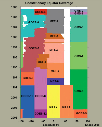
Finally, there are political challenges to that all-important factor for satellite monitoring: continuity. New governments may reduce funding for satellites, which can threaten the quality or even loss of climate monitoring variables. When this happens, other countries may be able to help fill the void. For example, in the late 1980s, the United States only had one geostationary satellite in orbit and could not cover both the Pacific and Atlantic Oceans. Europe had a spare, and moved it west to help with coverage until the U.S. could launch a replacement satellite. Much coordination and discussion had to take place before it could happen—but happen it did. It also made it easier for the U.S. to loan Japan a geostationary satellite to fill a gap in coverage between its launches. With such ongoing cooperation, satellites will continue monitoring the Earth and providing the data needed to increase our understanding of climate and make predictions that can improve and save people’s lives and help us plan for the future.