About the Lesson
This short lesson describes the Advanced Microwave Scanning Radiometer 2 (AMSR2) on board the next-generation polar-orbiting satellite platforms. AMSR2’s primary mission is to improve scientists’ understanding of climate by providing estimates of precipitation, water vapor, cloud water, wind velocity, sea surface temperature, sea ice concentration, snow depth, and soil moisture. AMSR2 also advances weather forecasting through real-time imagery, value-added products, and input to numerical weather prediction. This lesson is part of the Satellite Foundational Course for JPSS (SatFC-J).
On completing the lesson, you should be able to:
- Describe the capabilities of the AMSR2 microwave imager onboard the GCOM-W polar orbiters
- State swath width and spatial resolution
- Describe the AMSR2 spectral bands/channels and their main applications
- Identify key environmental product areas to which AMSR2 observations contribute
Introduction
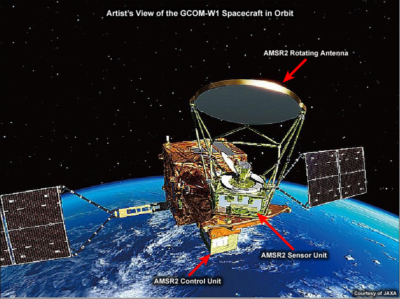
Through a partnership with the Japan Aerospace Meteorological Agency(JAXA) and NOAA, the Joint Polar Satellite System (JPSS) obtains timely access to Advanced Microwave Scanning Radiometer 2 (AMSR2) data. AMSR2 is carried on board JAXA’s GCOM-W1 (Global Change Observation Mission, first mission) polar-orbiting satellite. Launched in 2012, GCOM has a life expectancy likely to extend to 2018 and beyond. The AMSR2 imager is a nearly identical follow-on to the previous AMSR-E imager that operated until 2011 on NASA’s Aqua satellite.
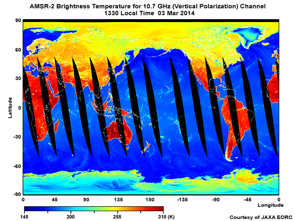
AMSR2 produces two-dimensional imagery of brightness temperatures and a variety of derived geophysical products useful to analysts and forecasters. To learn more about JPSS microwave sounders which produce three dimensional temperature, pressure, and moisture profiles, see the SatFC-J lesson, The CrIS and ATMS Sounders.
AMSR2’s primary mission is to improve our understanding of climate. Towards that end, measurements are used to calculate the atmospheric fields of precipitation, water vapor, cloud water, and wind velocity near Earth’s surface, and the surface fields of sea surface temperature or SST, sea ice concentration, snow depth, and soil moisture. In addition to its climate focus, AMSR2 advances weather forecasting through real-time forecaster imagery, value-added products and input to numerical weather prediction.
Orbit
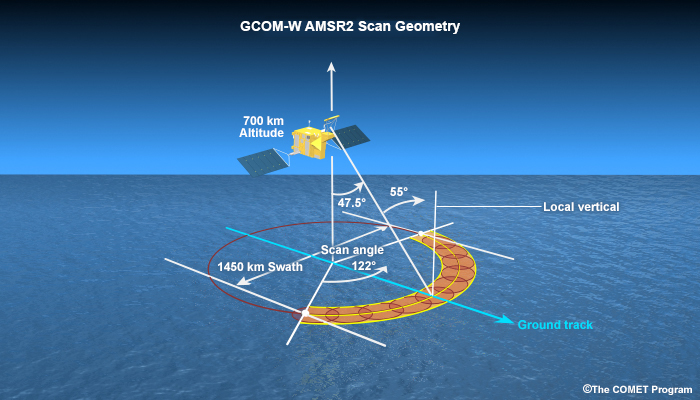
GCOM-W1 flies in a polar orbit at an altitude of 700 km. It crosses the equator at 0130 and 1330 local time and produces swaths of 1450 km. There are gaps near the equator but overlap toward the poles.
The GCOM-W1 polar orbiter has almost the same crossing time as the JPSS constellation’s Suomi NPP and JPSS satellites that cover the early afternoon orbit. NOAA’s POES (Polar Operational Environmental Satellites) constellation of weather satellites also includes a partnership with EUMETSAT and their Metop satellites that cover the mid-morning 0930 orbit, and the Air Force’s DMSP (Defense Meteorological Satellite Program) polar orbiters that fly in an early morning orbit around 0530 local time. It’s worth noting that current DMSP satellites also have microwave imagers similar to GCOM’s AMSR2.
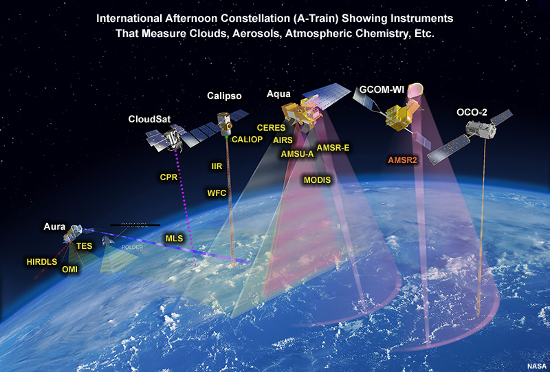
Additional satellites from NASA’s “A-train” constellation have nearly the same early afternoon orbits as GCOM-W1 and S-NPP/JPSS, allowing near simultaneous observation of a wide variety of phenomena. That leads to better science and improved weather forecasting.
Scan Strategy
AMSR2 uses a conical scan strategy, imaging data points in an arc that sweeps in front of the satellite as it moves forward. This produces a 55-degree incidence angle with Earth’s surface, allowing measurements at vertical (V) and horizontal (H) polarizations at each frequency measured. This “dual polarization” offers the capacity to make important corrections to measurements, something not possible with more standard scan strategies.
Channel Frequency and Footprint Size
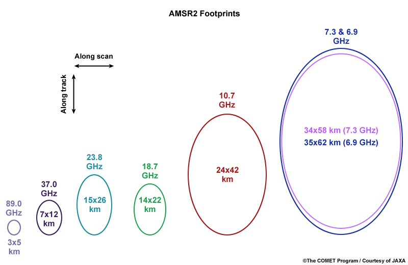
The amount of microwave energy emitted by Earth’s surface and atmosphere is several orders of magnitude less than in the infrared region. This requires microwave sensors to employ larger fields of view than traditional visible and infrared sensors. As microwave frequency decreases (wavelengths get longer), emitted energy continues to decrease, and progressively larger footprints, with minor exceptions, are needed to collect enough energy for imagery and derived products.
At the highest frequency (89 GHz), the footprint size is about 3 by 5 km. This is sufficient for high-resolution imagery for forecasters. At the lowest frequencies (6.9 and 7.3 GHz), footprints are much larger and imagery is less useful. Data at these frequencies is generally used in derived products.
Compare the coarseness of the 6.9 GHz image with its large imaging footprint to the sharpness and detail of the 89 GHz image with its much smaller footprint. The 89 GHz channel is also more sensitive to atmospheric gases, clouds and precipitation. Notice the cloud bands in the 89 GHz image compared to the 6.9 GHz image.


Environmental Parameters
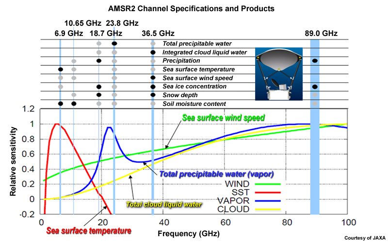
By combining channels, retrieval algorithms produce a diverse set of environmental parameters. The black shaded circles in the upper part of the graphic show the key input channels for the parameters.
The lower panel of the graphic shows the relative sensitivity of selected geophysical parameters. For example, sea surface temperature can only be assessed by the lowest frequencies, while sea surface wind speed can be sensed over the full spectral range. Notice how Total Precipitable Water depends on the water vapor absorption region centered near 23 GHz. Derived sea surface temperature, surface ocean wind speed, and soil moisture are among the parameters that benefit the most from the expansive range of sensing frequencies. AMSR2 can observe surface phenomena in nearly “all weather” conditions.
Imagery Interpretation
In general for forecasting applications, the horizontal polarization image is better to view than the vertical polarization image because it conveys maximum contrast between the ocean surface vs. clouds and precipitation. The two most valuable kinds of imagery for forecasters come from 36.5 and 89.0 GHz. They have the highest spatial resolution, can penetrate most cloud cover allowing for observation of surface features in the vast majority of weather conditions, and can probe the interior of clouds to reveal information about microphysics and precipitation.
Drag the slider to compare AMSR2 36.5 and 89 GHz horizontal polarization images for tropical storm Ophelia.
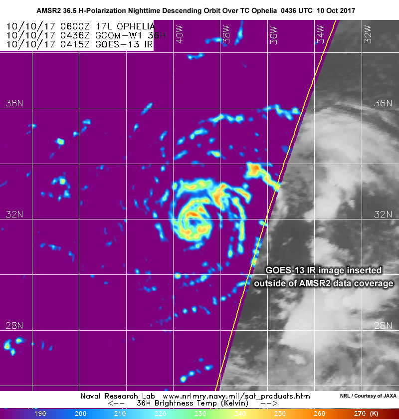
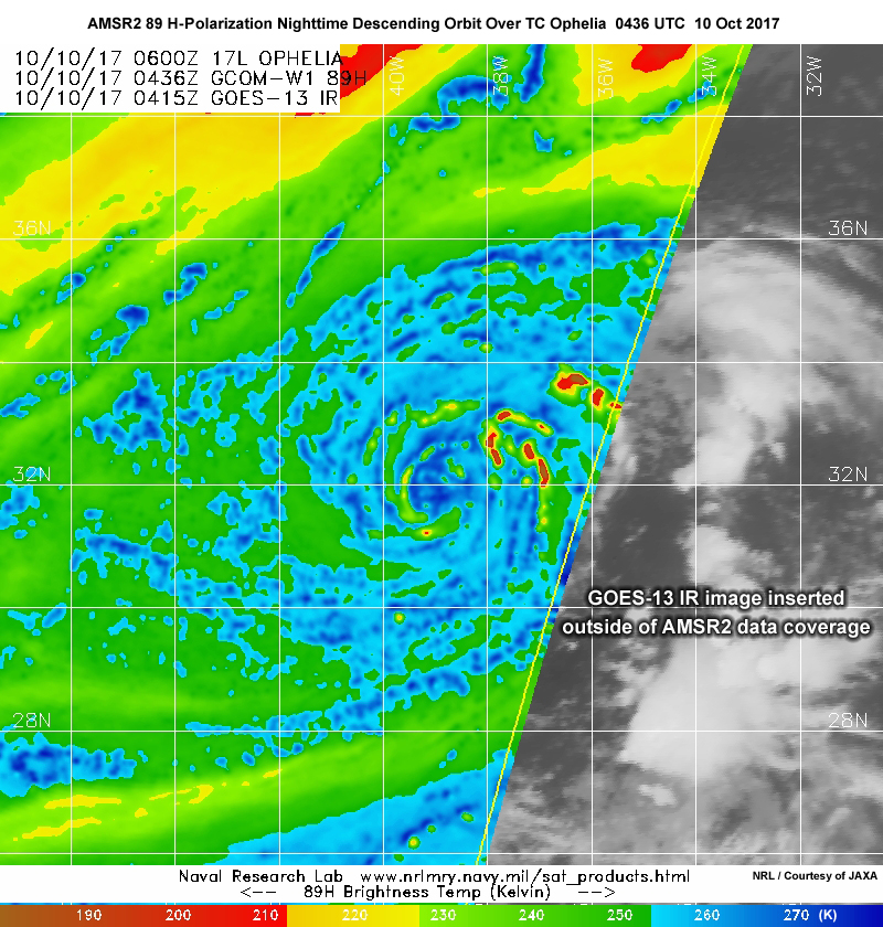
AMSR2 36.5 and 89 GHz images (both horizontal polarization) for tropical storm Ophelia in the North Atlantic. The 36.5 GHz image emphasizes moderate to large water droplets whereas the 89 GHz image emphasizes smaller water droplets and also ice hydrometeors within deep convective clouds.
Using microwave images of raw brightness temperatures for forecasting can be challenging. Fortunately, over tropical oceans, it’s relatively straightforward to infer the structure of tropical cyclones and convection systems from the H polarization. Over midlatitude oceans and polar seas however, interpretation is often not straightforward since the radiometrically cold sea surface tends to resemble either cloud or precipitation signatures.
Here’s an example of this ambiguity over TC Gert which is undergoing midlatitude transition.
Drag the slider to compare AMSR2 89 GHz and GOES-13 longwave IR images taken within 20 minutes of each other.
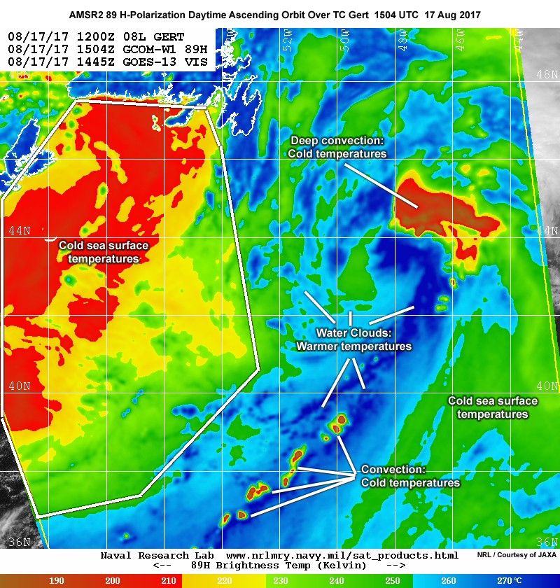
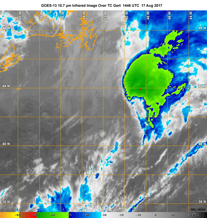
In the 89 GHz (horizontal polarization) image, notice that cloud-free calm waters, on one hand, and deep convection, on the other, both appear cold (mainly reds and yellows). It can be difficult telling one feature from the other. Low clouds and raining stratiform clouds produce higher temperatures (blues and greens) as does a wind roughened ocean surface. These can be observed around the circulation of tropical cyclone Gert.
For more information on microwave emission and polarization at the different frequencies, see the companion SatFC-J lesson, Introduction to Microwave Remote Sensing. For additional more in-depth information on microwave land, ocean, and atmospheric remote sensing for various applications, see the COMET distance learning course titled, Microwave Remote Sensing Topics Distance Learning Course.
Nowcasting Tropical Cyclones
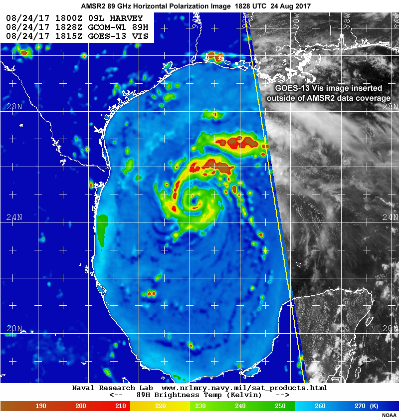
Real-time microwave brightness temperature images of tropical cyclones deliver critical information to forecasters about storm structure and intensity. Among today’s microwave instruments, AMSR2 provides some of the highest resolution images for this purpose. This GOES-16 longwave infrared image is showing an intensifying Hurricane Harvey approaching the Texas coast. It shows a Category 1 storm, barely a minimum hurricane with maximum sustained winds of 75 knots. The storm has an eye at this stage, but it’s not completely discernible on this image. Notice that cirrus cover a good portion of the northwestern Gulf of Mexico.
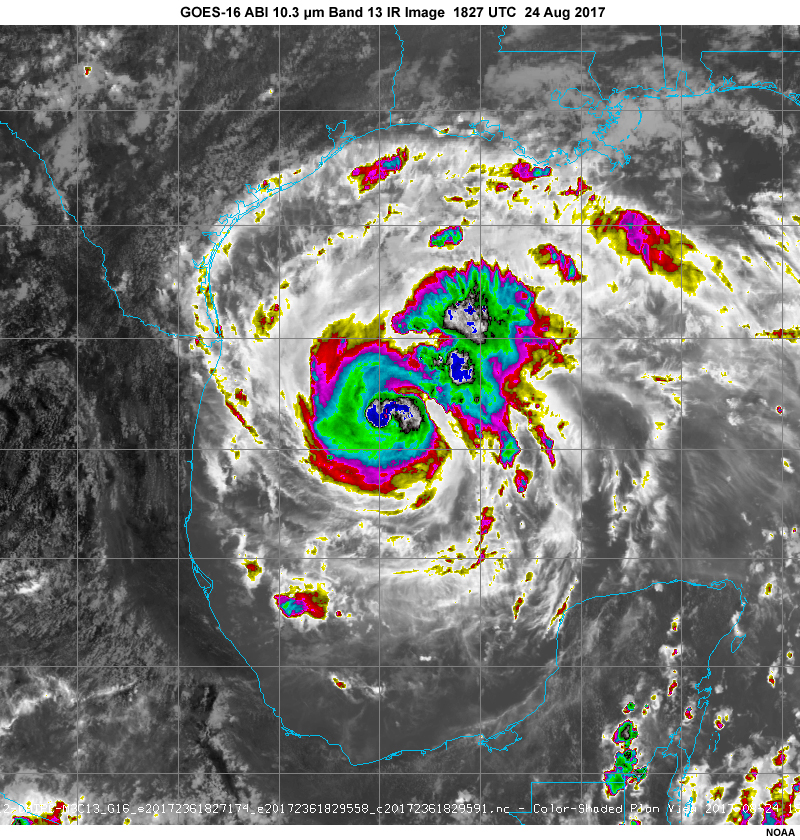
Now let’s examine the AMSR2 89 GHz image taken at the same time. Insensitive to thick cirrus which affected the GOES-16 infrared image, the microwave image shows heavy precipitation in reds, yellows and greens. It resembles an image from a ground-based weather radar. Notice the rainbands and the storm’s eye are easily identified. Polar-orbiting satellites provide less frequent refresh than geostationary imagers. But if enough polar microwave imagers are orbiting at once, then periodic images will still be available to compliment geostationary images.
Atmospheric Rivers
Landfalling atmospheric rivers of low-level moisture can produce heavy precipitation over concentrated regions. But they’re often difficult to nowcast. Geostationary water vapor images show cirrus and upper-level water vapor but not the low-level, high-dewpoint air masses that carry the bulk of the moisture in these rivers. Images of total precipitable water derived from microwave imagers give forecasters quantitative information. Since water vapor in the lowest kilometer or so is the primary contributor to TPW, it is an excellent tool for tracking atmospheric rivers.
This TPW product composite over the eastern Pacific combines several passes of passive microwave data, including AMSR2. Abundant tropical water vapor (in reds) appears in the subtropics. Lesser amounts (in blues) approach the California coast, powered by a strong jet stream. The brighter band off the central California coast is an atmospheric river that brought heavy rain to the California central coast. When composites like this are animated, they provide remarkable depictions of the evolution of atmospheric rivers and landfall.
To view realtime images and animations of the CIMSS MIMIC-TPW hourly product, go to the CIMSS web page at MIMIC-TPW.
Arctic Ice
Microwave channels penetrate cloud cover, which blocks other satellite sensors from observing sea ice. The data are useful even during the long polar nights when solar, reflected light channels from other satellites are useless.
This animation is based on AMSR2 89 GHz data. Land and sea backgrounds are incorporated from independent sources for context, including NASA’s Blue Marble Next Generation database. As navigation increases in the Arctic, depictions like this will be crucial for timely warnings of sudden ice sheet growth, melt and movement.
This animation shows the Earth rotating as Arctic sea ice advances from 25 Feb 2015 to 11 Sep 2015 when it reached its annual minimum extent.
Sea Surface Temperature
AMSR2 generates sea surface temperature through clouds except in heavy rain conditions. Infrared SSTs are available more frequently and at higher spatial resolution but are often contaminated by clouds. Research has shown that the two sources can fill in each other’s gaps, producing a seamless and continuously available product. Implementing this synthesis into operations promises to boost the quality and timeliness of SST measurements.
AMSR2 has a key role monitoring SST shifts in the Pacific Ocean. This SST anomaly product shows the difference between the current AMSR2 SST and a background climatology. The elongated blue feature along the equator represents the cooler than normal waters of La Niña.

Two years of AMSR-E observations demonstrates the capacity of AMSR2 to observe seasonal changes in SST over the western hemisphere. In this animation, notice the Gulf Stream meandering off the east coast of North American as it moves toward Europe. The waters off the west coast north of Mexico stay relatively cool (blue) all year around. During winter, northeasterly offshore winds over southern Mexico produce occasional regions of cool water just off the west coast due to the upwelling of cooler waters from below. Upwelling also occurs off the west coast of South America, keeping waters generally cool all year around.
Summary
- AMSR2 flies on JAXA’s GCOM-W1 satellite; both JAXA and NOAA get real time access to the data
- GCOM-W1 flies in a polar orbit at an altitude of 700 km; it crosses the equator at 0130 and 1330 local time and produces swaths of 1450 km
- AMSR2 measurements are used to calculate and/or forecast precipitation, water vapor, cloud water, wind velocity near Earth’s surface, SST, sea ice concentration, snow depth, and soil moisture
- AMSR2 advances weather forecasting by providing real-time forecaster imagery, value-added products, and input to NWP
- AMSR2 uses a conical scan strategy, producing a 55-degree incidence angle with Earth’s surface; this allows measurements at vertical (V) and horizontal (H) polarizations at each frequency measured
- AMSR2 channels are much less sensitive to clouds and atmospheric effects than IR and VIS sensors. Its channels operate within atmospheric windows, except for 23.8 GHz, which operates within a water vapor absorption region
- The amount of microwave energy received by instrument varies directly with frequency so the footprint sizes required for adequate collection also vary. The footprint size at the highest frequency (89 GHz) is 5x3 km, and much larger at the lowest frequencies (6.9 and 7.3 GHz). This makes the higher frequency imagery suitable for forecasting, and the lower frequency imagery suitable for derived products
- Different geophysical parameters are assessed by different frequencies; for example, SST is assessed by the lowest frequencies while sea surface wind speed is sensed over the full spectral range; the AMSR2 23.8 GHz frequency has a special function to sense water vapor
- AMSR2 images provide useful information about the storm structure and intensity of tropical cyclones; are used to produce TPW products that help track atmospheric rivers; can monitor polar regions regardless of cloud cover or daylight; and can generate SST through clouds except in areas of heavy rainfall
You have reached the end of the lesson. Please complete the quiz and share your feedback with us via the user survey.
Resources
Internet Resources
Brief overview of GCOM-W1
https://en.wikipedia.org/wiki/Global_Change_Observation_Mission
Summary of AMSR2 from WMO
https://www.wmo-sat.info/oscar/instruments/view/28
Earth Observing Resources Detailed Description
https://directory.eoportal.org/web/eoportal/satellite-missions/g/gcom
GCOM-W1 and AMSR2 Description from JAXA
http://suzaku.eorc.jaxa.jp/GCOM_W/w_amsr2/whats_amsr2.html
El Niño Watch using AMSR2 data
http://sharaku.eorc.jaxa.jp/cgi-bin/amsr/elni/elni.cgi?lang=e
NOAA NESDIS Global Data Composites (near real time)
http://manati.star.nesdis.noaa.gov/gcom/datasets/GCOM2Data.php
NOAA NESDIS Powerpoint on AMSR2 Applications Development
http://www.data.jma.go.jp/mscweb/en/aomsuc6_data/oral/s09-03.pdf
Portals for Microwave Imagery of Tropical Cyclones
http://www.nrlmry.navy.mil/tc_pages/tc_home.html
https://www.fnmoc.navy.mil/tcweb/cgi-bin/tc_home.cgi
http://sharaku.eorc.jaxa.jp/TYPHOON_RT/
TPW Imagery
http://tropic.ssec.wisc.edu/real-time/mimic-tpw/natl/main.html
TPW over Tropical Cyclones
http://tropic.ssec.wisc.edu/
COMET Modules
- Using Microwave Images to View Tropical Cyclones
https://www.meted.ucar.edu/training_module.php?id=159 - Background about Satellite Microwave Sensors and Applications
https://www.meted.ucar.edu/training_module.php?id=260
Contributors
COMET Sponsors
MetEd and the COMET® Program are a part of the University Corporation for Atmospheric Research's (UCAR's) Community Programs (UCP) and are sponsored by NOAA's National Weather Service (NWS), with additional funding by:
- Bureau of Meteorology of Australia (BoM)
- Bureau of Reclamation, United States Department of the Interior
- European Organisation for the Exploitation of Meteorological Satellites (EUMETSAT)
- Meteorological Service of Canada (MSC)
- NOAA's National Environmental Satellite, Data and Information Service (NESDIS)
- NOAA's National Geodetic Survey (NGS)
- Naval Meteorology and Oceanography Command (NMOC)
- U.S. Army Corps of Engineers (USACE)
To learn more about us, please visit the COMET website.
Project Contributors
Program Manager
- Amy Stevermer — UCAR/COMET
Project Lead and Meteorologist
- Patrick Dills — UCAR/COMET
Science Advisors
- Tom Lee — UCAR/COMET
- Patrick Dills — UCAR/COMET
Graphics/Animations
- Steve Deyo — UCAR/COMET
Multimedia Authoring/Interface Design
- Gary Pacheco — UCAR/COMET
Audio/Video Editing/Production
- Dolores Kiessling — UCAR/COMET
- Gary Pacheco — UCAR/COMET
- Sylvia Quesada — UCAR/COMET
Narration
- Dolores Kiessling — UCAR/COMET
COMET Staff, February 2018
Director's Office
- Dr. Elizabeth Mulvihill Page, Director
- Tim Alberta, Assistant Director Operations and IT
- Paul Kucera, Assistant Director International Programs
Business Administration
- Lorrie Alberta, Administrator
- Auliya McCauley-Hartner, Administrative Assistant
- Tara Torres, Program Coordinator
IT Services
- Bob Bubon, Systems Administrator
- Joshua Hepp, Student Assistant
- Joey Rener, Software Engineer
- Malte Winkler, Software Engineer
Instructional Services
- Dr. Alan Bol, Scientist/Instructional Designer
- Tsvetomir Ross-Lazarov, Instructional Designer
International Programs
- Rosario Alfaro Ocampo, Translator/Meteorologist
- Bruce Muller, Project Manager
- David Russi, Translations Coordinator
- Martin Steinson, Project Manager
Production and Media Services
- Steve Deyo, Graphic and 3D Designer
- Dolores Kiessling, Software Engineer
- Gary Pacheco, Web Designer and Developer
- Sylvia Quesada, Production Assistant
Science Group
- Dr. William Bua, Meteorologist
- Patrick Dills, Meteorologist
- Bryan Guarente, Instructional Designer/Meteorologist
- Matthew Kelsch, Hydrometeorologist
- Erin Regan, Student Assistant
- Andrea Smith, Meteorologist
- Amy Stevermer, Meteorologist
- Vanessa Vincente, Meteorologist