About the Lesson

This lesson introduces you to the two visible imaging bands and one of the near-infrared bands on the GOES R-U ABI (Advanced Baseline Imager), focusing on their spectral characteristics and how they affect what each band observes. The near-infrared band at 0.86 micrometers is included because of it's close spectral proximity to the visible bands and complementary observing capabilities. Also included is a brief discussion of the customization of visible enhancements as an important consideration for improving the depiction of various features of interest.

On completing the lesson, you should be able to:

• Identify the ABI's two visible spectral bands, the "blue" and "red" bands, and various phenomena that can be detected in the spectral regions they cover
• Identify one of the ABI's four near-IR spectral bands, also known as the "veggie" band, and describe how it contrasts to the two visible spectral bands
• Identify sun glint in visible and near-IR imagery
• Identify favored times for viewing haze, dust and smoke, and which of the visible and near-IR bands is generally more sensitive to atmospheric aerosol detection
• Briefly state the advantage of adjusting enhancement tables in visible imagery for feature identification

Please note that this lesson was originally published prior to the launch of GOES-16 and used imagery from the Himawari-8 geostationary satellite to illustrate GOES-R ABI capabilities. The Himawari-8 imager, the AHI (Advanced Himawari Imager), has bands nearly identical to the ABI on board the GOES R-U series. In the interest of time, some of the original Himawari-8 imagery is still included where geographical context is not critical for understanding the concept.

Introduction

The Advanced Baseline Imager’s (ABI) two visible bands also known as the "blue" and "red" bands, and the near-IR band also known as the "veggie" band, are in the region of the electromagnetic spectrum where the sun emits most of its energy. That incoming energy is attenuated by molecules, clouds, and aerosols.

 

 

 

 

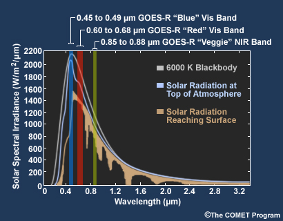
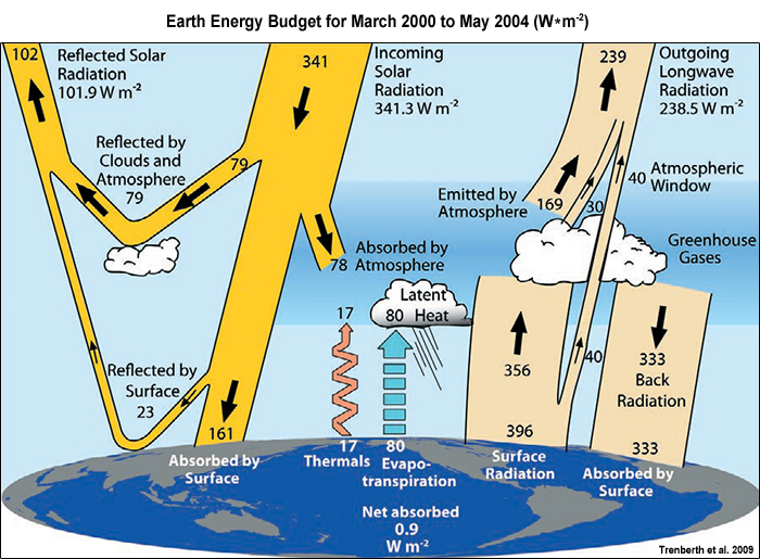
About 30% of the incoming energy is reflected by clouds, atmosphere and the surface, and another 23% is absorbed by the atmosphere and re-emitted to space. The remaining energy reaches the earth's surface where it is absorbed and re-emitted.

GOES-R+ ABI Visible and Near-IR Bands: Land and Water

The two graphs show albedos or reflectances, for clouds, water, snow cover, soil, and different types of vegetation. Reflection from soil and vegetation increases with wavelength, with a marked jump around 0.7 micrometers, especially for green vegetation since chlorophyll no longer absorbs solar radiation beyond the visible. Clouds and snow cover are highly reflective throughout the visible and into the "veggie" band portion of the near-infrared. And notice that water is poorly reflective, with almost no reflection beyond 0.9 micrometers.

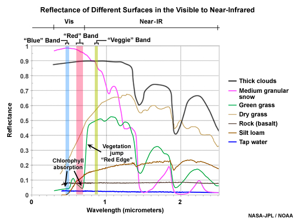
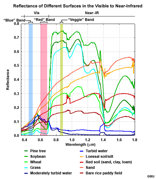
Highlighting the two GOES-R+ ABI "blue" and "red" visible bands, we see that their spectral coverages do not extend into the spectral range where vegetated surfaces become more reflective. The 0.86 micrometer band, or “veggie” band shown in green, is engineered for characterizing vegetated surfaces.

Another point worth noting is that the ABI's 0.64 µm "red" band, appears similar to legacy GOES 0.63 µm visible imagery due to their similar spectral coverages. The ABI's "red" band spatial resolution however is greater by a factor of two (0.5 km) when compared to legacy GOES visible imagery (at 1 km).

 

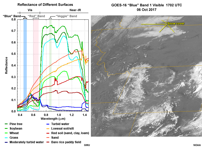
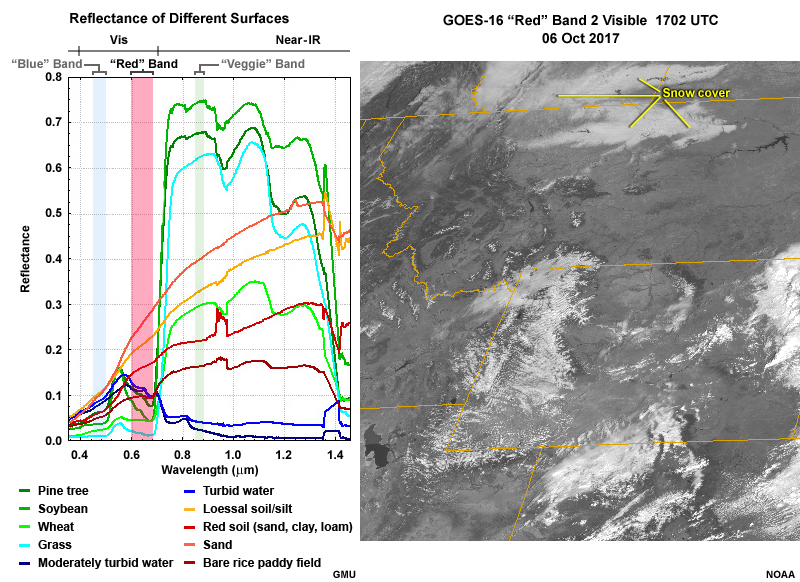
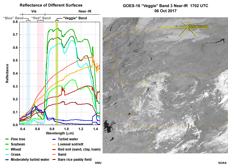
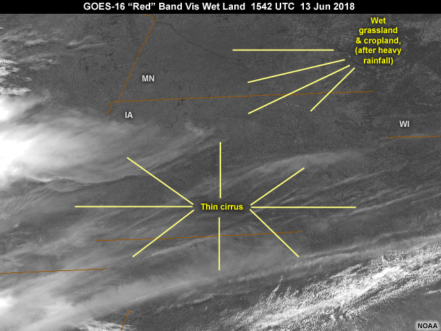
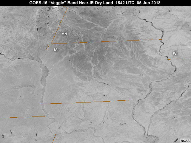
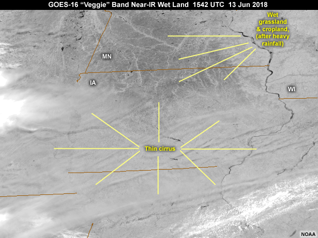
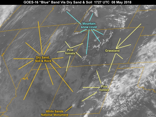
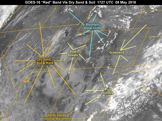
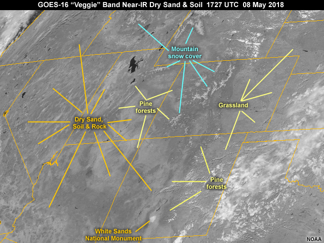
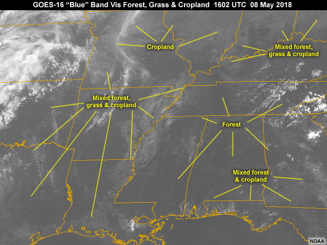
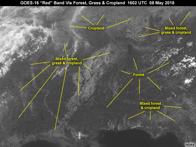
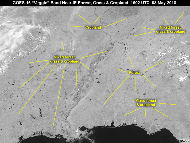
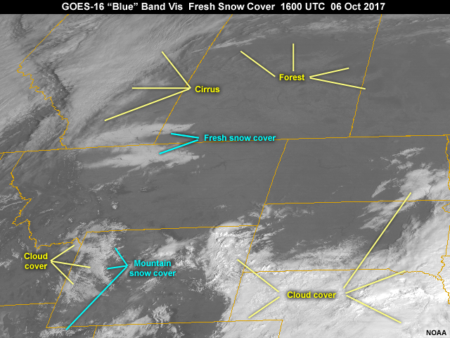
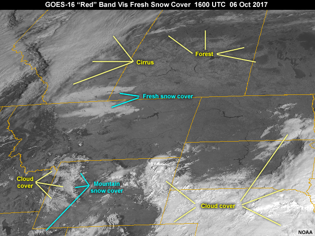
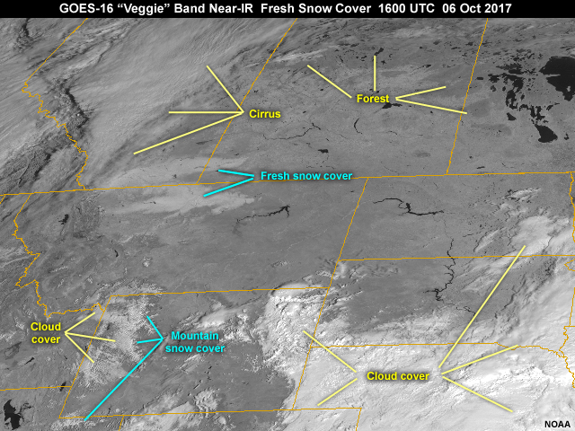
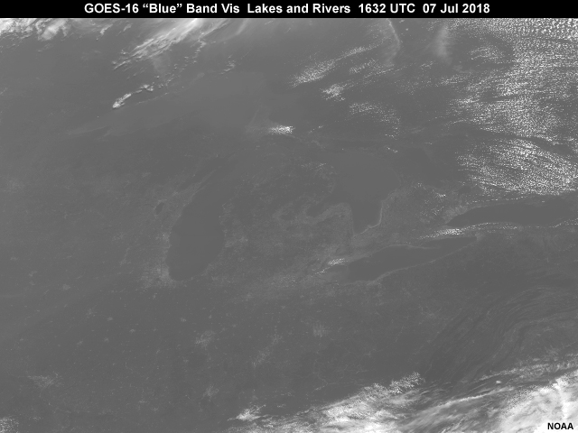
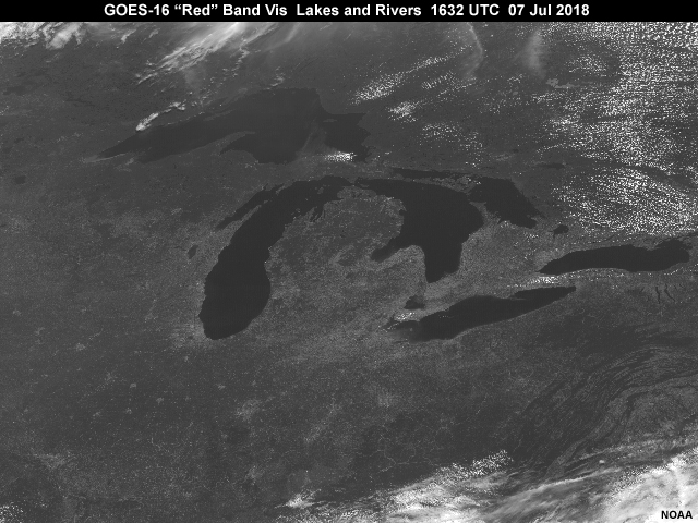
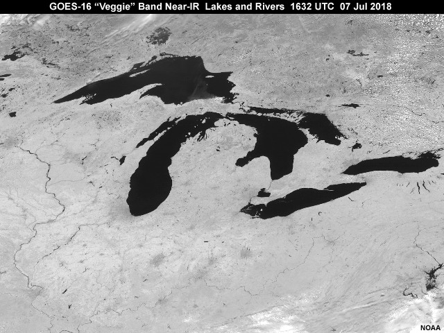
The GOES-16 "blue", "red", and "veggie" band images were taken over portions of the Northern Rockies and Northern High Plains during early October, and help confirm some of the main features seen in the reflectance curves.

Notice in all three bands that land surfaces appear brighter overall when compared to water surfaces. In the two visible bands, bare soil particularly when dry, appears even brighter than a vegetated or forest covered surface. In the "veggie" band however, the reverse is true where vegetated surfaces are more reflective compared to most bare land and especially water. The "veggie" band's sharp contrast between land and water makes it the preferred band for discriminating land from water.

For detecting cloud cover in the "veggie" band however, the brighter vegetation makes discrimination between vegetated surfaces and especially thinner or patchy cloud cover more difficult. The images show us that the "red" band with its darker surfaces is the best of the three bands for monitoring clouds.

It’s also evident that the brightness contrast between bare land and vegetative surfaces is more prominent in the "red" and "veggie" bands. Part of the reason for this is validated by the reflectance curves that show a bigger spread between land and vegetation surface types in these two bands when compared to the “blue” band. This enhanced sensitivity to vegetation allows the "red" and "veggie" bands to be used to calculate a normalized difference vegetation index (or NDVI) for monitoring vegetation health or "greenness".

Another factor reducing surface contrast in the "blue" band relates to the somewhat hazy appearance seen in the imagery. This is due to increased scattering of sunlight by small atmospheric aerosols like haze, dust, and pollutants, which become more prominent at shorter visible wavelengths and at least partially mask surface features.

We also see that some features, smaller cloud elements for example, appear sharper in the "red" band than in the other two bands. This is due to the "red" band's higher 0.5 km resolution compared to 1.0 km for the "blue" and "veggie" bands.

Taking these factors into account, it’s clear that the “red” and "veggie" bands are superior for highlighting and delineating surface properties.

 

Another aspect of the “red” visible band worth noting is that turbid water is detectable as relatively bright when compared to clearer, undisturbed, and deeper water conditions. Increases in turbidity usually follow meteorological episodes such as strong flow across coastal zones or heavy rains and resultant runoff into rivers and lakes.

Reflectance of Different Surfaces

This table compares the solar reflectance of different surface types for the three bands presented in this lesson. In the image comparisons, notice that the “red” visible band is usually more sensitive to land surface variations whereas the "veggie" near-IR band tends to place more emphasis on land vs. water differences. Also recall that "red" band images are taken at a higher 0.5 km resolution and will appear slightly sharper when compared to the 1-km "blue" and "veggie" bands.

Reflectance of Various Surfaces in the Spectral Range of Solar Radiation (0.38 to 0.90 micrometers)
Surface Type Reflectance (%) 0.38-0.70 µm Vis 0.86 µm Near-IR	Image Examples
Wet Soil Vis: 3-25 % NIR: 8-20 %	Before vs. After Rainfall Conditions Use the slider to compare images 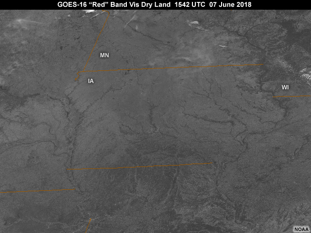0.64 µm "Red" Band Comparison 0.86 µm "Veggie" Band Comparison
Dry Soil Vis: 5-30 % NIR: 15-35 %
Dry Sand Vis: 5-30 % NIR: 35-45 %	"Blue" Vis Band "Red" Vis Band "Veggie" Near-IR Band
Grass Vis: 2-45 % NIR: 45-65 %	"Blue" Vis Band "Red" Vis Band "Veggie" Near-IR Band
Forest Vis: 5-20 % NIR: 20-55 %
Snow Cover (clean, dry) Vis: 75-98 % NIR: 50-95 %	"Blue" Vis Band "Red" Vis Band "Veggie" Near-IR Band
Snow (wet, dirty) Vis: 25-75 % NIR: 35-65 %
Water Surface (sun angle >25°) Vis: <10 % NIR: <5 %	"Blue" Vis Band "Red" Vis Band "Veggie" Near-IR Band
Water Surface (low sun angle) Vis & NIR: large range	"Blue" Vis Band "Red" Vis Band "Veggie" Near-IR Band

 

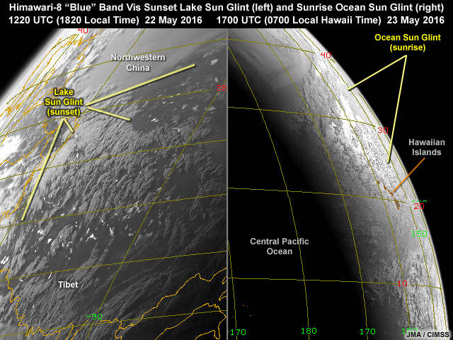
Sun Glint Over Water

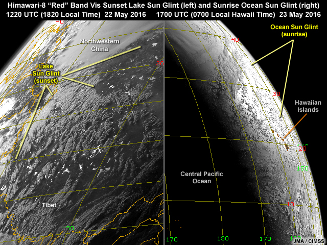
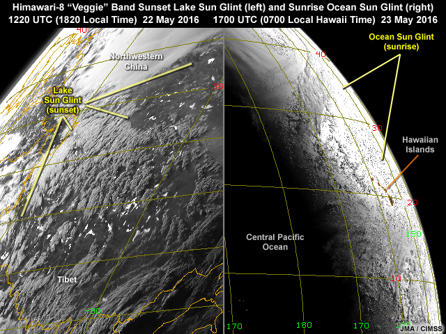
Sun glint is an important phenomenon that must be considered when viewing visible and near-IR images over water. When water surfaces are smooth, large reflections occur when the sun and satellite are properly aligned. In the loops, notice the bright region that moves from east to west as the sun moves. Also notice that the sun glint becomes more noticeable at longer wavelengths as the atmosphere scatters less sunlight and water surfaces become less reflective in areas not affected by sun glint.

Zooming into the South China Sea and Bay of Bengal regions reveals dark areas within the larger glint pattern of the sun that turn brighter with time as the sun-satellite geometry changes. These areas indicate relatively calm waters. As with a mirror, we don’t see an object’s reflection, in this case the sun, unless the sun-Earth and Earth-satellite angles are nearly equal, a process referred to as specular reflection. Rougher water surfaces however, will result in a more diffuse and dimmer glint pattern as sunlight is reflected in multiple directions and only some of the direct sunlight makes it back to the satellite.

Sun glint may reveal other interesting surface features. Much like wind induced changes in surface roughness, water currents, internal waves, and changes in surface tension caused by oils or surfactants for example, change the reflective properties of a water surface which can be highlighted by sun glint.

This Himawari-8 "red" band visible animation shows internal ocean waves in the Banda Sea north of Australia. The "red" band's 0.5 km resolution and 10-minute refresh rate provide a clear view of multiple wave sets moving northward and westward as the sun's reflection moves across the region.

Scattering

Scattering » Aerosols

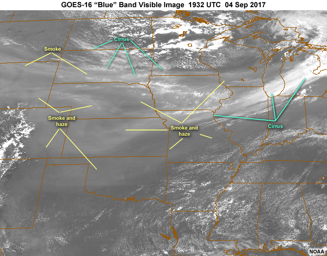
Atmospheric aerosols scatter incoming visible radiation that varies depending on the size of the airborne particle and wavelength. Smaller particles tend to scatter more light at shorter wavelengths as we see in this comparison of the “blue”, “red”, and "veggie" band images on a day when smoke from western fires advected into the region. In the "veggie" band image, we see that smoke and haze over land are mostly undetectable, with the dominant signal coming from surface features and clouds.

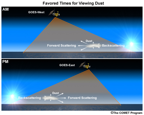
The GOES-R 0.47 micrometer band is particularly well suited for detecting haze, smoke, dust and pollution, especially early or late in the day as sun angles become lower and more energy is forward scattered toward the satellite detectors. As the figure shows, GOES-West is most sensitive to scattering by aerosols over North America during the early morning hours, whereas viewing of aerosols by GOES-East becomes more favorable later in the day.

These visible and "veggie" band animations are for the same day shown earlier. Notice that more haze, smoke and pollution are evident later in the day as the sun-satellite geometry becomes more favorable for viewing atmospheric aerosols.

Click the tabs to compare and contrast the appearance of haze and smoke in the "blue", "red", and "veggie" bands.

Scattering » Smoke

Smoke from wildland fires and agricultural burning scatters visible sunlight in much the same way as other aerosols. With smoke scattering more sunlight at shorter visible wavelengths, the ABI’s “blue” band will generally detect more smoke than the “red” and "veggie" bands, especially over land. Notice in the animations that smoke becomes more noticeable later in the day as more energy is forward scattered toward the Himawari-8 satellite which is located to the east of the Asian continent. We also see that the “red” and "veggie" bands are somewhat better at detecting smoke over open water because of water’s relatively poor reflectance.

Scattering » Blowing Dust

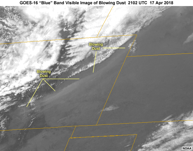
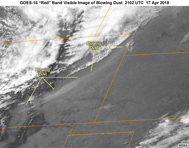
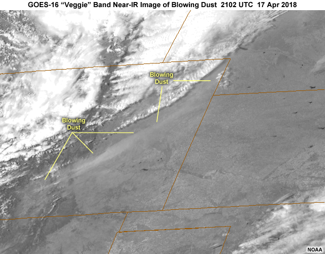
The images show an extensive dust plume over eastern Colorado being generated by strong southwesterly winds out ahead of a vigorous springtime storm system.

While contrast between blowing dust and nearby land surfaces is poorer in the “blue” band, thinner layers of dust are more detectable since dust and other aerosols scatter more sunlight at shorter visible wavelengths. In many instances, thin layers of dust may not even be detectable in the “red” band.

For thick opaque dust layers however, "dust" particles are more reflective in the "red" band than at shorter visible wavelengths as shown on the right side of this illustration. This enhances the contrast between dust and Earth's surface, especially over green vegetation and water which are poorly reflective in the "red" band. RGB imagery and other derived products can take advantage of dust's "blue" vs. "red" band reflective difference to improve daytime dust detection, especially when combined with infrared techniques that take advantage of the thermal contrast between elevated dust and the surface.

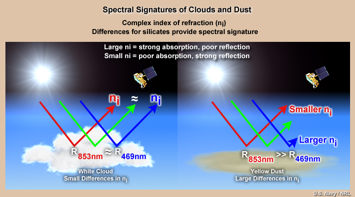
In the "veggie" band, blowing dust is readily apparent over darker water surfaces, but is more difficult to see over land due to its brighter more reflective properties.

As with other aerosols, for this example's sun-satellite viewing geometry, dust becomes brighter in all three bands later in the day as more sunlight is forward scattered toward the satellite.

Drag the slider to compare the three GOES-16 "blue", "red", and "veggie" bands.

Enhancements

GOES-R+ ABI visible imagery with its 12-bit grayscale depth provides information over a useful dynamic range that extends far beyond the eye's ability to discriminate variations of gray. Enhancement may be required to make full use of the information available from GOES-R. Different enhancements, for low light situations versus bright cloud-filled scenes at midday, allow details to be detected that would go unnoticed using one standard enhancement.

To explore different enhancements and their application to various meteorological scenarios, see the COMET lesson, GOES Channel Selection V2.

Summary

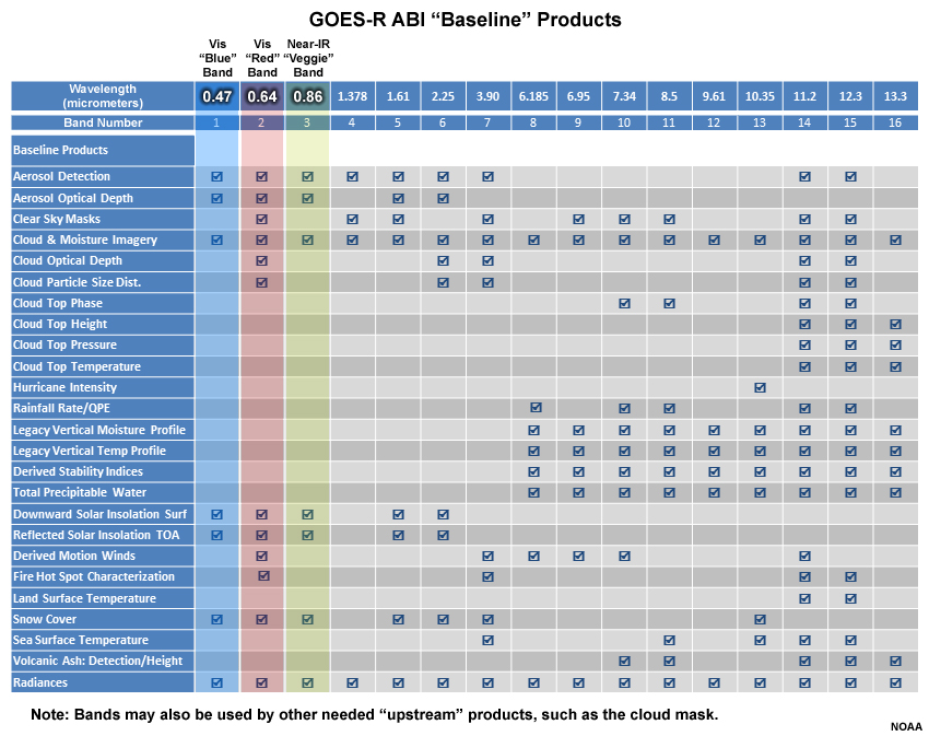
The ABI's two visible bands and 0.86 µm near-IR band will provide forecasters with high spatial and temporal resolution imagery and products for monitoring a variety of surface and atmospheric phenomena, some of which were highlighted in this lesson. In addition to imagery, these three bands will contribute to a host of "baseline" derived products shown in this table. Based on scientific algorithms, these products provide quantitative data on various physical properties by extracting information from different band groupings known to be sensitive to that property.

Visible and Near-IR Band Characteristics:

• Spectral Coverage
  • “blue” band: 0.47 µm central wavelength, 0.451 – 0.491 μm (GOES-R ABI), Visible
  • “red” band: 0.64 µm central wavelength, 0.596 – 0.682 μm (GOES-R ABI), Visible
  • "veggie" band: 0.86 µm central wavelength, 0.847 – 0.882 μm (GOES-R ABI), Near-Infrared
• Resolution
  • “blue” band: 1-km field of view
  • “red” band: 0.5-km field of view
  • "veggie" band: 1-km field of view
• Quality Improvements
  • Low noise and improved pixel geolocation and registration (frame to frame pixel stability)

Application Considerations:

• Available daytime only
• Bands see scattered and reflected energy
• See clouds and Earth's surface
• Sensitive to soil, water, and cloud type; “red” and "veggie" bands more sensitive to surface variation
• “Red” band sensitive to suspended sediment and turbid waters
• Sense haze, smoke, and dust particularly early and late in the day depending on sun-satellite geometry (more forward scattering); “blue” band more sensitive to scattering by aerosols than “red” and "veggie" bands
• Optimal use may require enhancement
• Shadows can be used for estimating cloud heights

You have reached the end of the lesson. Please complete the quiz and share your feedback with us via the user survey.

Resources

Internet Resources

• Official GOES-R Program Site, http://www.goes-r.gov/
• GOES-R Training Overview, http://www.goes-r.gov/users/training.html
• GOES-R: Benefits of Next-Generation Environmental Monitoring, http://www.meted.ucar.edu/training_module.php?id=509
• GOES-R Proving Ground Page, http://www.goes-r.gov/users/proving-ground.html
• GOES-R Documentation Page, http://www.goes-r.gov/resources/docs.html
• GOES-R Scientific Publications, http://www.goes-r.gov/resources/Scipubs/index.html
• GOES and POES Conferences and Meetings, http://www.goes-r.gov/users/conf-mtgs.html
• UW CIMSS Satellite blog and GOES-R, http://cimss.ssec.wisc.edu/goes/blog/archives/category/goes-r
• VISIT: SHyMet for Forecasters: GOES-R 101 Training Session, http://rammb.cira.colostate.edu/training/shymet/forecaster_goesr101.asp

Advanced Baseline Imager (ABI) Specific

• GOES-R ABI Instrument Page, http://www.goes-r.gov/spacesegment/abi.html
• GOES-R ABI: Next Generation Satellite Imaging, http://www.meted.ucar.edu/training_module.php?id=987
• ABI Fact Sheet, http://www.goes-r.gov/education/docs/Factsheet_ABI.pdf
• ABI Bands Quick Information Guides, http://www.goes-r.gov/education/ABI-bands-quick-info.html

 

References

GOES-R

• Schmit, T., P. Griffith, M. Gunshor, J. Daniels, S. Goodman, and W. Lebair, 2017: A closer look at the ABI on the GOES-R series. Bull. Amer. Meteor. Soc., 98, 681-698, doi: https://doi.org/10.1175/BAMS-D-15-00230.1.
• Schmit, T.J., S.S. Lindstrom, J.J. Gerth, and M.M. Gunshor, 2018: Applications of the 16 spectral bands on the Advanced Baseline Imager (ABI). J. Operational Meteor., 6, 33-46, doi: https://doi.org/10.15191/nwajom.2018.0604.
• Additional GOES-R and GOES Related Scientific Publications and other documentation (available on the GOES-R Program Site):
  Publications: http://www.goes-r.gov/resources/Scipubs/index.html
  Documentation: http://www.goes-r.gov/resources/docs.html

Contributors

COMET Sponsors

MetEd and the COMET® Program are a part of the University Corporation for Atmospheric Research's (UCAR's) Community Programs (UCP) and are sponsored by

• NOAA's National Weather Service (NWS)
  with additional funding by:
• Bureau of Meteorology of Australia (BoM)
• Bureau of Reclamation, United States Department of the Interior
• European Organisation for the Exploitation of Meteorological Satellites (EUMETSAT)
• Meteorological Service of Canada (MSC)
• NOAA's National Environmental Satellite, Data and Information Service (NESDIS)
• NOAA's National Geodetic Survey (NGS)
• National Science Foundation (NSF)
• Naval Meteorology and Oceanography Command (NMOC)
• U.S. Army Corps of Engineers (USACE)

To learn more about us, please visit the COMET website.

Project Contributors

Program Managers

• Wendy Abshire – UCAR/COMET
• Bruce Muller – UCAR/COMET

Project Lead and Meteorologist

• Patrick Dills — UCAR/COMET

Instructional Design

• Bruce Muller — UCAR/COMET

Science Advisors and Contributors

• Dr. Jordan Gerth — Cooperative Institute for Meteorological Satellite Studies (CIMSS)/NOAA/University of Wisconsin
• Tim Schmit — NOAA NESDIS STAR/ASPB @ CIMSS

Graphics/Animations

• Steve Deyo — UCAR/COMET

Multimedia Authoring/Interface Design

• Gary Pacheco — UCAR/COMET

Audio/Video Editing/Production

• Steve Deyo – UCAR/COMET

Audio Narration

• Vanessa Vincente — UCAR/COMET

GOES-16 Imagery Provided By

• NOAA

Himawari-8 Imagery Provided By

• SSEC/Unidata Community ADDE Open Archive – University of Wisconsin, Madison
• Japan Meteorological Agency (JMA)

COMET Staff, August 2018

Director's Office

• Dr. Elizabeth Mulvihill Page, Director
• Tim Alberta, Assistant Director Operations and IT
• Paul Kucera, Assistant Director International Programs

Business Administration

• Lorrie Alberta, Administrator
• Auliya McCauley-Hartner, Administrative Assistant
• Tara Torres, Program Coordinator

IT Services

• Bob Bubon, Systems Administrator
• Joshua Hepp, Student Assistant
• Joey Rener, Software Engineer
• Malte Winkler, Software Engineer

Instructional Services

• Dr. Alan Bol, Scientist/Instructional Designer
• Tsvetomir Ross-Lazarov, Instructional Designer

International Programs

• Rosario Alfaro Ocampo, Translator/Meteorologist
• David Russi, Translations Coordinator
• Martin Steinson, Project Manager

Production and Media Services

• Steve Deyo, Graphic and 3D Designer
• Dolores Kiessling, Software Engineer
• Gary Pacheco, Web Designer and Developer
• Sylvia Quesada, Production Assistant

Science Group

• Dr. William Bua, Meteorologist
• Patrick Dills, Meteorologist
• Bryan Guarente, Instructional Designer/Meteorologist
• Matthew Kelsch, Hydrometeorologist
• Erin Regan, Student Assistant
• Andrea Smith, Meteorologist
• Amy Stevermer, Meteorologist
• Vanessa Vincente, Meteorologist