About the Lesson
This lesson introduces you to seven of the ten infrared imager bands on the GOES R-U ABI (Advanced Baseline Imager). By exploring the spectral characteristics of each band, you will gain a better understanding of band selection and what each band observes, and begin to appreciate some of the many potential applications.
Please note that information on the three water vapor bands not included here can be found in the IR Water Vapor Bands lesson.
On completing the lesson, you should be able to:
- Identify the various phenomena that can be detected in the seven ABI infrared bands covered in this lesson
- Identify sun glint in shortwave infrared imagery
- Identify which band is sensitive to hot spots and daytime aerosols
- Describe what is meant by "clean" vs. "dirty" infrared window bands
- Identify which band is most sensitive to stratospheric ozone
- Identify which bands are sensitive to emissions of volcanic sulfur dioxide
- Identify the bands useful for determining cloud properties
Please note that this lesson was originally published prior to the launch of GOES-16 and used imagery from the Himawari-8 geostationary satellite to illustrate GOES-R ABI capabilities. The Himawari-8 imager, the AHI (or Advanced Himawari Imager), has bands nearly identical to the ABI on board the GOES R to U series. In the interest of time, some of the original Himawari-8 imagery is still included where geographical context is not critical for understanding the concept.
Introduction
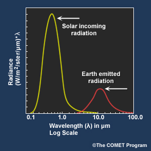
The earth and atmosphere emit energy primarily in the infrared at wavelengths greater than about 3 micrometers and peaking near 10 micrometers. The Advanced Baseline Imager's (ABI) infrared bands are in the 3 to 14 micrometer region of the infrared spectrum where much of this peak emission occurs.
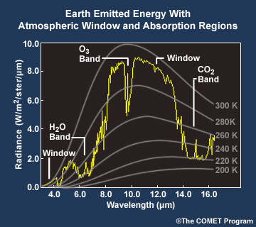
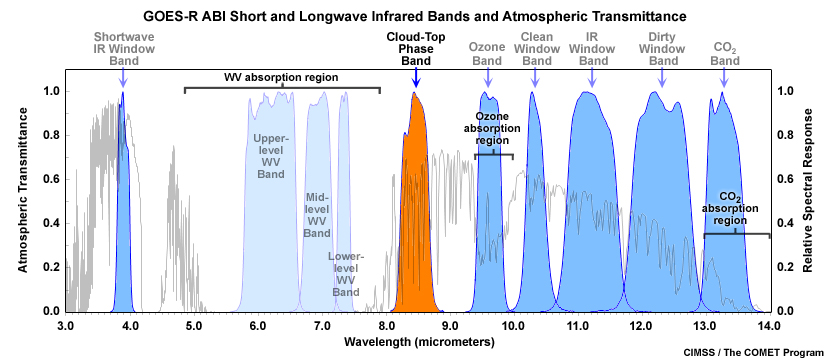
Atmospheric gases absorb selectively in the longwave infrared, particularly water vapor between 5 and 8 micrometers, ozone between 9.2 and 9.8 micrometers, and carbon dioxide at wavelengths greater than 13 micrometers. Outside these major gas absorption regions, the clear atmosphere is highly transparent to longwave infrared radiation. Window regions are denoted "clean" when very little atmospheric absorption is present, and "dirty" when there is some absorption by gases, but not enough to prevent energy from the surface and clouds from reaching the satellite.
The amount of energy emitted depends on the temperature and emissivity (emission efficiency) of the earth's surface, clouds, aerosols and gases.
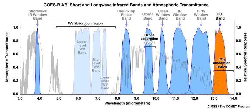
Atmospheric gases absorb and re-emit infrared energy at discrete wavelengths. The jagged yellow earth emitted radiance curve shown in the graphic, varies with wavelength due to absorption and emission by gases at different pressure levels. We'll explore this further as we step through the individual bands.
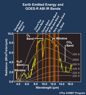
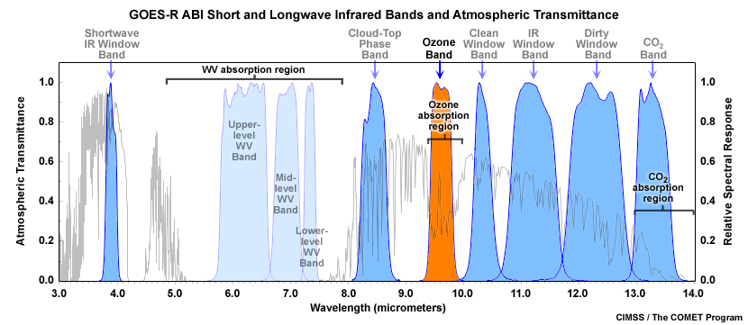
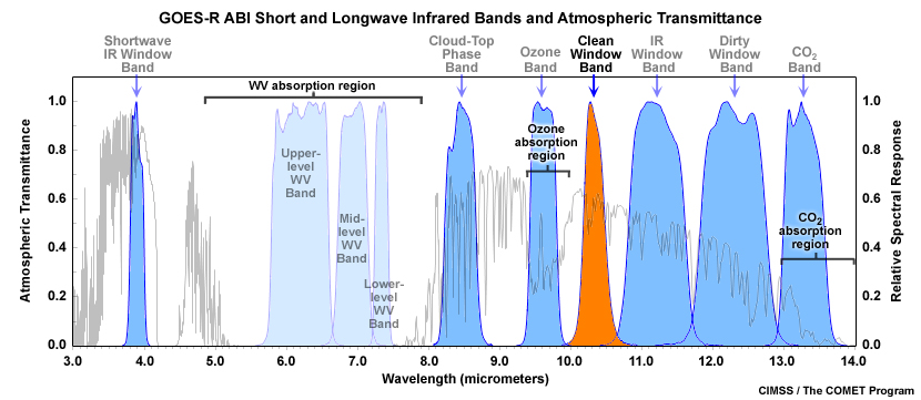
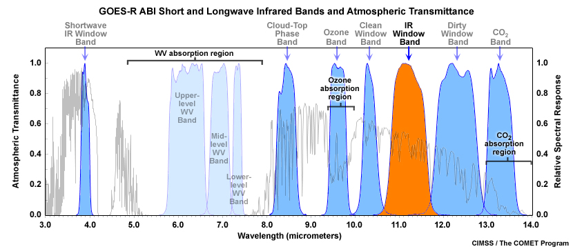
When superimposing the various infrared band locations, we see that some are located in infrared "window" regions where we see Earth's surface and clouds without a significant contribution from atmospheric gases. Other bands are sensitive to absorption by gases, with the degree of sensitivity determining the relative mix of atmosphere, clouds, and surface we'll be able to see. As a general rule, the greater the band's sensitivity to a gas, the higher the altitude the infrared signal originates from, and the less emission we'll see from the surface and lower atmospheric layers, including cloud cover.
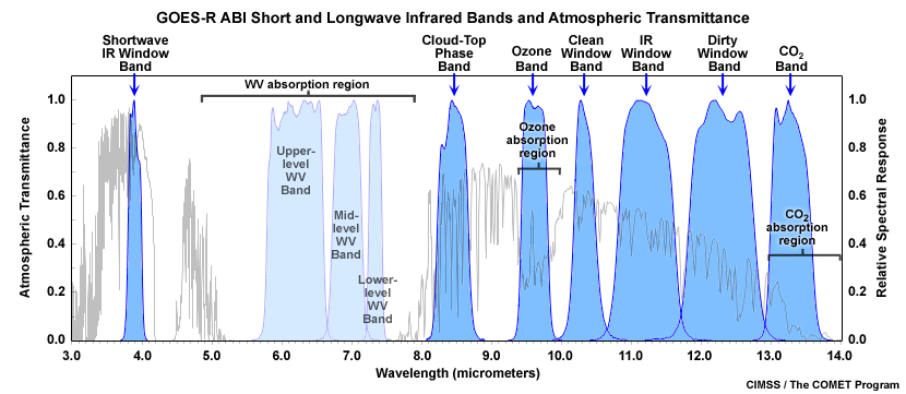
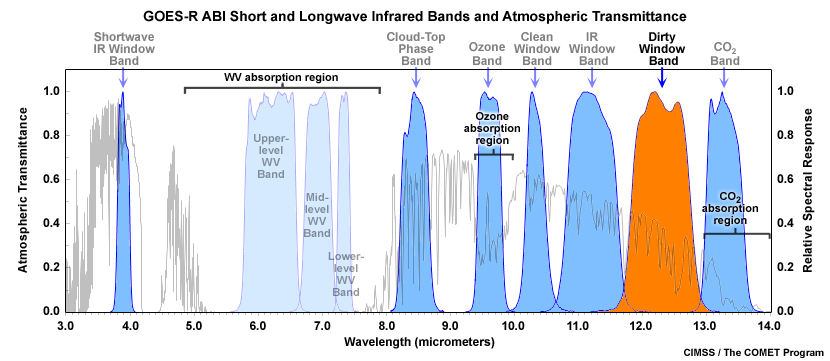
Another convenient way to show the impact of selective absorption on the ABI's infrared bands is to plot total atmospheric transmittance as a function of wavelength. In the graph below, the gray jagged background curve is atmospheric transmittance shown for a representative atmosphere. When transmittance approaches one (or 100%), most Earth-emitted energy reaches space. And when transmittance dips to smaller values, that implies more absorption by gases and therefore less energy reaching space. Zero transmittance would be an atmosphere that's totally opaque and very cold from a satellite's vantage point. The blue shaded curves represent the instrument response functions for ABI's IR window bands and show the spectral interval covered by each band.
Now let's look at each of the seven infrared bands covered in this lesson beginning with the 3.9 "shortwave IR window" band.
Shortwave IR Window Band
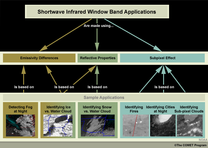
The shortwave IR window band at 3.9 micrometers has demonstrated its usefulness for many applications on board both geostationary and polar-orbiting meteorological satellites since the late 1970s. Some of these applications include:
- An improved ability to identify and monitor the evolution of fog and low clouds
- Cloud phase determination
- Delineating between supercooled water and ice clouds
- Locating water clouds over snow during daytime
- Detecting hot spots such as fires and volcanoes
- Monitoring atmospheric aerosols and volcanic ash during daytime
- Sea-surface temperature measurements at night, and
- Estimating low-level cloud motion winds
The chart shown here summarizes three radiative transfer concepts that are key for exploiting the many capabilities of the shortwave IR band. We'll touch briefly on each concept in this section.
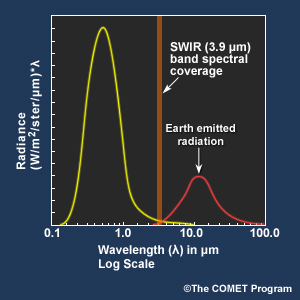
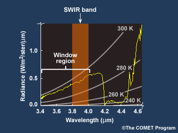
The shortwave IR band is located in the shortwave window region of Earth's emitted spectrum. Radiation in this region is not significantly absorbed by Earth's atmosphere. There is also much less earth-emitted energy in this wavelength region than at longer wavelengths.
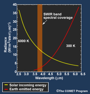
The spectral region covered by the shortwave IR band also includes reflected solar radiation. In the zoomed in plot, we see that there is an overlap in the region covered by the shortwave IR band. The addition of reflected solar radiation from clouds and land produces a noticeable warming effect when viewing daytime shortwave IR imagery.
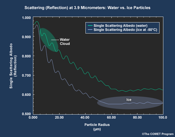
Large differences in the scattering (reflection) properties of water and ice particles in the shortwave infrared allow the shortwave IR band to discriminate cloud phase and detect snow cover during daytime.
The graph below shows that reflection at 3.9 micrometers by a cloud, is a function of both cloud phase and droplet size. Droplet radii in water clouds range between 5 and 20 micrometers, while ice particles in cirrus clouds are often 50 micrometers or larger. Therefore, water clouds are much more reflective (warmer) than ice clouds at 3.9 micrometers during daytime.
During nighttime, the emissivity (or emission efficiency) of water clouds at 3.9 micrometers is less than at longer infrared wavelengths. This results in colder brightness temperatures for water clouds in the shortwave IR band than in the longwave IR bands. For relatively thin cirrus however, the reverse is true.
Notice in the image comparison that thin cirrus appear warmer while lower level liquid water cloud tops appear cooler.
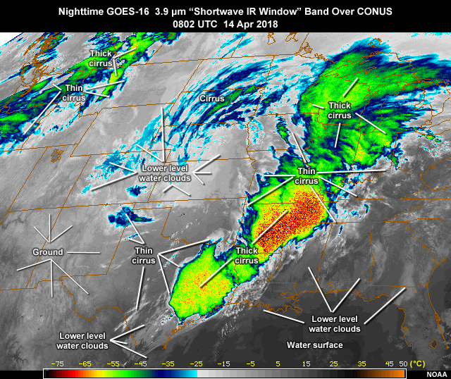
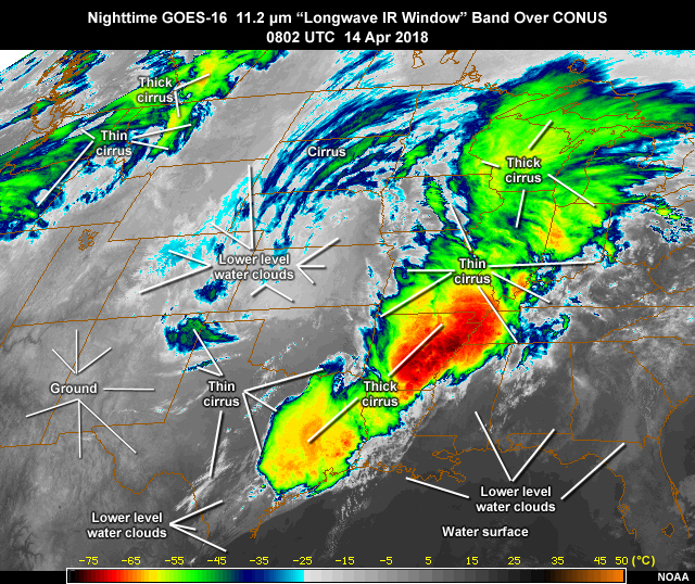
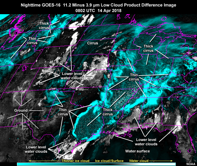
The shortwave and longwave IR bands have long been used in combination, typically by employing a difference technique to produce a nighttime image product that delineates ice and water clouds.
Detection of fires and hot spots is another special capability of the shortwave IR band. A band near 3.9 micrometers is much more sensitive in terms of the energy detected by the satellite when the temperature of an object increases, than a band centered near 11 micrometers. This effect is noticeable when an image pixel is partially filled by a hot spot or fire.
A plot for brightness temperatures for subpixel fires is shown in the left panel. The 3.9 micrometer brightness temperature is measurably warmer than the 10.7 micrometer temperature, especially for small values of N (hot spot fractional coverage).
A similar warming effect can be seen for subpixel cloud cover where cloud top temperatures are typically colder than the surrounding surface. Comparing the 3.9 micrometer band with either the 10.3 or 11.2 micrometer bands for a scene with small cumulus cloud elements for example, we would expect the 3.9 micrometer image to appear slightly warmer.
The animation below shows a very active brushfire as it appears in color enhanced 3.9 micrometer band imagery beginning in the overnight hours. Thicker portions of the smoke plume are also evident given the band's sensitivity to larger aerosol particles.
As the loop enters daytime, solar energy reflects off the surrounding land surfaces and hence we see warmer brightness temperatures. Some of the warming (in brightness temperatures) is also due to infrared emission from a warming surface. Despite the additional solar input, the fire's hotspots remain visible. Some of this is due to the band's increased saturation temperature on AHI and ABI. The newer 3.9 micrometer band saturates at 410 K, which is about 70 K warmer than with legacy GOES. This allows for improved identification of fires, distinguishing a fire from nearby hot reflective surfaces for example, and for better sub-pixel fire characterization such as a fire's aerial coverage and burn temperature.
As in the visible and near-IR, sun glint must be considered when viewing shortwave IR imagery over water areas. When water surfaces are smooth, large reflections occur when the sun and satellite are properly aligned.
Two different image enhancements are shown in the loops below. The loop on the left uses brighter shades to indicate warmer brightness temperatures and darker shades to indicate colder brightness temperatures. The loop on the right uses a proposed AWIPS IR color enhancement.
Notice the bright relatively warm region moves from east to west as the sun moves. We also see patches that are relatively warm and cold within the larger glint pattern. Some patches change from colder to warmer as the sun's reflection approaches, and then back again. These are indicative of relatively calm waters surrounded by a rougher sea surface.
Cloud-top Phase Band
Located at the edge of the longwave IR window region, the ABI's 8.4 micrometer "cloud-top phase" band is new to the GOES satellites.
While similar to longwave IR window bands in the 10 to 12 micrometer region, the 8.4 micrometer band has an additional capability to help determine cloud-top microphysical properties during both day and nighttime. The sample cloud type product image shown below combines information from the AHI's 8.4, 11.2, and 12.4 micrometer bands and will also be available from GOES-R.
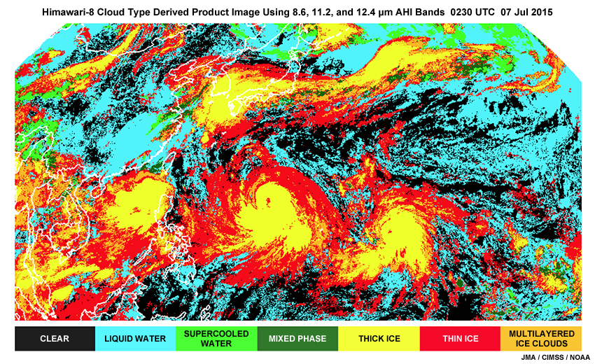
Combining the 8.4 and 11.2 micrometer bands allows for a more consistent day-night discrimination between water and ice clouds when compared to the more "traditional" fog/low cloud product which is limited to nighttime use due to daytime solar contamination.
Similar to the 3.9 micrometer band at night, the emissivity of dense water cloud tops at 8.4 micrometers is less than at 11.2 micrometers, resulting in cooler cloud tops at 8.4 than at 11.2 micrometers. In contrast, ice clouds tend to have much smaller temperature differences and even of the opposite sign for thinner cirrus.
Drag the slider to compare water vs. ice cloud-top brightness temperatures for the 8.4 and 11.2 micrometer images.
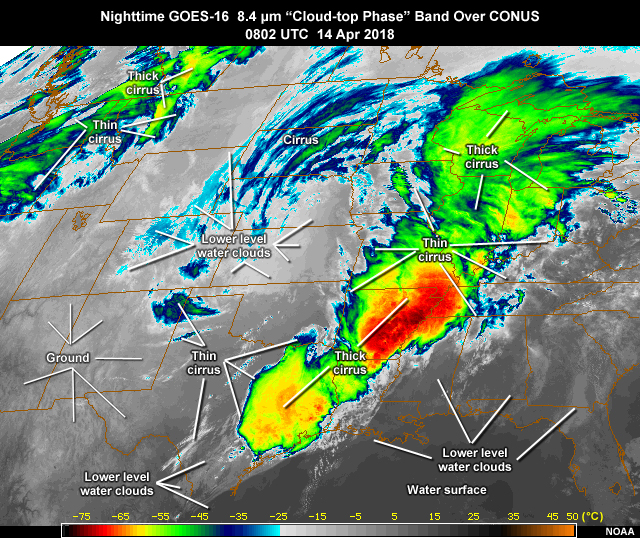
Notice near the center of the images (Wyoming, Colorado, Nebraska, Kansas) that lower level water clouds appear colder at 8.4 than at 11.2 µm. Thinner cirrus on the other hand appears warmer at 8.4 than at 11.2 µm. (seen in the upper portion of the images and around the edges of thick convective cirrus in the lower and right portion of the images). Ground (in the lower left) and water surfaces (bottom center and right) typically have nearly the same brightness temperature in both bands, but may appear slightly cooler in the 8.4 µm band due to its greater sensitiviy to low level moisture compared to the 11.2 µm band.
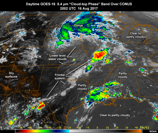
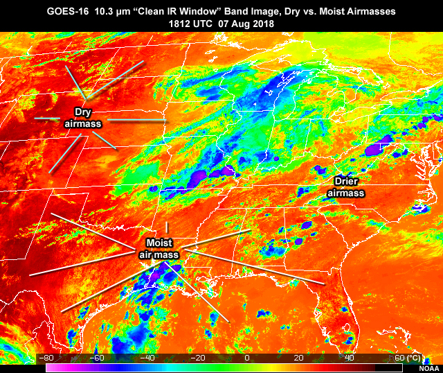
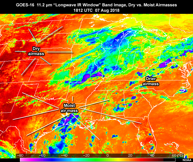
The ABI's 8.4 micrometer band also is lies in a "dirty" window region where water vapor absorption is stronger than in the 10.3 and 11.2 micrometer window bands. This results in brightness temperatures for surface features that are slightly cooler in the presence of a moist low-level atmosphere.
For desert scenes, despite a typically dryer lower atmosphere, cooler 8.4 micrometer brightness temperatures relative to the 10.3 and 11.2 bands, are common as well. This is the result of a surface emissivity (or emission effiency) for a desert surface that's typically around 90%, compared to darker soil types and vegetation cover where emissivities are closer to 100%.
The scene below shows the cooling effect in the 8.4 micrometer band compared to the 10.3 clean IR window band. Drier areas of the Intermountain West are compared to the more temperate and moist regions of the eastern U.S.
The 8.4 micrometer band, when combined with the 11.2 and 12.3 micrometer bands, is also useful for detecting volcanic ash clouds containing aerosols and sulfur dioxide (SO2), especially for large concentrations of SO2.
The atmospheric transmission plot for SO2 shows two distinct absorption bands in the infrared. Notice that SO2 absorption in the 8.4 micrometer band becomes pronounced only as SO2 concentrations become quite large.
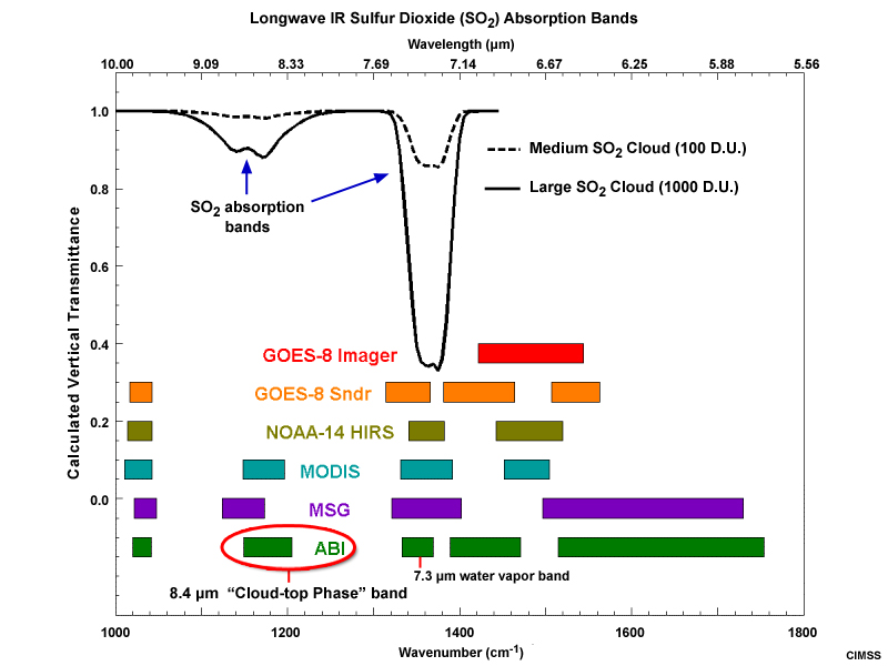
Since SO2 concentrations tend to be greatest in the lower troposphere, any SO2 signal, seen as cooling in the 8.4 µm band, is more indicative of an SO2 event in the lower troposphere. For detecting smaller concentrations of SO2, which is more likely in the upper troposphere, the 7.3 µm water vapor band is more effective given its greater sensitivity to SO2.
Ozone Band
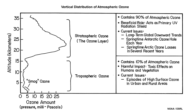
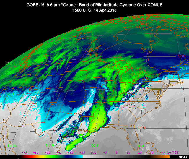
The ABI's 9.6 micrometer "ozone" band is located in a strong ozone absorption region within Earth's infrared emitted spectrum.
Despite spatial variations, 90% of Earth's ozone resides in the stratosphere and with large concentrations just above the tropopause. This means that most of the ozone signal in this band originates from layers near and above the tropopause.
The ozone band is also slightly sensitive to water vapor, such that the combined absorption effects of ozone and water vapor will result in imagery that generally appears cooler than in the IR window bands. Cloud tops near or extending above the tropopause may however appear warmer in the ozone band due to ozone emissions from the lower stratosphere where temperature increases with height.
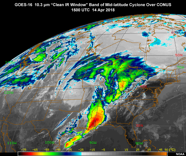
Drag the slider to compare a 9.6 micrometer ozone band image with the corresponding 10.3 micrometer clean IR window band.
The ozone band's brightness temperatures are also sensitive to changes in satellite viewing (or zenith) angle. As the satellite scans farther away from nadir, the point directly beneath the satellite above the equator, the scan angle increases and energy is detected from higher in the atmosphere.
In the weighting function animation below, notice that the stratospheric ozone contribution increases as the viewing angle approaches the limb near 70 degrees, and the brightness temperature 'T sub b' decreases. We can also see the ozone band's water vapor absorption as a contribution in the lower troposphere. Assuming a moist atmosphere, the height of that contribution also increases slightly with increasing scan angle, resulting in an additional cooling effect.
Looking at the ozone band image for a moment, we see that brightness temperatures cool with increasing distance away from the satellite's subpoint above the equator. The effect is more pronounced toward the poles since stratospheric ozone concentrations are greater there than along the equator. This cooling phenomenon, known as "limb darkening", is particularly pronounced for scan angles greater than 60 degrees. Limb darkening affects all of the IR bands since they all experience at least some degree of absorption by gases, but is most noticeable in the ozone and carbon dioxide bands where absorption is strongest.
Clean Longwave IR Window Band
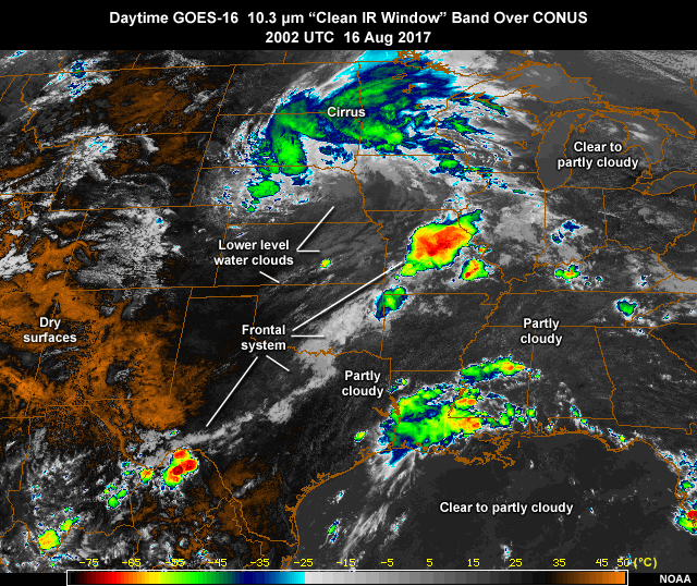
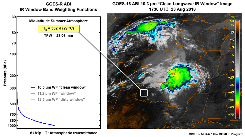
The ABI's 10.3 micrometer "clean longwave IR window" band is one of four ABI infrared window bands. It's located in a window region of the IR spectrum with little sensitivity to absorption by water vapor, and is also the least sensitive to water vapor of the four longwave IR window bands (at 8.4, 10.3, 11.2, and 12.3 micrometers). This suggests that the 10.3 micrometer band provides the "cleanest" view of both cloud tops and Earth's surface.
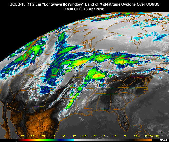
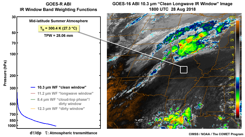
The weighting functions (or contribution functions) shown below are for the four IR window bands under clear-sky conditions, with the 10.3 micrometer band's curve highlighted in blue. The area under and to the left of each curve indicates the relative contributions to the outgoing energy from various layers of the atmosphere. We see that all four weighting functions peak at the surface. This reinforces the point that the satellite brightness temperature signal is dominated by the surface for cloud-free scenes in all four IR window bands.
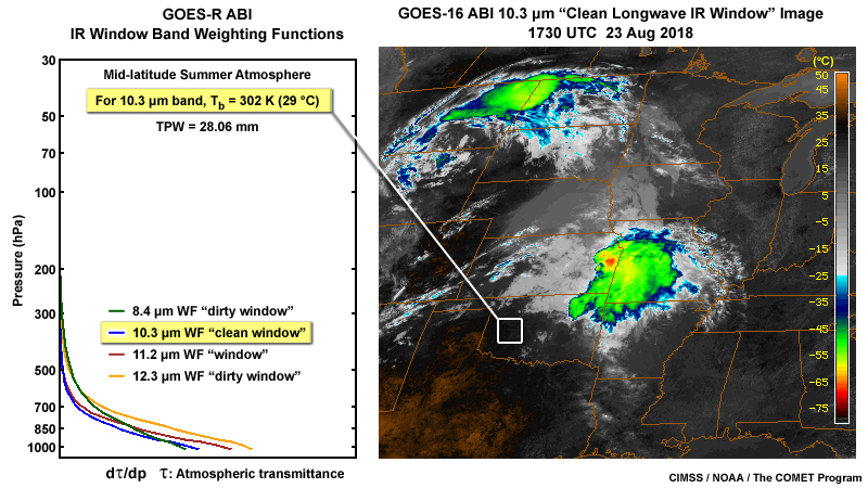
The figure's left panel depicts weighting functions for clear sky scenes for the ABI's four IR window bands (at 8.4, 10.3, 11.2, and 12.3 µm). The right panel is a 10.3 µm clean window band image showing a late summer mid-latitude cyclone over the Northern Rockies and Central U.S.
At the 10.3 micrometer wavelength, most surfaces and cloud types have an emissivity close to 1 (that's 100% in terms of efficiency), with a notable exception being thin cirrus. Therefore, the brightness temperature sensed by the satellite is close to actual surface skin or cloud-top temperature for scenes other than thin cirrus. Actually, thin cirrus permits more energy to pass through it than in the other IR window bands, and will therefore appear warmer in the 10.3 micrometer band.
For most surface features, the 10.3 micrometer band is also slightly warmer than traditional IR window bands due to its relatively weak sensitivity to lower tropospheric moisture.
The comparison below highlights some of the more commonly seen differences between the 10.3 and more traditional 11.2 micrometer bands. Given the similarity between these two IR bands, the 10.3 micrometer clean window band can be used much like the 10.7 micrometer band on legacy GOES as well as the Suomi-NPP and JPSS polar-orbiting satellites.
Drag the slider to compare 10.3 and 11.2 micrometer band images over the Southeastern U.S. during early summer.
Please note: The two images have been enhanced with the Rainbow IR color table to better highlight subtle temperature differences between the two spectral bands.
For derived products, the 10.3 micrometer band's "clean window" quality helps with improving atmospheric moisture corrections in SST and other surface products, estimating moisture profiles, estimating cloud-top particle size, and characterizing surface properties.
Longwave IR Window Band
Familiar to most as the traditional longwave infrared band or channel, the ABI's 11.2 micrometer "longwave IR window" band is the third of four ABI IR window bands covered in this lesson. It's located in a window region of the IR spectrum with only minor sensitivity to absorption by water vapor. As with the other three window bands, the result is a brightness temperature signal dominated by the temperature signal from cloud tops and the surface.
At the 11.2 micrometer wavelength, similar to the 10.3 micrometer band, most surfaces and cloud types have an emissivity close to 1 (that's 100% in terms of efficiency). Therefore, the brightness temperature sensed by the satellite is close to actual surface skin or cloud-top temperature for scenes other than thin cirrus.
Less longwave IR energy escapes to space through optically thin (semi-transparent) cirrus in the 11.2 micrometer band compared to the 10.3 micrometer band. Therefore, cirrus that is not opaque will appear cooler in the 11.2 micrometer band. The 12.3 micrometer dirty window band allows even less longwave energy to transit a thin cloud, so cirrus clouds will appear even cooler in that band.
In the images below, we see that thinner cirrus appears progressively cooler as the wavelength increases from 10.3 to 11.2 and then to 12.3 micrometers. Surface features appear progressively cooler as well, something we'll explore more in a moment.
Drag the slider to compare the GOES-16 IR images showing hurricane Harvey.

Drag the slider (above) to compare the GOES-16 IR images.
The weighting functions (or contribution functions) shown below include the ABI's four IR window bands under clear-sky conditions, with the 11.2 micrometer curve colored brown. The area under and to the left of each curve indicates the relative contributions to the outgoing energy from various layers of the atmosphere.
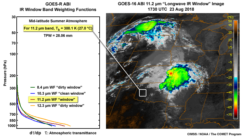
While all four weighting functions peak at the surface, we see that the 11.2 micrometer curve is located to the right of the 10.3 micrometer band curve below about 700 millibars. This indicates a greater sensitivity to lower tropospheric water vapor than at 10.3 micrometers. The result is a brightness temperature for clear-sky scenes that is slightly cooler in the 11.2 vs. the 10.3 micrometer band, but still warmer compared to the 8.4 and 12.3 micrometer bands where water vapor sensitivity is stronger. The cooling effect in the 8.4, 11.2, and 12.3 micrometer bands increases as low-level moisture increases, which has implications for assessing low-level moisture and diagnosing air mass boundaries.
Drag the slider to compare the 8.4, 10.3, 11.2 and 12.3 micrometer weighting functions and images.
Drag the slider (above) to compare the four IR window band weighting functions and GOES-16 images.
GOES-R improvements for the IR bands include a 2-km spatial resolution, 15-minute refresh rate over the full Earth disc, 5-minute refresh rate over the extended contiguous U.S., and an even more frequent 1-minute cadence for two movable areas. With these improvements, the 11.2 micrometer band gives meteorologists an unprecedented ability to monitor the evolution, upscale growth, and decay of convection via cloud-top temperatures in conjunction with radar and the GOES-R GLM's ground breaking lightning observations.
The GOES-R ABI images routinely across the contiguous U.S. every 5 minutes and at least every 15 minutes across the full Earth disk.
The 11.2 micrometer band is also a significant contributor to all three main GOES-R derived product areas including: baseline, future capability, and envisioned. Examples for baseline products include imagery, cloud properties, satellite derived winds, sea surface temperature, and total precipitable water. Examples of future capability products include overshooting tops and total ozone. And the final class of products are those envisioned as follow-on applications that go beyond conventional uses of satellite information to include decision aids for improved predictions of convection and severe weather.
Dirty Longwave IR Window Band
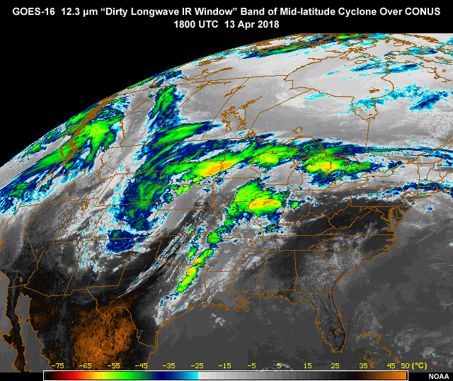
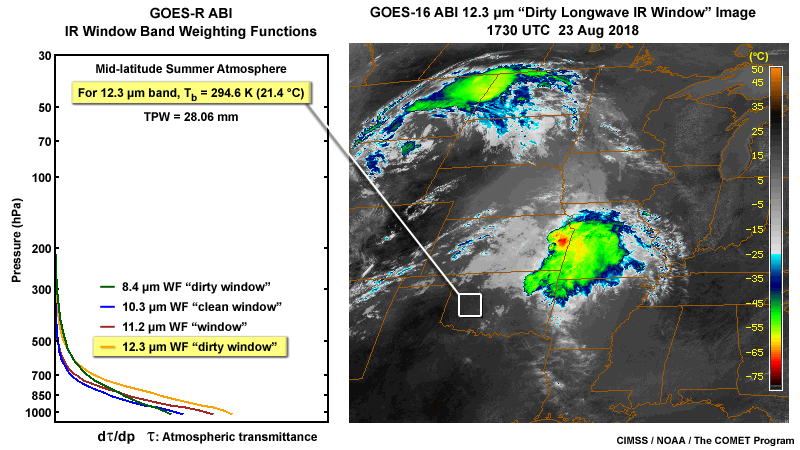
As with the other three longwave IR window bands, the ABI's 12.3 micrometer band is located in the broad longwave IR window region. Of this IR band grouping, the 12.3 micrometer band is the most sensitive to absorption by low-level atmospheric moisture, hence its naming as the "dirty" longwave IR window band.
Similar bands have been available on both GEO and LEO satellites for many years due to this band's many uses. In combination with a cleaner IR window band, the 12.3 micrometer band can be used to estimate low-level moisture, analyze air mass differences and boundaries, diagnose cloud properties, and both observe and quantify volcanic ash, airborne dust and sand.
As with the 10.3 and 11.2 micrometer bands, most surfaces and thick opaque clouds have an emissivity in the 12.3 micrometer band close to 1. Beyond emissivity however, there are subtle yet important differences related to the band's sensitivity to low-level moisture, and more complex absorption and scattering processes within water and ice clouds, dust, and volcanic ash. These optical properties make the 12.3 micrometer band particularly useful in combination with other IR bands for numerous applications as we'll explore a bit further.
One such combination of different IR bands is what's known as a "split window difference" that uses the 12.3 micrometer band and a cleaner IR window band such as the 11.2 micrometer band. The difference product is particularly good for highlighting a variety of atmospheric and cloud properties already mentioned.
Let's look at identification of thin cirrus for a moment, a long standing use of the 12.3 micrometer band. Ice cloud particles absorb more energy at 12.3 micrometers than in the 8.4, 10.3 and 11.2 micrometer bands. This reduces the brightness temperature of thinner cirrus compared to the other three IR window bands. In the image comparison below, we see that thinner cirrus appear progressively cooler as wavelength increases from 10.3 to 12.3 micrometer wavelengths. Surface features also appear progressively cooler, something we'll look at next.
Drag the slider to compare the GOES-16 IR images showing hurricane Harvey.
Drag the slider (above) to compare the GOES-16 IR images.
As mentioned earlier, the 12.3 micrometer band is the most sensitive to atmospheric moisture of the four IR window bands. Weighting functions (or contribution functions) for the ABI's four IR window bands are shown below for clear-sky conditions and for a relatively moist summertime mid-latitude atmosphere. The 12.3 micrometer band's curve is colored orange.
Focusing on the 12.3 micrometer weighting function, we see that the curve is located farthest to the right of the four IR window bands with much of contribution due to water vapor absorption occurring below about 700 millibars. This indicates a more significant sensitivity to lower tropospheric water vapor. The result is a brightness temperature for clear-sky scenes that is slightly cooler compared to the other three bands, assuming that no strong temperature inversions are present within this layer.
In the three weighting functions below, notice that for most scenes, brightness temperatures cool with increasing wavelength, where there is greater sensitivity to low-level moisture.
Drag the slider (above) to compare the three IR window band weighting functions and images.
The cooling effect also increases as the amount of low-level moisture increases, being most notable in the 12.3 micrometer band. More moisture usually causes more cooling as water vapor absorption occurs higher in the troposphere. This has implications for estimating low-level moisture amounts and defining air mass differences.
Drag the slider to compare 12.3 micrometer band weighting functions for progressively more moist atmospheres.
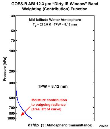
Drag the slider (above) to compare the four Dirty Longwave IR Window band weighting functions.
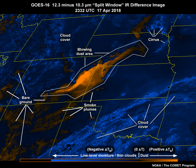
The 12.3 micrometer band also has a long tradition in detecting volcanic ash and airborne dust during daytime and nighttime when combined with an 11 micrometer band. The same processes that enable the detection of thin cirrus are at work within semi-transparent volcanic ash and dust plumes, but in the opposite sense. Ash or dust plumes attenuate less energy at 12.3 than at 10.3 and 11.2 micrometer wavelengths, allowing some of the energy from warmer cloud tops or surfaces below to pass through the plume. This is the reverse of what we saw earlier in the thin cirrus discussion. The effect, often referred to as "reverse absorption", results in a slightly warmer brightness temperature signature in the 12.3 micrometer band when compared to the 10.3 and 11.2 micrometer bands.
Drag the slider to compare longwave IR images with a 12.3 minus 10.3 micrometer "split window" difference image showing a springtime blowing dust event over the High Plains region of the U.S. A visible "red band" image is included for reference.
Drag the slider (above) to compare the five images.
It's obvious from the individual IR bands that the dust signature is more subtle and requires further processing using band combinations to better highlight the airborne dust. While not an optimal product, the 12.3 minus 10.3 micrometer "split window" difference image helps highlight some of the dust signature, shown in shades of orange. Blue shades indicate either larger amounts of low-level moisture or cloud-top features, especially thinner cirrus. We also notice in the lower and left portions of the difference image some orange areas appearing over regions with typically drier and more barren terrain. These signatures can be due to dry sandy soils and even sufficiently thick smoke plumes or other airborne pollutants.
In addition to the moisture, thin cirrus, dust and ash detection applications discussed in this section, the 12.3 micrometer band is a significant contributor to many other GOES-R product categories. Some of these include:
- Surface products where atmospheric moisture corrections are needed
- Cloud products for cloud phase, microphysics, and height
- Stability indices that rely on moisture estimates, and
- Profiles of atmospheric temperature and moisture that continue the legacy of the GOES sounders
Carbon Dioxide (CO2) Band
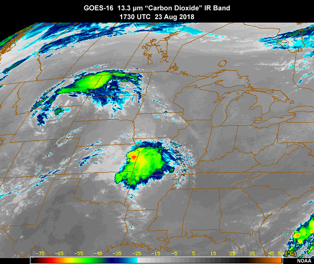
The 13.3 micrometer "carbon dioxide" band is used for a variety of applications including tropospheric temperature and moisture profiles, tropopause delineation, and as part of derived cloud products for cloud opacity estimation, cloud-top height assignments of cloud motion vectors, and supplementing Automated Surface Observing System (or ASOS) observations. Given the complex nature of this band, most applications rely on derived products and not as much on image interpretation.
CO2 bands have been in use for a number of decades now on both GEO and LEO satellites, mainly in support of atmospheric sounding and for assessing cloud-top properties. For GOES satellites, quantitative products have been demonstrated beginning with launch of the GOES-12 satellite in 2001, as well as the GOES sounders beginning with GOES-8 in 1994.
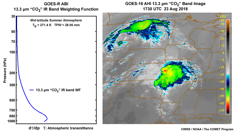
The 13.3 micrometer band is located in the portion of Earth's emitted spectrum where a considerable amount of both cloud and surface radiation is absorbed by carbon dioxide molecules at wavelengths between about 13 and 18 micrometers. Therefore, this band senses radiation from throughout the troposphere. Since carbon dioxide only partially masks clouds and Earth's surface at 13.3 micrometers, the band allows for detection of cloud properties when used in conjunction with other IR window bands.
The weighting function for the CO2 band shown below is for a clear sky U.S. standard atmosphere. The observed brightness temperature can be thought of as a weighted mean value over this pressure range.
Most of the energy originates from middle and lower portions of the troposphere. Since the weighting function peaks near the earth's surface, clouds and surface features are still visible. However, as the contribution to observed brightness temperature due to carbon dioxide becomes more dominant in the lower troposphere, lower clouds and surface features appear less distinct.
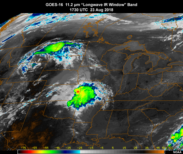
A comparison of 11.2 and 13.3 micrometer band images shows that infrared emission from carbon dioxide partially masks especially the surface and lower cloud features.
Having a dedicated CO2 band on GOES-R at 15-minute intervals over the full Earth disk significantly improves the temporal coverage for derived products compared to the legacy GOES imager's 3-hourly refresh rate.
Imagery and derived products also benefit from the ABI's higher 2-km resolution available to all the IR bands. Higher spatial and temporal resolution allows the ABI to see smaller cloud features and resolve more detailed cloud structure.
Summary
The ABI's expanded suite of longwave IR bands provide forecasters with high spatial and temporal resolution imagery and products for monitoring a variety of surface and atmospheric phenomena. With the addition of new bands, comes significant improvement in the detection and monitoring of cloud-top structures, cloud phase and other microphysical properties, surface features, environmental hazards, and low-level airmass characteristics in the pre-convective environment. The longwave IR bands also help ensure the continuation of legacy atmospheric temperature and moisture profiles important for both nowcasting and short-term forecasts, and further the improvement of cloud motion wind vectors vital to NWP.
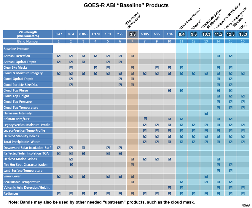
The table below shows the various GOES-R "baseline" products and their reliance on the IR bands presented in this lesson. Based on scientific algorithms, these products provide quantitative information on various physical properties by extracting information from different band groupings known to be sensitive to a specific property.
IR Band Characteristics:
- Spectral Coverage, Bit Depth, Temperature Range
- "Shortwave IR Window" band: 3.9 µm central wavelength, 3.8 – 3.99 μm (GOES-R ABI), Shortwave IR
- Bit Depth: 14 vs. 10 (legacy GOES imager)
- Approximate Maximum Temperature: 410 K (137 °C), about 70 K higher than legacy GOES-13 to -15 imagers
- "Cloud-top Phase" band: 8.4 μm central wavelength, 8.23 – 8.66 μm (GOES-R ABI), Longwave IR
- Bit Depth: 12 vs. 10 (legacy GOES imager)
- Approximate Maximum Temperature: 340 K (67 °C)
- "Ozone" band: 9.6 μm central wavelength, 9.42 – 9.80 μm (GOES-R ABI), Longwave IR
- Bit Depth: 12 vs. 10 (legacy GOES imager)
- Approximate Maximum Temperature: 310 K (-269 to 37 °C)
- "Clean Longwave IR Window" band: 10.3 μm, 10.18 – 10.48 μm (GOES-R ABI), Longwave IR
- Bit Depth: 12 vs. 10 (legacy GOES imager)
- Approximate Maximum Temperature: 340 K (67 °C)
- "Longwave IR Window" band: 11.2 μm, 10.82 – 11.60 μm (GOES-R ABI), Longwave IR
- Bit Depth: 12 vs. 10 (legacy GOES imager)
- Approximate Maximum Temperature: 340 K (67 °C)
- "Dirty Longwave IR Window" band: 12.3 μm, 11.83 – 12.75 (GOES-R ABI), Longwave IR
- Bit Depth: 12 vs. 10 (legacy GOES imager)
- Approximate Maximum Temperature: 340 K (67 °C)
- "CO2" band: 13.3 μm, 12.99 – 13.56 μm (GOES-R ABI), Longwave IR
- Bit Depth: 10 vs. 10 (legacy GOES imager)
- Approximate Maximum Temperature: 318 K (45 °C)
- "Shortwave IR Window" band: 3.9 µm central wavelength, 3.8 – 3.99 μm (GOES-R ABI), Shortwave IR
- Resolution (at equator)
- All infrared bands: 2-km field of view
- Quality Improvements (compared to legacy GOES)
- Less noise
- Higher temperature resolution
- Higher saturation temperatures, and
- Improved pixel geolocation and registration (frame to frame pixel stability)
Application Considerations:
- "Shortwave IR Window" Band
- Available day and nighttime
- Added reflected solar component during daytime results in warmer brightness temperatures
- Products that difference between this band and a longwave IR window band, for low cloud or other water cloud detection for example, are only useful during nighttime
- Band is effective for both day and nighttime cloud phase determination when used in derived products and RGB image composites
- Hot spots and fires: Increased saturation temperature (400 K) allows for improved detection and sub-pixel fire characterization (aerial coverage and burn temperature)
- Increasing noisy brightness temperatures for very cold scenes below -40 C (233 K) during nighttime; affects cirrus, thunderstorm tops, cold wintertime surface scenes
- "Cloud-top Phase" Band
- Available day and nighttime
- Sensitive to low-level moisture, therefore in a "dirty window" band
- Cooler than longwave IR window bands (10.3 and 11.2 µm) for moist low-level air masses and for water clouds
- Warmer than longwave IR window bands for thin cirrus
- Used for estimating cloud-top microphysics (phase and particle size) day and nighttime in conjunction with other IR window bands
- "Ozone" Band
- Available day and nighttime
- Sensitive to upper tropospheric and stratospheric ozone concentrations
- Cooler than IR window bands for cloud-free scenes due to ozone absorption; larger amounts of ozone generally result in more cooling
- Somewhat warmer than IR window bands for clouds near tropopause level due to warming temperatures with height in the stratosphere
- Limited sensitivity to near-surface ozone due to band's broad spectral range
- "Clean Longwave IR Window" Band
- Available day and nighttime
- Cleanest window band with least amount of sensitivity to water vapor
- Provides cleanest view of cloud tops and surface temperature emissions
- Surface temperature and emissivity dominate brightness temperatures in cloud-free scenes
- Slightly warmer than traditional longwave IR window band (10.7 µm on legacy GOES) due to less moisture absorption in lower troposphere
- "Longwave IR Window" Band
- Available daytime and nighttime
- Band that's closest to traditional longwave IR window bands on legacy GOES, Suomi NPP and JPSS
- Brightness temperatures dominated by cloud tops and cloud-free surfaces
- Slightly more sensitive to low-level moisture and therefore cooler than the 10.3 µm clean IR window band
- Slightly cooler than in legacy GOES 10.7 µm IR window band due to greater moisture absorption in lower troposphere
- Slightly cooler semi-transparent cirrus than in legacy GOES 10.7 µm IR window band due to increased absorption of upwelling radiation by ice cloud particles
- "Dirty Longwave IR Window" Band
- Available day and nighttime
- Brightness temperatures dominated by surface temperature and cloud tops
- The most sensitive to low-level moisture compared to other longwave IR window bands
- Coolest of the longwave IR bands due to moisture sensitivity
- Detects thin cirrus, volcanic ash, and airborne dust when used in combination with other IR window bands
- "CO2" Band
- Available day and nighttime
- Sensitive to tropospheric carbon dioxide and somewhat sensitive to water vapor
- Surface and clouds are still visible, however become less distinct at lower levels where carbon dioxide absorption becomes more dominant
- Particularly useful for highlighting higher, colder, and typically ice phase clouds
- Used mainly for derived products and less for image interpretation
- Important input for estimating cloud-top height, temperature and amount
- Important input especially for legacy temperature profiles
You have reached the end of the lesson. Please complete the quiz and share your feedback with us via the user survey.
Resources
Internet Resources
- Official GOES-R Program Site, http://www.goes-r.gov/
- GOES-R Training Overview, http://www.goes-r.gov/users/training.html
- GOES-R: Benefits of Next-Generation Environmental Monitoring, http://www.meted.ucar.edu/training_module.php?id=509
- GOES-R Proving Ground Page, http://www.goes-r.gov/users/proving-ground.html
- GOES-R Documentation Page, http://www.goes-r.gov/resources/docs.html
- GOES-R Scientific Publications, http://www.goes-r.gov/resources/Scipubs/index.html
- GOES and POES Conferences and Meetings, http://www.goes-r.gov/users/conf-mtgs.html
- UW CIMSS Satellite blog and GOES-R, http://cimss.ssec.wisc.edu/goes/blog/archives/category/goes-r
- VISIT: SHyMet for Forecasters: GOES-R 101 Training Session, http://rammb.cira.colostate.edu/training/shymet/forecaster_goesr101.asp
Advanced Baseline Imager (ABI) Specific
- GOES-R ABI Instrument Page, http://www.goes-r.gov/spacesegment/abi.html
- GOES-R ABI: Next Generation Satellite Imaging, http://www.meted.ucar.edu/training_module.php?id=987
- ABI Fact Sheet, http://www.goes-r.gov/education/docs/Factsheet_ABI.pdf
- ABI Bands Quick Information Guides, https://www.goes-r.gov/mission/ABI-bands-quick-info.html
References
GOES-R
- Schmit, T., P. Griffith, M. Gunshor, J. Daniels, S. Goodman, and W. Lebair, 2017: A closer look at the ABI on the GOES-R series. Bull. Amer. Meteor. Soc., 98, 681-698, doi: https://doi.org/10.1175/BAMS-D-15-00230.1.
- Schmit, T.J., S.S. Lindstrom, J.J. Gerth, and M.M. Gunshor, 2018: Applications of the 16 spectral bands on the Advanced Baseline Imager (ABI). J. Operational Meteor., 6, 33-46, doi: https://doi.org/10.15191/nwajom.2018.0604.
- Additional GOES-R and GOES Related Scientific Publications and other documentation (available on the GOES-R Program Site):
Publications: http://www.goes-r.gov/resources/Scipubs/index.html
Documentation: http://www.goes-r.gov/resources/docs.html
Contributors
COMET Sponsors
MetEd and the COMET® Program are a part of the University Corporation for Atmospheric Research's (UCAR's) Community Programs (UCP) and are sponsored by
- NOAA's National Weather Service (NWS)
with additional funding by: - Bureau of Meteorology of Australia (BoM)
- Bureau of Reclamation, United States Department of the Interior
- European Organisation for the Exploitation of Meteorological Satellites (EUMETSAT)
- Meteorological Service of Canada (MSC)
- NOAA's National Environmental Satellite, Data and Information Service (NESDIS)
- NOAA's National Geodetic Survey (NGS)
- National Science Foundation (NSF)
- Naval Meteorology and Oceanography Command (NMOC)
- U.S. Army Corps of Engineers (USACE)
To learn more about us, please visit the COMET website.
Project Contributors
Program Managers
- Wendy Abshire – UCAR/COMET
- Bruce Muller – UCAR/COMET
Project Lead and Meteorologist
- Patrick Dills — UCAR/COMET
Instructional Design
- Bruce Muller — UCAR/COMET
Science Advisors and Contributors
- Dr. Jordan Gerth — Cooperative Institute for Meteorological Satellite Studies (CIMSS)/NOAA/University of Wisconsin
- Tim Schmit — NOAA NESDIS STAR/ASPB @ CIMSS
- Mat Gunshor — CIMSS
Graphics/Animations
- Steve Deyo — UCAR/COMET
Multimedia Authoring/Interface Design
- Gary Pacheco — UCAR/COMET
Audio/Video Editing/Production
- Steve Deyo – UCAR/COMET
Audio Narration
- Vanessa Vincente – UCAR/COMET
GOES-16 Imagery Provided By
- NOAA
Himawari-8 Imagery Provided By
- SSEC/Unidata Community ADDE Open Archive – University of Wisconsin, Madison
- Japan Meteorological Agency (JMA)
COMET Staff, September 2018
Director's Office
- Dr. Elizabeth Mulvihill Page, Director
- Tim Alberta, Assistant Director Operations and IT
- Paul Kucera, Assistant Director International Programs
Business Administration
- Lorrie Alberta, Administrator
- Auliya McCauley-Hartner, Administrative Assistant
- Tara Torres, Program Coordinator
IT Services
- Bob Bubon, Systems Administrator
- Joshua Hepp, Student Assistant
- Joey Rener, Software Engineer
- Malte Winkler, Software Engineer
Instructional Services
- Dr. Alan Bol, Scientist/Instructional Designer
- Tsvetomir Ross-Lazarov, Instructional Designer
International Programs
- Rosario Alfaro Ocampo, Translator/Meteorologist
- David Russi, Translations Coordinator
- Martin Steinson, Project Manager
Production and Media Services
- Steve Deyo, Graphic and 3D Designer
- Dolores Kiessling, Software Engineer
- Gary Pacheco, Web Designer and Developer
- Sylvia Quesada, Production Assistant
Science Group
- Dr. William Bua, Meteorologist
- Patrick Dills, Meteorologist
- Bryan Guarente, Instructional Designer/Meteorologist
- Matthew Kelsch, Hydrometeorologist
- Erin Regan, Student Assistant
- Andrea Smith, Meteorologist
- Amy Stevermer, Meteorologist
- Vanessa Vincente, Meteorologist