Introduction
Introduction » Module Organization
This module will explore the relationships between atmospheric stability, winds, waves, and ocean currents. To do this, we examine the relevant aspects of three case studies: (1) cold season Gulf Stream, (2) cold season Kuroshio Current, and (3) warm season Gulf Stream.
In each case we will examine the relevant aspects of several conceptual topics, including the synoptic setting, ocean currents, evolution of the marine boundary layer (MBL), growth of ocean waves, and potential wave-current interactions. Short background tutorials are available for each topic and are linked to the start of each section of the case studies. They are also available separately under the heading of Background Topics in the menu bar.
Introduction » Objectives
After completing the module, you should be able to do the following:
With regard to Synoptic conditions:
- Identify the synoptic weather pattern that may result in a North Wall event.
- Identify the oceanographic setting that favors a North Wall event.
With regard to the marine boundary layer (MBL):
- Describe the evolution of the MBL during a cold season North Wall event.
- Describe the evolution of the MBL during warm and cold air advection.
- Describe the synoptic and oceanographic conditions that lead to an unstable MBL.
With regard to winds in the MBL:
- Describe how the SST-air temperature difference affects MBL stability.
- Describe how MBL stability affects wind speeds at the surface.
- Describe why NWP models may have difficulty forecasting accurate surface wind speeds during a North Wall event
With regard to ocean waves during a North Wall event:
- List the 3 basic factors that contribute to wave growth.
- Assess the reliability of a model wave forecast using a wave nomogram.
- Assess the reliability of a model wave forecast using ship and buoy observations.
With regard to wave-current interactions:
- Describe the wave-current interactions that increase wave heights.
- Estimate the changes to swell that occur when it runs into an opposing current.
- Describe how waves refract in the presence of current loops and meanders.
- Describe conditions leading to rogue waves.
Introduction » What is a North Wall Event?
Introduction » What is a North Wall Event? » Geography
For narration click the arrow above
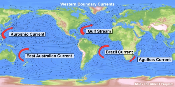
North Wall events refer to high wind and wave events that occur along the north edge of warm, fast, western boundary currents. These events occur along the Gulf Stream off the mid-Atlantic states of the U.S. and along the Kuroshio Current near Japan and Taiwan. Similar events also occur near the Agulhas Current along the east coast of South Africa.
Introduction » What is a North Wall Event? » Hazards
For narration click the arrow above
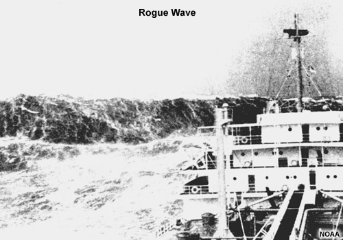
North Wall events present severe challenges and hazards to marine operations. Gale force winds and waves higher than 20 feet regularly occur. Rogue waves are frequently reported during North Wall Events. These rogue waves are thought to occur in response to wave-current interactions.
Introduction » What is a North Wall Event? » Stability, Winds, and Waves
For narration click the arrow above
There are 2 fundamental end-member types of North Wall Events. The first is a cold-season event where a cold air outbreak results in continental Polar air flowing offshore over a warm ocean. The resulting de-stabilization of the lower atmosphere allows high wind momentum to mix to the surface. Ocean waves build quickly in response.
Introduction » What is a North Wall Event? » Wave and Currents
For narration click the arrow above
The other type of North Wall event occurs when ocean swell encounters a current moving in the opposite direction. In response, wave heights increase and the wave period decreases, resulting in taller, steeper waves. More extreme events lead to wave breaking. These events occur in all seasons and may or may not be associated with the cold air outbreaks that typically lead to the first type of North Wall event. The region around the Agulhas Current is particularly prone to high waves resulting from this type of wave-current interaction.
Introduction » Example North Wall Event
Introduction » Example North Wall Event » NAVMETOCCEN-Norfolk North Wall Advisory
For narration click the arrow above
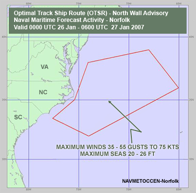
At 00 UTC on 26 Jan 2007, the Naval Meteorology and Oceanography Center at Norfolk, VA issued a North Wall Advisory for the Atlantic Seaboard, with winds of 35-55 kt and maximum seas of 20-26 feet (6-8 meters). These conditions arose from a fairly typical winter North Wall scenario.
UNCLAS //N03144//
MSGID/GENADMIN/NAVLANTMETOCCEN//
SUBJ/OTSR NORTH WALL ADVISORY
UPDATE//
REF/A/NAVLANTMETOCCEN/231921ZJAN2007//
POC/SHIP ROUTING
OFFICER/-/NAVLANTMETOCCEN/LOC:NORFOLK VA/TEL:757-444-7583/EMAIL:
MARITIME.SRO(AT)NAVY.MIL//
RMKS/
1. THIS OTSR NORTH WALL ADVISORY AMENDS REF A TO
REFLECT LATER ONSET OF CONDITIONS DESCRIBED BELOW AND IS NOW EFFECTIVE COMMENCING
260000ZJAN07 AND EXTENDING THRU 270600ZJAN07 FOR AREA DESCRIBED BELOW:
38-00N 74-00W
39-00N 68-00W
36-00N 65-00W
32-00N 74-00W
33-29N 77-35W (FRYING
PAN SHOALS)
35-00N 75-24W (DIAMOND SHOALS)
38-00N 74-00W
WIND/SEAS FORECAST OVER THIS AREA 35 TO 55 GUSTS 75 KNOTS/12 TO 16 FEET WITH MAX OF 20 TO 26
FEET IN THE VICINITY AND EAST OF THE GULF STREAM.
2. BY 25/1200Z A TROUGH OF LOW
PRESSURE TRACKS SOUTHEAST ACROSS THE GREAT LAKES INTO THE ATLANTIC COASTAL WATERS. AS THIS
TROUGH MOVES OFFSHORE IT DEVELOPS INTO A LOW PRESSURE SYSTEM AND TRACKS EAST
INTO THE
WESTERN ATLANTIC WHILE INTENSIFYING. STRONG HIGH PRESSURE OVER THE PLAINS STATES WILL MOVE
EAST-SOUTHEAST AND INTERACT WITH THE OFFSHORE LOW AND ASSOCIATED TROUGH TO PRODUCE A STRONG
NORTHWEST FLOW OFF THE ATLANTIC SEABOARD, ADVECTING ARCTIC AIR (30-40F) OVER THE RELATIVELY
WARMER WATERS (70-75F) OF THE GULFSTREAM. THE VIOLENT INTERACTION OF THIS COLD AIR WITH THE
WARM GULF STREAM WATERS WILL PRODUCE STRONG GALE FORCE WINDS AND HIGH SEAS ACROSS PORTIONS
OF THE VACAPES AND CHERRY POINT OPAREAS. SEAS WILL REMAIN
SIGNIFICANTLY LOWER IN THE
FETCH LIMITED COASTAL WATERS TO THE WEST AND NORTHWEST OF THE GULF STREAM.
3. OTSR
ADVISES ALL UNITS WHOSE LIMITS ARE EXCEEDED BY CONDITIONS DESCRIBED PARA 1, SEEK SAFE HAVEN
IN PORT OR AVOID THIS WARNING AREA UNTIL CONDITIONS ABATE TO ACCEPTABLE LEVELS.
4. OTSR
WILL CONTINUE TO CLOSELY MONITOR THIS EVOLVING WEATHER SITUATION AND ISSUE FURTHER WEATHER
ADVISORIES/DIVERT RECOMMENDATIONS AS CONDITIONS WARRANT.
5. FOR MORE INFORMATION,
CONTACT THE SHIP ROUTING OFFICER USING INFORMATION LISTED ABOVE, OR VISIT OUR WEB SITE AT
HTTP:/WEATHER.NAVY.MIL//
Introduction » Example North Wall Event » NOAA/OPC Storm Warning
For narration click the arrow above
A couple of hours later, NOAA's Ocean Prediction Center issued the following Storm Warning
...STORM WARNING...
...N WALL OF GULF STREAM NEAR 37.5N 72.4W...37.9N 71W...37.7N...69.4W...38N 68.4W...38N 66.9W...
.THIS AFTERNOON...W OF 1000 FMS...NW WINDS 30 TO 40 KT...DIMINISHING TO 25 TO 35 KT LATE.
SEAS 5 TO 10 FT...HIGHEST E OF 1000 FMS...NW WINDS 35 TO 45 KT...EXCEPT TO 60 KT
NEAR AND S OF THE GULF STREAM. SEAS 10 TO 18 FT...EXCEPT TO 27 FT NEAR AND S OF THE GULF
STREAM. SCATTERED RAIN AND SNOW SHOWERS.
.TONIGHT...NW WINDS DIMINISHING
TO 15 TO 25 KT...EXCEPT 25 TO 35 KT E OF 70W...HIGHEST FAR E. SEAS SUBSIDING TO 4 TO 7
FT...EXCEPT TO 20 FT E OF 1000 FMS...HIGHEST FAR E. ISOLATED RAIN AND SNOW SHOWERS.
.SAT...WINDS BECOMING W TO SW 20 TO 30 KT...EXCEPT TO 35 KT NEAR THE GULF STREAM. SEAS
SUBSIDING TO 5 TO 8 FT...EXCEPT TO 15 FT E OF 1000 FMS...HIGHEST FAR E.
.SAT NIGHT...W
TO SW WINDS 25 TO 35 KT EARLY...DIMINISHING TO 15 TO 25 KT. SEAS 4 TO 7 FT...EXCEPT TO 14 FT
E OF 1000 FMS...HIGHEST FAR E. ISOLATED SHOWERS FAR E.
This Marine Weather Discussion accompanied the Storm Warning:
AGNT40 KWNM 261400
MIMATN
MARINE WEATHER DISCUSSION
NWS OCEAN PREDICTION CENTER WASHINGTON DC
836 AM EST FRI 26
JAN 2007
.FORECAST DISCUSSION: MAJOR FEATURES/WINDS/SEAS/SIGNIFICANT .WEATHER FOR NORTH ATLANTIC OCEAN W OF 50W FROM 30N TO 50N. STRONG NW FLOW OVER THE OFFSHORE WATERS THIS MRNG. QUIKSCAT PASS WAS TIMELY...AND SHOWED GALES EXTENDING FM THE S OF NEW ENGLAND WATERS DOWN TO ABOUT CAPE FEAR...THEN SE AND OVER THE NE PORTION OF THE CAPE FEAR TO 31N WATERS. STORM FORCE WINDS ARE IN 50 TO 70 n mi WIDE SWATH EXTENDING FROM NEAR 38.6N 70.4W TO 36.8N 72.8W... AND A SCATTERING OF STORM FORCE WINDS OVER THE E PORTION OF BALT TO HATTERAS CANYON. HIRES QUIKSCAT SHOWS WINDS NEAR HURRICANE FORCE NEAR THE GULF STREAM OVER THE SE PORTION OF HUDSON TO BALT CNYN. QUITE INTERESTING TO NOTE THESE WINDS ARE THE HIGHER THAN ANY WINDS FCST BY THE GFS BELOW 500 MB.
SEAS CLOSE TO THE COAST ARE AVGNG CLOSE TO THE WAVE MODEL... THOUGH FARTHER OUT ARE A GD 10 TO 20 PCT OVER WV MODEL FCST. OVER THE GULF STREAM...SEAS ARE EST TO BE 50 TO 75 PCT HIGHER.
WILL ADJUST WINDS AND SEAS TO CURRENT CONDS...OTW NO SIG CHANGES PLANNED FOR THE FCST UPDATE.
FROM THE PRVS DSCN...
BUOY 41001 RPRTD 35 KT AT 04Z AND 05Z...AND THE RMNDR OF THE LTST
SFC RPRTS INDC STG NW FLOW OVR THE RGN. THE LTST GOES IR IMGRY INDC STG CAA OVR THE MAJORITY
OF THE OFSHR WTRS...AND ALSO A DVLPG LOW E OF THE AREA. THE MDLS ARE INIT OK ON THIS
SYS...AND THE 00Z GFS INDC THAT THE SYS WL MOV NE AND MERGE WITH THE UPR TROF...CRNTLY OVR
THE OFSHR WTRS. THE GFS HAS BEEN CONSISTENT WITH DVLPG THIS SYS QUICKLY...AND THE MDLS ARE
INDCG THAT THE WNDS WL REACH HURCN FRC NE OF THE AREA. OVR THE OFSHR WTRS...THE MDLS ARE IN
GD AGRMT WITH THE STG CAA BEHIND THE CDFNT...AND THE GFS MDL SNDGS INDC STG MXG. THE PREV
FCST INDC GALES ACRS THE ENTIRE AREA...WITH STRM FRC WNDS IN THE GULF STRM FM HUDSON TO
HATERAS CNYNS. ATTM CNFDNC IS HIGH WITH THE GUID...SO XPCT NO CHNGS ATTM WITH THE WRNGS IN
THE NEXT 24 HRS.
THE LTST GFS/NAM/GEM MDLS INDC THAT ANTHR SYS WL EJECT OFF THE NE COAST SAT NGT INTO SUN...AND MDLS HAVE BEEN INDCG MRGNL GALE FRC WNDS AHD OF THE ASSOC CDFNT. THE 00Z UKMET HAS TRENDED TWD THE GFS SOLN...SO ATTM FEEL THAT THERE IS ENUF SUPPORT TO START GALES OVR HUDSON TO BALTO CNYN IN THE VCNTY OF THE GLF STRM.
IN THE EXTENDED PD...MOST OF THE MDLS ARE INDCG THAT ANTHR LOW WL MOV OFF THE SE COAST SUN...AND TRACK NE. THE GFS HAS ALSO BEEN INDCG THAT A NRN STRM LOW WL EJECT OFF THE NEW ENGLAND COAST ABT THE SAME TIME...AND BCM THE DOMINANT FEATURE. HOWEVER...THE MAJORITY OF THE GUID...INCLUDING THE 12Z ECMWF AND 00Z UKMET... FAVOR THE SRN STRM LOW AS THE DOMINANT FEATURE. IN ADDITION...THE MAJORITY OF THE 00Z ENSEMBLE MEMBERS FAVOR THE LOW. THE HPC MDL DIAG WAS CONSULTED AND IS IN AGRMT WITH THE STGR SRN SOLN...SO WL LEAN MORE IN THAT DIR FOR THE NEXT PKG. THE PREV FCST FLWD ALNG THOSE LINES...SO XPCT NO MAJOR CHNGS ATTM. OTW WL STAY NR THE GFS IN THE SHORT TERM...BUT CLOSER TO THE ECMWF/UKMET SOLNS IN THE EXTENDED.
SEAS...THE LTST WW3 MDL IS INIT ABT 6 FT LOW OVR THE OFSHR WTRS...SO WL ADJUST THE MDL HIGHER INITIALLY...AND RMNS TOO LOW WITH THE SEAS IN THE STG CAA. THE WW3 MDL IS ALSO TOO LOW WITH THE SEAS IN THE NEXT CAA EVENT ON MON. OTW WL ACCEPT THE WW3 FOR THE RMNDR OF THE FCST.
.WARNINGS...PRELIMINARY. ANY CHANGES WILL BE COORDINATED THROUGH AWIPS 12 PLANET CHAT OR BY TELEPHONE:
.NT1 NEW ENGLAND WATERS...
.GULF OF MAINE...GALE FRI INTO SAT.
.GEORGES BANK...GALE
TDY INTO SAT...AND MON INTO TUE
.S OF NEW ENGLAND...GALE TDY INTO FRI NGT...AND MON
INTO TUE
.NT2 MID ATLC WATERS...
.HUDSON TO BALT CNYN...STORM TDY. GALE FRI NIGHT THRU SAT
NGT...AND MON INTO TUE.
.BALT CNYN TO HATTERAS CNYN...STORM TDY...GALE FRI NIGHT INTO
SAT...AND MON.
.HATTERAS CNYN TO CAPE FEAR...GALE TDY...AND ON MON.
.CAPE FEAR TO
31N...GALE EARLY TDY...AND ON MON.
.FORECASTER KELLS. OCEAN FORECAST BRANCH.
Introduction » Example North Wall Event » Questions
Based on these forecasts and discussions, please answer the following questions:
Question 1
Where do you expect the strongest winds? Highest waves? (Enter your response and select Done.)
Clearly, the area of greatest concern here is near the Gulf Stream. From the NOAA Storm Warning:
And from the NAVMETOCCEN-Norfolk North Wall Advisory
Question 2
Are waves underforecast or overforecast by the models? (Enter your response and select Done.)
In this case, the models appear to be underpredicting both wind and waves. Note this passage in the marine Weather discussion:
SEAS CLOSE TO THE COAST ARE AVGNG CLOSE TO THE WAVE MODEL... THOUGH FARTHER OUT ARE A GD 10 TO 20 PCT OVER WV MODEL FCST. OVER THE GULF STREAM...SEAS ARE EST TO BE 50 TO 75 PCT HIGHER.
Question 3
Why is this occurring? (Enter your response and select Done.)
As to why this is going on, the North Wall advisory provides a brief summary:
Much of this module examines the reasons why THE VIOLENT INTERACTION OF...COLD AIR WITH THE WARM GULF STREAM WATERS WILL PRODUCE STRONG GALE FORCE WINDS AND HIGH SEAS The remainder examines what happens when waves encounter a current with an opposing flow.
Case Study: Gulf Stream - January 2007
Case Study: Gulf Stream - January 2007 » Synoptic Setting
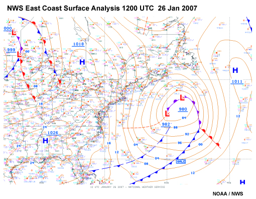
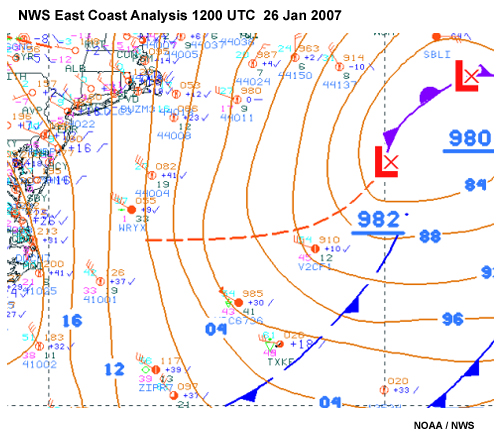
Case Study: Gulf Stream - January 2007 » Synoptic Setting » East Coast Analysis
Background Topic
Question 4
This plot shows the National Weather Service (NWS) Analysis for 1200z 26 January 2007.
What synoptic features are likely to lead to strong offshore winds along the U.S. East Coast? (Enter your response and select Done.)
At this time, a complex low pressure system with a central pressure of 980 millibars was located approximately 500 n mi East of New York City. A deep Canadian Arctic High pressure system at 1026 millibars was located over the Southern USA. A ridge of high pressure extended from northern Mississippi northeastward to southern Quebec. This results in a strong pressure gradient over the coast from Cape Hatteras northward into Canada.
Case Study: Gulf Stream - January 2007 » Synoptic Setting » East Coast Analysis - Zoom
Question 5
Now let's zoom in on the region east of the central Atlantic Seaboard.
How would you characterize winds along the coast? How would you characterize winds offshore? What is the strongest wind you see on this graphic? (Enter your response and select Done.)
Coastal wind observations were recording northwesterly winds at about 15 kt along the shoreline. Observations from buoys located about 100 n mi offshore show winds increased dramatically to about 35-40 kt with waves in the range of 20-30 feet. Clearly the wind and waves increase dramatically as the cold air moves offshore. Notice that one of the ship obs (C6736) is reading 55 kt and 41 ft waves!
This analysis also shows a secondary cold front west of the primary cold front. The secondary cold front reinforced the CAA along the Central Atlantic Seaboard and was associated with an intense short wave trough.
Case Study: Gulf Stream - January 2007 » Synoptic Setting » Ocean Prediction Center (OPC) Analysis
For narration click the arrow above
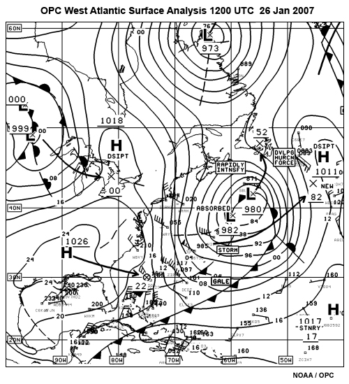
This is the Ocean Prediction Center (OPC) Analysis for 1200 UTC 26 Jan 2007. The OPC is the official source for U.S. Government forecasts along the East Coast for non-DOD assets. This analysis showed a small area of 55 kt winds along and just southeast of the Gulf Stream. Storm force winds (48-63 kt) were being reported by offshore buoys. The high pressure system was forecast to move eastward off the Atlantic Seaboard in the next 24-72hrs.
Beaufort Scale:
Gale = Beaufort_scale 8 or 9: 34-47 kt
Storm =
Beaufort_scale 10 or 11: 48-63 kt
Hurricane = Beaufort scale 12: 64+ kt
Reference:
https://www.weather.gov/mfl/beaufort
Case Study: Gulf Stream - January 2007 » Oceanography
Case Study: Gulf Stream - January 2007 » Oceanography » Gulf Stream Analysis - SST
Background Topic
Question 6
On the image below:
- Use the pen to trace the northern edge of the Gulf Stream (the North Wall) from Florida to where the Gulf Stream Extension leaves the eastern edge of the plot.
When you have finished, select Done.
The Gulf Stream stays along the north side of the temperature gradient between warm and cool colors on the chart.
Compare your answer to the answer below.
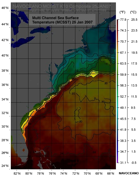
Question 7
In this case study, a northwesterly wind was blowing offshore over the Chesapeake Bay area.
(Enter your responses and select Done.)
Answers: ~10C and >22C
The correct answers are about 10°C close to Chesapeake Bay and about 22°C over the Gulf Stream. Thus, a pronounced SST gradient lies just offshore of the Virginia Capes region. As we discuss later, the rapid increase in SST along the North Wall allows for a large positive vertical flux of energy into the atmosphere and a corresponding downward flux of cold air to the surface of the ocean. The downward momentum flux of cold/dense air leads to significant increases in winds speeds and wave heights downwind from the Gulf Stream.
Case Study: Gulf Stream - January 2007 » Oceanography » Gulf Stream Analysis - Currents
Question 8
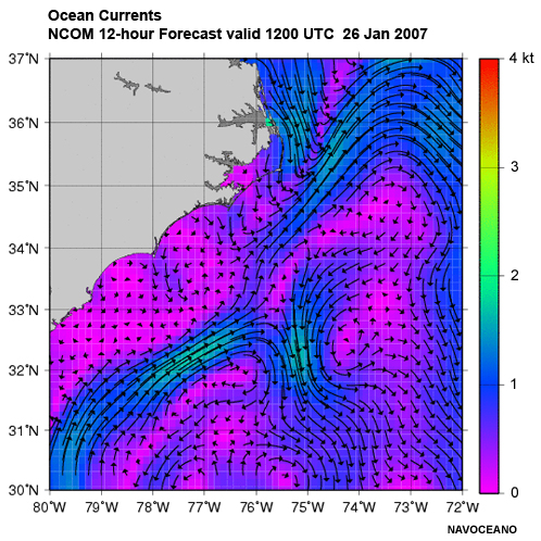
This Navy Coastal Ocean Model (NCOM) 36 hour forecast clearly shows the Gulf Stream.
(Enter your response and select Done.)
The correct answer is 1 to 2 knots.
In general, wave-current interactions increase exponentially as current speed increases and tend to become significant when the current speed exceeds 1 - 1.5 knots. We can see here, that much of the Gulf Stream meets that criteria.
Case Study: Gulf Stream - January 2007 » MBL Stability
Case Study: Gulf Stream - January 2007 » MBL Stability » Coastal Soundings
Background Topic
This sounding comes from Wallops Island, VA, at 1200 UTC on 26-Jan.
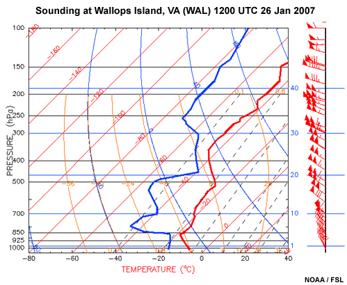
Question 9
How would you characterize the boundary layer? (Enter your response and select Done.)
Here we see a well-mixed boundary layer capped by a stable, isothermal layer just below the 850 hPa level.
Question 10
How would you characterize low level winds? (Enter your response and select Done.)
Wind speeds average 20-30 kt from the surface to 850 hPa and 30-50 kt from the 850 hPa to 700 hPa levels. Winds are uniformly from the northwest at low levels.
Question 11
What do you expect will happen when surface winds advect offshore? (Enter your response and select Done.)
Note that the surface temperature is about -7°C. Offshore SSTs range from 10°C at the coast to over 20°C over the Gulf Stream, setting up a strong SST/air temperature contrast once the cold air moves offshore. Large heat and moisture fluxes should rapidly destabilize and moisten the boundary layer under these circumstances.
Case Study: Gulf Stream - January 2007 » MBL Stability » Coastal Soundings - NWP Models
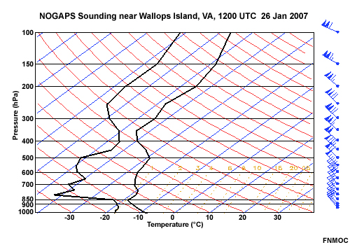
Question 12
Now compare the boundary layer in the observed sounding to the boundary layer in these model soundings from the global NOGAPS model and the North American Mesoscale (NAM) model.
Sounding
NOGAPS
NAM
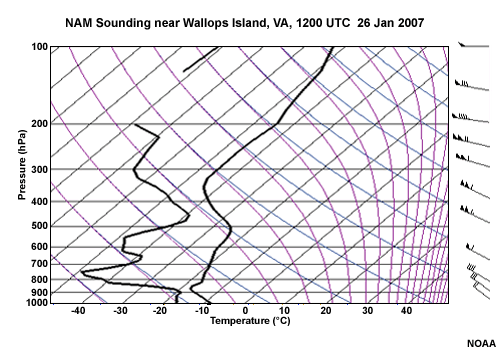
How do the model soundings compare to the observed sounding? (Enter your response and select Done.)
The observed and model soundings are nearly identical. There are no significant differences below 500 hPa. At least over land, NOGAPS and the NAM are performing well.
Case Study: Gulf Stream - January 2007 » MBL Stability » Offshore Air/Sea Temperature Contrast
For narration click the arrow above
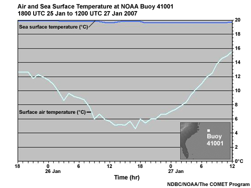
This time series plot shows both air and water temperatures from Buoy 41001, located about 150 n mi east of Cape Hatteras, NC, for this North Wall event. For about a 6-hour period, the air-sea temperature difference was about 15°C. This suggests a strong vertical transfer of heat from the ocean to the atmosphere. Such strong heating quickly destabilizes and deepens the boundary layer.
Case Study: Gulf Stream - January 2007 » MBL Stability » Offshore Sounding - NOGAPS
Question 13
Now look at a NOGAPS sounding for a location near Buoy 41001 at 1200 UTC 26 Jan.
Time series
NOGAPS
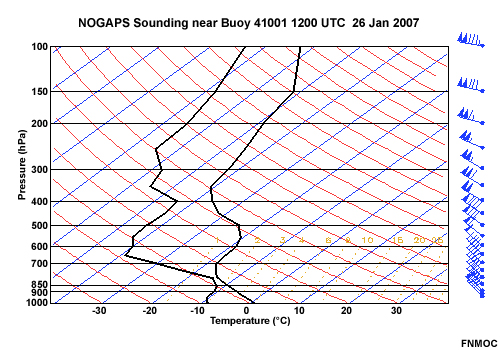
How does the NOGAPS surface air temperature compare to that observed at the buoy at the same time? Choose the best answer.
The correct answer is a) The NOGAPS temperature is colder.
The NOGAPS temperature at the surface is about 1°C, while the air temperature observed at the buoy is about 5°C. It appears that the model is having trouble simulating air temperature near the surface. Without speculating on the cause of this discrepancy, it could have profound implications for boundary layer stability, and subsequently for low-level winds.
Note that the dewpoint profile near the surface shows rapid moistening of the lowest levels. Thus, the model apparently simulates some of the effects of cold air advection over warm water.
Case Study: Gulf Stream - January 2007 » MBL Stability » Offshore Sounding - NAM
Question 14
Now contrast the NOGAPS sounding at Buoy 41001 with the NAM sounding at the same place.
NOGAPS
NAM
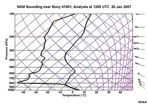
More specifically, how does the boundary layer differ between the two models? (Enter your response and select Done.)
At the surface, the air temperature in the NAM is much warmer than in NOGAPS, and very close to that observed at the buoy. However, the lapse rate is superadiabatic from the surface up to about 850 hPa. Such a deep superadiabatic zone never occurs in nature. The moisture profile is nearly saturated throughout the boundary layer. Surface winds are 35 kt, which agrees well with observations, as we will see later.
So how can the models differ so much, and what does this tell us as forecasters?
When cold outbreaks advect from land out over warm currents,
there are a two major things to consider:
1) What SST information is fed
into the model?
2) How does the boundary layer respond to cold air
advection over warm water?
Global models, like NOGAPS or GFS, have a fairly coarse representation of the Gulf Stream, often derived from climatology. When combined with a large grid spacing, the result may be that the model doesn't "see" the warm water. This may be the source of the cool temperatures in the NOGAPS sounding.
On the other hand, in the NAM, the model mixing may not be fast enough to keep pace with the surface fluxes. The NAM diffuses layer by layer rather than applying an instantaneous mixed profile through the depth of the boundary layer. Thus the upper levels may respond slowly to what is happening at the surface, resulting in a superadiabatic lapse rate.
Also, the NAM has trouble with entraining air above down into the MBL, which can also result in unrealistic soundings. Meanwhile, NOGAPS uses a scheme that is able to entrain air from above down into the MBL. Though its temperature at the surface is too low, the structure of the PBL looks better, and might do a better job of predicting near-surface winds.
One last caveat about model soundings: data processing, such as smoothing or interpolation between grid points, can artificially produce things like superadiabatic layers, particularly in strongly baroclinic situations with a sharp slope to the baroclinic zone. This happens even though the actual model soundings are not superadiabatic.
Case Study: Gulf Stream - January 2007 » MBL Stability » Offshore Sensible Heat Flux
Question 15
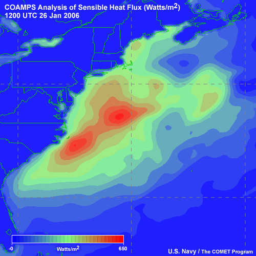
This plot shows the COAMPS Analysis of sensible heat flux at 1200 UTC 26 Jan 2007. Note values associated with the Gulf Stream exceed 600 Watts / m2. These extremely large values rapidly modify the MBL.
Why aren't the highest values further south, where the Gulf Stream is warmer? (Enter your response and select Done.)
Sensible heat flux is the transfer of heat, so it depends primarily on the temperature difference between the sea and air at the surface (evaporation also plays a role, so the relative humidity of the air is also a factor). In this example, we find the greatest sensible heat flux where cold air blows over warm water.
Case Study: Gulf Stream - January 2007 » MBL Winds
Case Study: Gulf Stream - January 2007 » MBL Winds » GOES - 12 (1km) Visible Satellite Picture
Background Topic
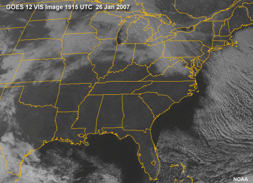
Question 16
The GOES-12 visible picture at 26/1915z shows a pronounced area of cloud free skies along the coast of VA-NC-SC associated with cold / dry air moving offshore. As the air moves further offshore, "clouds streets" begin to form, oriented parallel to the flow.
Given what we know from the synoptic setting for this case, what is the relationship between the spacing between cloud streets and wind speed? Choose the best answer.
The correct answer is a) Tighter spacing = stronger winds.
The closeness of the streets indicates strong winds. The strongest upper level winds are oriented from PIT-DOV-150 n mi East of Cape Hatteras.
Question 17
What determines where the clouds start to form? Choose all that apply.
The correct answers are a) and b).
In response to turbulent convective mixing from the surface up, the MBL deepens and the LCL lowers as cold air advects over warm water. Clouds begin to form where the MBL top and the LCL meet.
Case Study: Gulf Stream - January 2007 » MBL Winds » Quikscat Wind Vectors (26/1800Z)
For narration click the arrow above
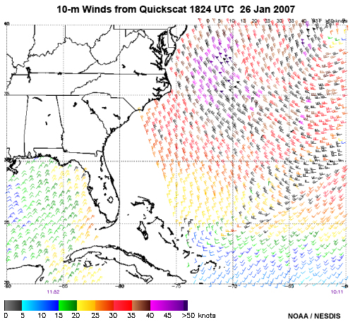
Composite Quikscat imagery at 1824 UTC on 26 January showed an area of strong winds exceeding 35 knots over and south of the North Wall of the Gulf Stream. (The highest reported wind was 55 knots.) The black barbs indicate areas of possible rain contamination. However, very little rain was noted in this area, but banded street clouds were observed.
Case Study: Gulf Stream - January 2007 » MBL Winds » Analysis of Wave Data from Buoy 41001
For narration click the arrow above
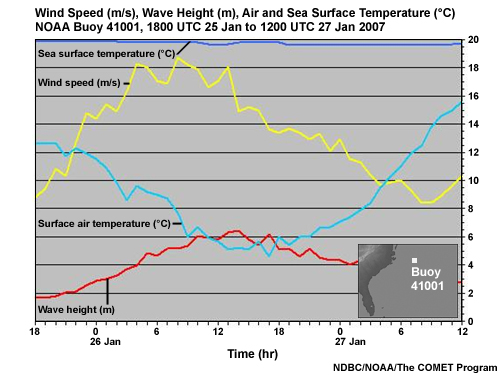
This plot shows a time series of air temperature, SST, wind speed, and wave height from 1900 UTC 25 Jan to 1200 UTC 27 Jan 2007.
During the period from 1800 UTC 25 January until 0400 UTC 26 January (10 hr) the wind speed at Buoy 41001 doubles to over 18 m/s (36 kt) with gusts reported to near 25 m/s (50 kt). Sea heights rose from 2 m (6 ft) to over 6 m (20 ft) over a similar time period. The rapid change in wind speed and sea heights should be questioned to see what “conceptually” is evolving along the Gulf Stream.
Case Study: Gulf Stream - January 2007 » MBL Winds » Model Forecast Winds
For narration click the arrow above
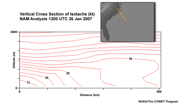
One way to see how winds in the boundary layer are evolving is to construct a cross section of wind speed oriented parallel to the flow. In this case, the cross section extends up to 3000m (10 kft), near the 700 hPa height. At the surface, we see wind speeds increase rapidly as we move offshore, from 8 m/s (16kt) at the coast to 15 m/s (30 kt) about 150 km (80 n mi) offshore over the Gulf Stream.
So why are the winds increasing at the surface? First, let's look at the wind shear. In a truly mixed layer, there should be little wind shear as all the air in a vertical column is moving with the same velocity.
Question 18
Where on this cross section is the least wind shear from the surface up to 1500 m (about 850 hPa)? Choose the best answer.
The correct answer is d) 400 km.
Note that the isotachs over land, near the left side of the cross section, are nearly horizontal and fairly closely packed from 500 to 1500 m. This indicates relatively strong, low-level wind shear. Meanwhile isotachs over the right half of the cross section (over the Gulf Stream) are very steep, in some cases nearly vertical. Where isotachs are steep, wind speed is nearly the same vertically through that layer, indicating little or no wind shear.
Question 19
On the image below:
- Use the pen to draw the top of the MBL on the cross section.
When you have finished, select Done.
Compare your answer to the answer below.
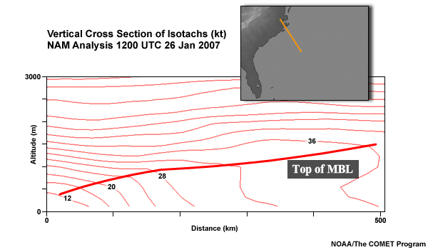
In this cross section, the top of the MBL is marked by the kink in isotachs from horizontal to steeply inclined. The steep isotachs mark a well-mixed column of air with a nearly uniform wind speed. The horizontal isotachs indicate more-stably stratified air with vertical wind shear.
In the context of a cold air outbreak over warmer water, we know that the MBL is destabilizing and deepening as it moves offshore. As the MBL deepens, momentum mixes to the surface from progressively higher levels with higher wind speeds. Thus the increase in wind speed that we see at the surface appears to result from destabilization and deepening of the MBL in response to cold air advection.
Case Study: Gulf Stream - January 2007 » MBL Winds » Wind Speed and Sensible Heat Flux
For narration click the arrow above
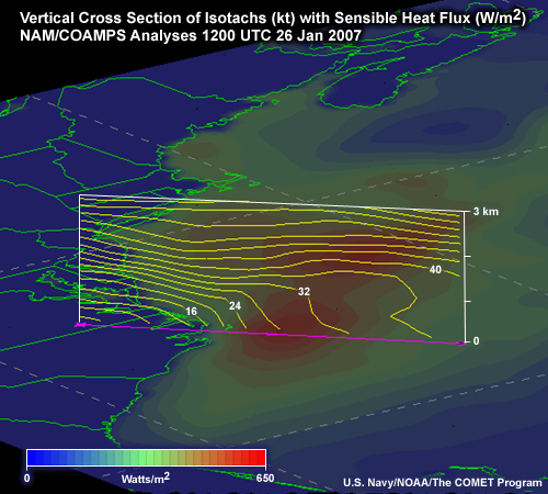
This graphic combines the cross section of isotachs up to 3000m and the map of sensible heat flux. It clearly illustrates the relationship between the deepening of the boundary layer, increased winds at the surface, and high heat flux caused by cold air advection over the warm Gulf Stream.
Case Study: Gulf Stream - January 2007 » Wave Forecast
Case Study: Gulf Stream - January 2007 » Wave Forecast » OPC Wind/Wave Analysis for 26 Jan
Background Topic
For narration click the arrow above
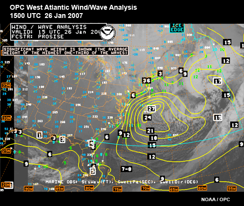
The OPC Wind/Wave analysis shows a 24-27 ft sea height maximum offshore of the Mid Atlantic Seaboard. Note also the 21-foot sea height contour in, near, and downstream of the Gulf Stream. This area of enhanced seas coincides with cloud streets, marine boundary layer instability, and a jet core between 700 and 500 hPa. The destabilized lower atmosphere helps to mix the atmosphere and promote higher wind speeds at the surface, which leads to rapid wave growth.
Case Study: Gulf Stream - January 2007 » Wave Forecast » Analysis of Wave Data from Buoy 41001
For narration click the arrow above
Returning to Buoy 41001, we can see that wave heights reach about 6m (20 ft) for a period of several hours.
Case Study: Gulf Stream - January 2007 » Wave Forecast » Buoy 41001 - 150nm East of Cape Hatteras
For narration click the arrow above
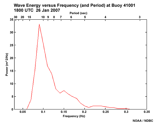
A plot of wave energy versus frequency (and period) shows that MOST of the primary wave energy was focused in the 11 second range at Buoy 41001.
Case Study: Gulf Stream - January 2007 » Wave Forecast » NAVO WAM Model
Now that we've seen what occurred offshore, let's see how the models handled it.
Question 20
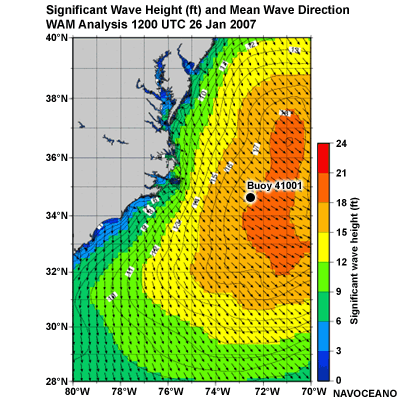
Based on observations at Buoy 41001, how accurate is the NAVO WAM forecast? Choose the best answer.
The correct answer is b) WAM forecast is reasonably accurate.
The NAVO WAM model shows a region of 18-foot seas in the vicinity of Buoy 41001. This is only about 10% lower than the observed wave height.
Case Study: Gulf Stream - January 2007 » Wave Forecast » FNMOC Wavewatch III (WWIII)
Now how does the Wavewatch III handle the forecast?
Question 21
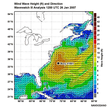
Based on the OPC Wind/Wave analysis, how accurate is the Wavewatch III forecast? Choose the best answer.
The correct answer is a).
Wavewatch III significantly underforecasts wave heights. The Wavewatch III model predicts wave heights of 15 to 18 feet, about 33% below the maximum heights of 24 to 27 feet that we saw in the OPC analysis.
Case Study: Gulf Stream - January 2007 » Wave Forecast » Wavewatch III with Satellite Altimetry Overlay of Wave heights
For narration click the arrow above
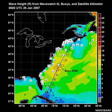
However, at 0600 UTC, the Wavewatch III forecast appeared to be in relatively close agreement with buoy observations and satellite estimates.
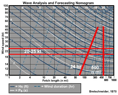
Case Study: Gulf Stream - January 2007 » Wave Forecast » Wave Forecast from the Wave Nomogram - Fetch
For narration click the arrow above
Another way to verify a model forecast is to determine the swell height and period using a wave nomogram. If the model forecast agrees with observations, then we gain some more confidence that the wave forecast is sound.
To determine wave heights, we need to know the fetch, wind speed, and wind duration. We'll use model winds, just like the wave model. Then, we'll compare the results to wave observations at Buoy 41001, 150 n mi east of Cape Hatteras.
Question 22
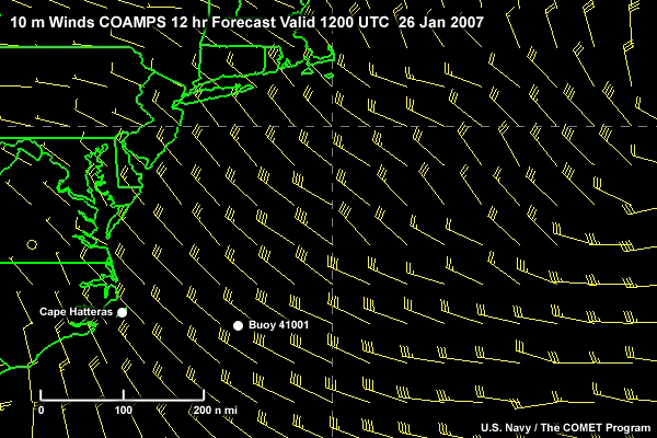
Using this plot of 10-meter winds from the COAMPS 12-hour forecast, what is the fetch for waves observed at Buoy 41001? Choose the best answer.
The correct answer is c) 200 n mi.
Looking at the map, we draw the fetch parallel to the wind direction from the buoy back to the coast. If the buoy is 150 n mi from Cape Hatteras, then the fetch, in this case is somewhat longer, 200 n mi.
Case Study: Gulf Stream - January 2007 » Wave Forecast » Wave Forecast from the Wave Nomogram - Wind Speed
Question 23
Now, using the same plot, what wind speed should we use for our wave determination? Choose the best answer.
The correct answer is b) 30 kt.
This plot indicates that winds at the buoy are about 35 kt. However, over the length of the fetch, winds increase from 25 kt near the coast, to about 35 kt near the buoy. Thus, a better number for wind speed is probably 30 kt, rather than 35 kt.
Case Study: Gulf Stream - January 2007 » Wave Forecast » Wave Forecast from the Wave Nomogram - Wind Duration
Now, how about wind duration? This can be estimated in several ways, including examination of a loop of near-surface winds or examination of a time series plot. In this case we will use the time series plot of winds observed at the buoy.
Question 24
For what duration prior to 1200 UTC 26 Jan do wind speeds exceed 30 kt at Buoy 41001? Choose the best answer.
The correct answer is b) 12 hours.
Winds first exceeded 30 kt at about 00 UTC on 26 Jan. Thus the duration is about 12 hours. If we wish to be a bit more liberal, we can see that winds exceed 20 kt starting about 1930 UTC on 25 Jan. this would yield a wind duration of about 16 hours, but includes weaker winds to start that time period.
Case Study: Gulf Stream - January 2007 » Wave Forecast » Wave Forecast from the Wave Nomogram - Wave Height and Period
Question 25
So now we can apply the wind speed, duration, and fetch to the wave nomogram.
Wind speed = 30 kt
Wind duration = 12 hr
Fetch = 200 n mi
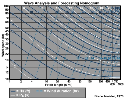
Based on this information, what wave height and period do you expect at the buoy? Choose the best answer.
The correct answer is a) 11 feet.
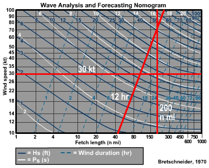
To properly use the nomogram, we first start in the lower-left corner. Then we slide up the vertical axis to the horizontal 30 knot line. From there, we move right until we come to either the 12-hour wind duration or the 200 n mi fetch, whichever comes first. In this case, we first encounter the 12-hr line. The intersection of the 30 kt line and the 12-hr line indicates a wave height of 11 feet with a period of about 7.5 seconds. Note that because we encounter the time line first, the wave height is duration limited.
If we had encountered the fetch of 200 n mi first, wave heights would be fetch-limited. In this case, the wave height would have been 14 feet with a period of 8.3 seconds. Recall that we observed a wave height of 20 feet and a period of 11 seconds at Buoy 41001 at this time.
So what does this mean for our forecast? The simplest interpretation is that COAMPS underforecast the winds. Since the fetch and wind duration are constrained by observations, we can reasonably deduce that COAMPS underforecast the wind speed. Using the nomogram, we can infer a wind speed of approximately 40 kt for a duration of about 15 hours, given a fetch of about 200 n mi.
Another interpretation might arise from wave-current interactions in the vicinity of the Gulf Stream. Swell encountering loops and meanders in the Gulf Stream as it detaches from the coast may be refracted in such a way as to focus wave energy, resulting in higher waves with a longer period.
Case Study: Kuroshio Current - March 2006
Case Study: Kuroshio Current - March 2006 » Synoptic Setting
Case Study: Kuroshio Current - March 2006 » Synoptic Setting » Siberian Cold Air Outbreaks
Background Topic
For narration click the arrow above
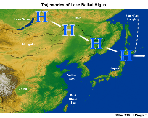
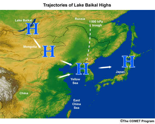
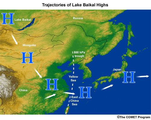
During the Asian winter, a vast, shallow continental polar (cP) air mass forms in the interior of Siberia, leading to a thermal anti-cyclone know as the Siberian High. Central pressure under the Siberian High can range between 1045 hPa to 1065 hPa in the deep of winter with surface temperatures ranging from -9°C to -40°C. Migratory highs develop in the vicinity of Lake Baikal and are known as Lake Baikal Highs. Cold air outbreaks occur when these highs move out of their source regions through Mongolia or northeast China. Thes images show the typical trajectories of highs that form to the northeast, east, and west of Lake Baikal. When they arrive at the coast, the resulting cold surges can bring long-duration gale to storm force winds and high seas to parts of Korea, Japan, southeastern China, and the northern Philippines.
Case Study: Kuroshio Current - March 2006 » Synoptic Setting » West Lake Lake Baikal High and Cold Surge outbreaks
For narration click the arrow above
Of the 3 identified trajectories for cold air outbreaks, the West Lake Baikal High is most likely to bring arctic air to large portions of Asia. After it breaks off from the main Siberian High, it typically moves southeast into China, then east into the East China Sea, and finally northeast to pass south of Japan. On average, these highs occur three to four times a month and typically follow on the heels of arctic air masses and fronts.
Stronger highs lead to stronger northwest winds, significant cold air advection, heavy snow in mountain areas, and a significant buildup of seas that can block ports for days at a time.
Case Study: Kuroshio Current - March 2006 » Synoptic Setting » MSLP During West Baikal Outbreak
For narration click the arrow above
Surface charts will show a strong, closed, high pressure system which generally moves southeast over time while cyclogenesis occurs in the Yellow Sea or the Sea of Japan. Development of a low aids in tightening the pressure gradient.
Strong northwesterly gale and storm force winds follow passage of the arctic front and the development of low pressure in the East China Sea. The resulting high seas limit or restrict marine activity for 36-48 hours.
Case Study: Kuroshio Current - March 2006 » Synoptic Setting » Satellite Signature
For narration click the arrow above
As this satellite loop shows, cold air streams offshore following frontal passage and cloud streets develop. Over the next several hours, these cloud streets coalesce into extensive regions of low stratus.
Case Study: Kuroshio Current - March 2006 » Oceanography
Case Study: Kuroshio Current - March 2006 » Oceanography » Kuroshio Current
Background Topic
For narration click the arrow above
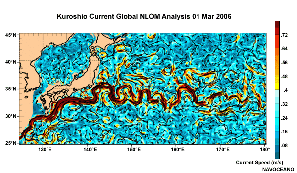
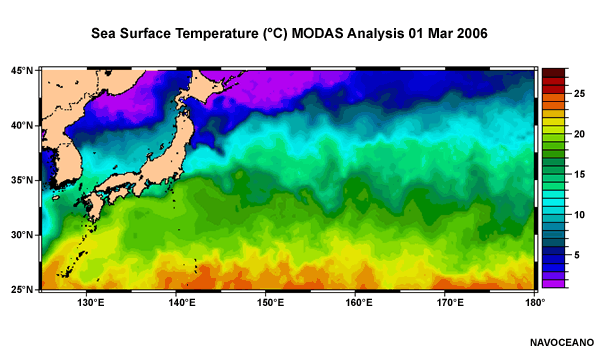
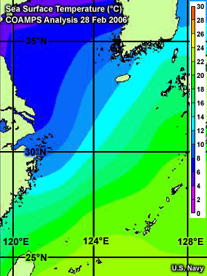
Like the Gulf Stream, the Kuroshio Current is a strong western boundary current. These plots show SSTs and currents for the Kuroshio Current at 00 UTC 1 March 2006.
Question 26
NLOM
MODAS
How would you characterize the Kuroshio Current near Japan?
Use the pull-down menu to choose the best answer.
The correct answers are highlighted above.
Like other western boundary currents, the Kuroshio Current brings warm water from the tropics to mid-latitudes. As a result, Siberian cold air outbreaks lead to North Wall events with high winds and high seas.
Case Study: Kuroshio Current - March 2006 » Oceanography » The Kuroshio Current in COAMPS
Question 27
Compare this MODAS analysis of SSTs with the SSTs used by COAMPS for the same time. How do they differ? (Enter your response and select Done.)
The main difference between the MODAS and COAMPS SSTs is that the COAMPS SSTs are much more smoothed and fail to show strong temperature gradients and the fine details of the temperature distribution. This occurs because the COAMPS SSTs are based upon climatology, which smooths over the strong temperature gradients that exist along the Kuroshio Current. The COAMPS model analysis of SST does not provide detailed resolution of the North Wall of the Kuroshio Current between Kyushu and Okinawa. As a result, boundary layer stability and winds in the model simulation may differ from those observed.
Case Study: Kuroshio Current - March 2006 » MBL Stability
Case Study: Kuroshio Current - March 2006 » MBL Stability » Air/Sea Temperature Difference
Background Topic
Question 28
NOGAPS
NCODA
If we compare air temperature at the surface with sea surface temperatures over the Kuroshio Current in the vicinity of Okinawa, what do we see? Choose the best answer.
The correct answer is e) Air temperature 20°F colder that SST.
The Kuroshio Current near Okinawa has a water temperature over 70°F, while the air temperature is about 50°F, so the air is about 20°F colder than the water.
Question 29
Use the pull-down menu to choose the best answer.
The correct answer is highlighted above.
An air temperature 20°F colder than the water should act to destabilize the MBL.
Case Study: Kuroshio Current - March 2006 » MBL Stability » MBL Evolution along a Trajectory
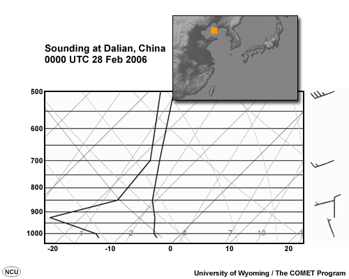
Question 30
This sequence of soundings roughly follows the trajectory of an air parcel near the surface. Each sounding is 24 hours apart.
Dalian, China
Cheju, Korea
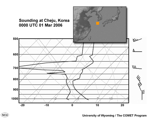
Naze, Japan

Select the correct words to complete the sentence.
The corrects answer is that the MBL becomes less stable, deeper, warmer, and moister as it advects over increasingly warmer water. Air temperature near the surface rises from -5°C to nearly 10°C. The top of the MBL rises from very near the surface to above the 750 hPa level and saturates. Low-level lapse rates increase, indicating destabilization of the MBL.
Case Study: Kuroshio Current - March 2006 » MBL Stability » MBL Evolution at a Point
Question 31
This sequence of soundings was taken at Naze over a 24-hour period.
00 UTC 01 Mar 2006
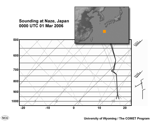
12 UTC 01 Mar 2006
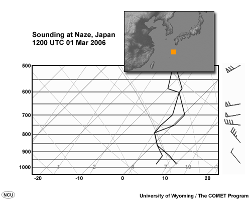
00 UTC 02 Mar 2006
Select the correct words to complete the sentence.
The corrects answer is that the MBL becomes less stable, deeper, cooler and drier over time. The initial MBL is fairly warm and saturated. With cold air advection, the surface air temperature drops from 15°C to about 8°C and an unstable MBL develops and deepens. Near-surface conditions, however, dry out with time: dewpoint depression increases from 1°C to over 5°C throughout the period.
Case Study: Kuroshio Current - March 2006 » MBL Stability » Model versus Observed Sounding
Question 32
Compare these model and observed soundings for 00 UTC 2 March 2006 for Okinawa, Japan.
Sounding
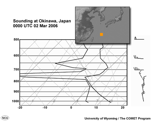
COAMPS
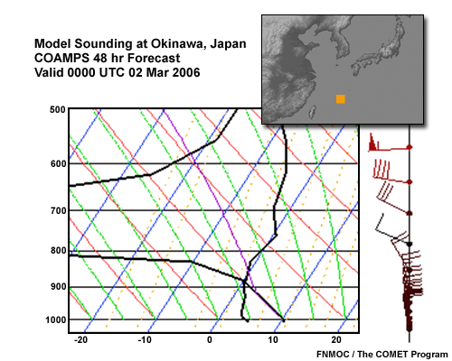
What is the single largest discrepancy between the two soundings? (Enter your response and select Done.)
The biggest difference between the two soundings is the depth of the MBL. Note that the model sounding shows an adiabatic (unstable) lapse rate from the surface to about 880 hPa, while the MBL in the observed sounding extends from the surface to nearly 750 hPa. Under some circumstances this could limit winds mixing to the surface and lead to an underforecast of wind speed. However, in this case, boundary layer winds appear similar in both of the soundings.
Case Study: Kuroshio Current - March 2006 » MBL Winds
Case Study: Kuroshio Current - March 2006 » MBL Winds » Review of SSTs
Background Topic
For narration click the arrow above
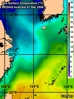
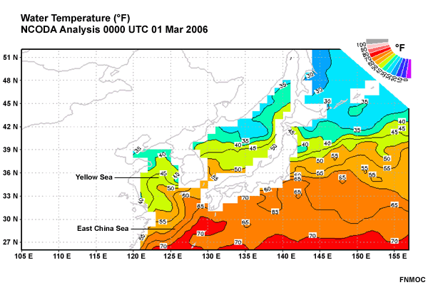
Recall that in the western Pacific, the northeastward-flowing Kuroshio Current results in very warm SSTs with a large temperature gradient near the coast. In the case we are following here, cold winds blow down the Yellow sea into the East China Sea. Along this trajectory, SSTs rise from 35°F in the northern Yellow Sea to over 70°F in the Kuroshio Current.
Case Study: Kuroshio Current - March 2006 » MBL Winds » Evolution of the Wind Field
Question 33
This loop of MSLP and winds shows how wind speed changes as cold air advects along its trajectory from cooler to warmer SSTs.
00 UTC 28 Feb 2006, East Asia
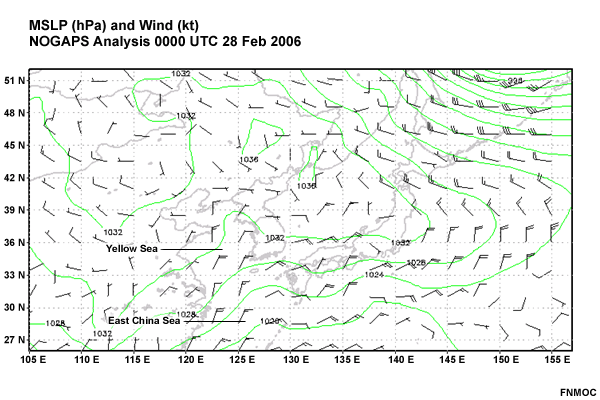
12 UTC 28 Feb 2006
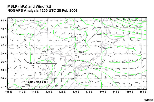
00 UTC 1 Mar 2006
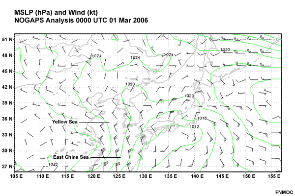
What is the average wind speed over the East China Sea at each time? Use the pull-down menu to choose the best answer.
The correct answers are highlighted above.
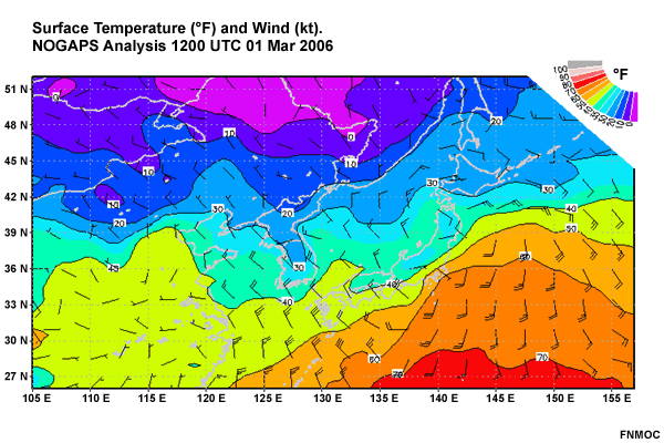
The wind speed increases through the period from about 15 kt to 25-30 kt. This increase in wind speed is driven by both a tightening pressure gradient at the surface and momentum mixing from above in response to deepening of the MBL.
Case Study: Kuroshio Current - March 2006 » MBL Winds » Vertical Structure of the Wind Field
Question 34
This loop shows winds from the surface to 700 hPa at 12 UTC 01 Mar 2006.
MSLP (hPa) and Wind (kt)
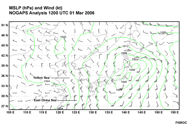
850 hPa Height (m) and Wind (kt)
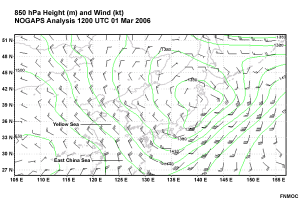
700 hPa Height (m) and Wind (kt)
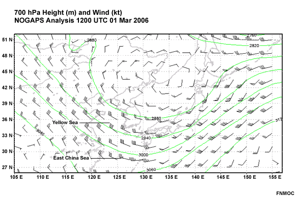
In this table, fill in values for average wind speed over the northern Yellow Sea and the central East China Sea. (Enter your responses and select Done.)
In the northern Yellow Sea, wind speed increases from 15 kt at the surface to over 30 kt at 700 hPa. By the time the wind reaches the Kuroshio region in the East China Sea, winds are consistently 25-35 kt from the surface up to 700 hPa. Deepening and destabilization of the MBL allows stronger winds to mix downward from aloft, resulting in stronger winds at the surface and less wind shear.
Because the default data display is rarely a cross section, we frequently need to examine several map view plots to determine the vertical structure of the atmosphere. Typically, some of the detail is lost when you only see information at significant levels (1000 hPa, 925 hPa, 850 hPa, and so on), particularly in the boundary layer. However, if you have an idea of what may be going on, you should be able to gather enough evidence to confirm or deny your hypothesis.
Case Study: Kuroshio Current - March 2006 » Wave Forecast
Case Study: Kuroshio Current - March 2006 » Wave Forecast » 00 UTC 28 Feb 2006
Background Topic
For narration click the arrow above
Surface Winds
Wave Direction
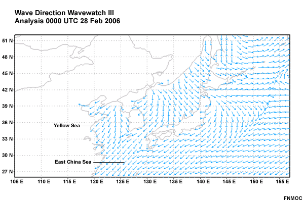
Wave Height
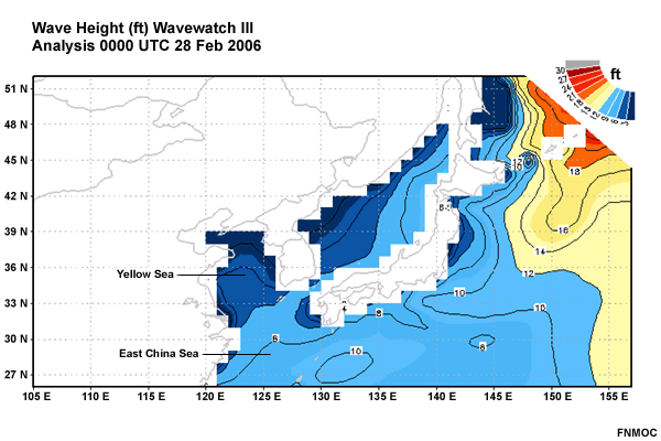
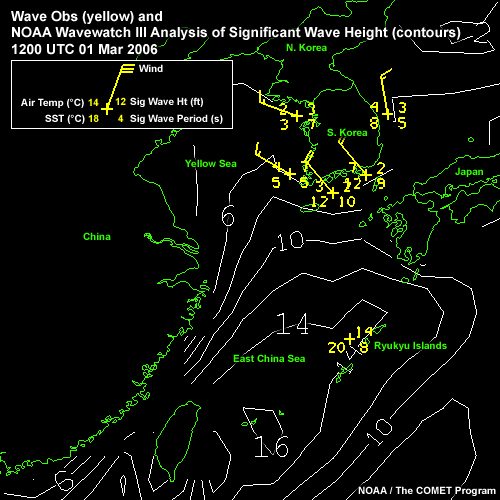
Let's start the wave forecast by reviewing conditions at 00 UTC 28 Mar 2006, before cold air advection affected the offshore region. An analysis of wave direction shows that wind waves build in the Yellow Sea in response to north-northeast winds behind the front. Wave heights range from 3-6 ft in the Yellow Sea due to the northeast winds.
Case Study: Kuroshio Current - March 2006 » Wave Forecast » 00 UTC 01 Mar 2006 - 24 Hours Later
For narration click the arrow above
Surface Wind
Wave Height
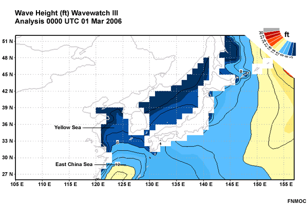
By 00 UTC 01 Mar 2006, winds have strengthened over the East China Sea to 25-30 kt. Winds have also shifted slightly around to the northwest in the Yellow Sea and north in the East China Sea.
In response to the increased wind speed and wind duration, wave heights build in the East China Sea.
Case Study: Kuroshio Current - March 2006 » Wave Forecast » 12 UTC 01 Mar 2006 - 12 Hours Later
For narration click the arrow above
Surface Wind
Wave Height
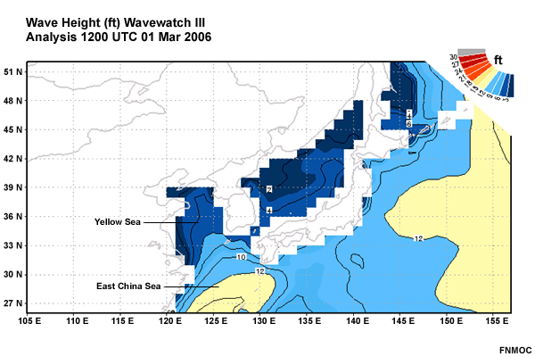
Twelve hours later, wind waves build in the Yellow Sea and expand southward into the East China Sea. Wavewatch III shows 12-14 ft seas with wave periods of 11-13 seconds. This is NOT a North Wall effect, just an ordinary development and movement of wind waves after a cold air outbreak from the Yellow Sea.
Case Study: Kuroshio Current - March 2006 » Wave Forecast » Evaluating the Model Wave Forecast - Winds
For narration click the arrow above
In order to evaluate the reliability of a wave model forecast, we need to compare it to observations at the analysis time. Specifically, we need to see if the winds that force the waves are reasonably well forecast.
Question 35
Here we see a loop of surface winds in the Yellow Sea and East China Sea during the North Wall event. Wind barbs in yellow were observed at ships and buoys. Cyan wind barbs show the GFS Analysis.
During this period how do the GFS analysis winds compare to the observed winds? Choose the best answer.
The correct answer is b).
Early in the event, it appears that the GFS was underforecasting winds along the western side of the East China Sea. This tendency decreased with subsequent analyses. Elsewhere in the forecast area, GFS winds tend to agree reasonably well with the observed winds.
Case Study: Kuroshio Current - March 2006 » Wave Forecast » Evaluating the Model Wave Forecast - Wave Height
Question 36
Now compare the Wavewatch III wave analysis to the observed wave heights. At each station on these graphics, the wave height (in feet) is given by the number located to the upper-right of the small cross.
During this period how do the analyzed Wavewatch III wave heights compare to the observed wave heights? Choose the best answer.
The correct answer is b) Wavewatch III wave heights reasonably match observed waves.
In general, the model wave heights agree reasonably with the observed wave heights. Note however, that early in the period (1200 UTC 28 Feb), when winds were underforecast, that the observed wave heights in the East China Sea significantly exceed the model analysis. Also note that late in the period, the observed wave heights near the Ryukyu Islands are somewhat smaller than the model analysis wave heights.
Case Study: Kuroshio Current - March 2006 » Wave Forecast » Using the Wave Nomogram to Evaluate the Model Wave Forecast - 1
There will be times when pertinent wind and wave observations are simply not available to compare against model predictions. In these cases, it helps to determine wave heights using a wave nomogram in order to evaluate the model forecast.
Question 37
Let's consider a case for the East China Sea near Okinawa at 1200 UTC 1 Mar 2006.
In the graphics of this loop, lines of latitude and longitude are drawn every 5 degrees. 5 degrees of latitude spans about 300 n mi.
Based on this image loop, what would be appropriate values for wind speed, wind duration, and fetch for use with the wave nomogram? (Enter your responses and select Done.)
The appropriate values are:
Wind speed = 20-25 kt
Wind duration = 24 hr
Fetch = about 500 n mi
Case Study: Kuroshio Current - March 2006 » Wave Forecast » Using the Wave Nomogram to Evaluate the Model Wave Forecast - 2
Question 38
Using a Wind speed of 20-25 kt, duration of 24 hr, and fetch of 500 n mi, what wave height would you expect in the East China Sea near Okinawa (Enter your response and select Done.)
In the range of 20-25 kt, we can expect wave heights of 8-10 feet at 24 hours. With a fetch of 500 n mi, waves would grow larger, but that would require a wind duration of about 48-60 hours.
At 1200 UTC on 1 March, both the wave model and the observations indicate a wave height of about 14 feet. On the nomogram, this would require a wind speed of about 30 kt for a duration of 24 hours. This result indicates that either winds were slightly higher than forecast, or that some of the conditions for use of the wave nomogram were not satisfied, so that the wave nomogram underpredicted wave heights.
Case Study: TC Florence - September 2006
Case Study: TC Florence - September 2006 » Synoptic Set-up
Background Topic
Question 39
This is the Ocean Prediction Center (OPC) surface analysis from 1200 UTC 11 Sep 2006. Remember that the OPC is the official source for U.S. Government forecasts along the East Coast for non-DOD assets.
What synoptic features are likely to lead to high seas along the U.S. East Coast? (Enter your response and select Done.)
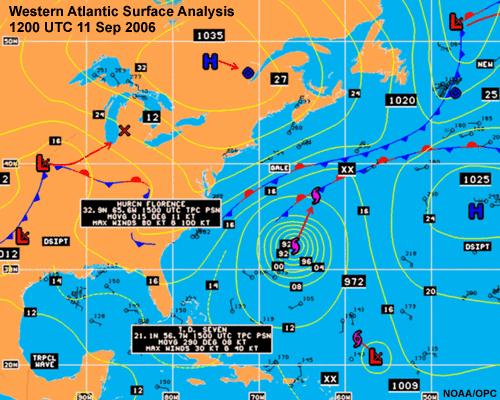
The OPC surface analysis shows two main features: Tropical Cyclone (TC) Florence over the subtropical Atlantic and a 1035-hPa high pressure system over Quebec, Canada. Florence was moving north-northeastward at 11 knots with maximum winds of 80 knots with gusts to 100 knots. The high was moving east southeastward toward the Canadian Maritime provinces of Nova Scotia and Newfoundland.
The interaction of the hurricane and the high pressure system was producing a long fetch of 25-30 knot winds that extended from Newfoundland southwestward to Cape Hatteras and Northern Florida. The fetch length was approximately 1200 n mi long by 200 n mi wide. The large fetch and strong winds are likely to lead to high seas along the U.S. East Coast.
Case Study: TC Florence - September 2006 » Wind / Wave Analysis
For narration click the arrow above
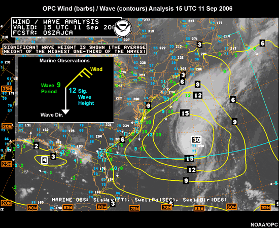
The wind and wave analysis from OPC shows surface observations and contoured significant wave heights over an IR satellite image. A large area of 9-12 foot seas was observed over much of the East Coast.
Case Study: TC Florence - September 2006 » Satellite Analysis
Question 40
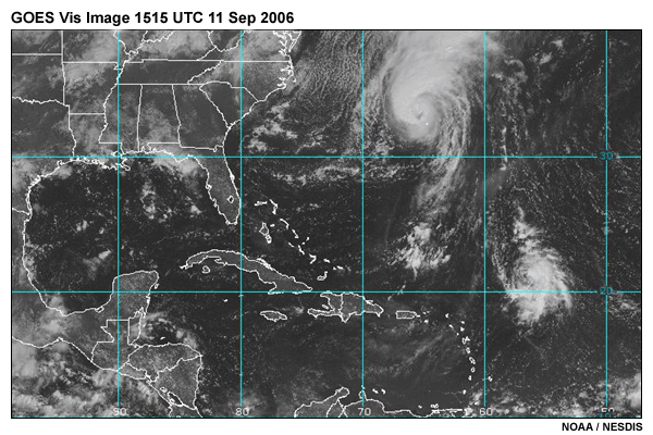
In this GOES East visible satellite image, what clues do we see for the strength and direction of the wind along the U.S. East Coast? (Enter your response and select Done.)
Offshore Cape Hatteras, the presence of cloud streets and open-cell cumulus indicates strong surface winds out of the north-northeast.
Case Study: TC Florence - September 2006 » QuikScat Winds
For narration click the arrow above
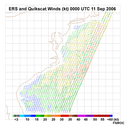
Consistent with the analysis of the GOES Visible image, ERS and Quikscat vectors showed sustained north-northeasterly winds of 20-25 knots from Cape Cod down past Cape Hatteras.
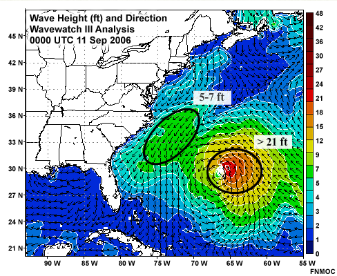
Case Study: TC Florence - September 2006 » Wavewatch III Forecast - 1
Question 41
This plot shows the Wavewatch III (WWIII) analysis at 00 UTC 11 Sep 2006.
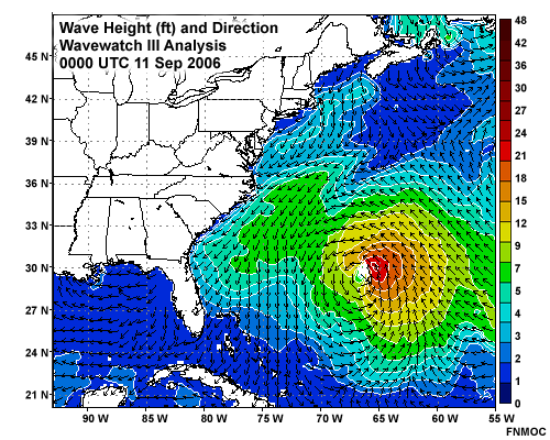
At this time, how large are the waves over the North Wall of the Gulf Stream? Choose the best answer.
The correct answer is a) 5 to 7 ft.
At 00 UTC 11 Sep 2006, Wavewatch III was showing 2 distinct wave areas over the Western Atlantic. Area 1 was associated with TC Florence with wave heights of 21-24 ft in a small core in the right-front (NE) quadrant of the storm. Area 2 was located in the vicinity of the Gulf Stream and was associated with the northeast wind fetch along the Eastern Seaboard. Wave heights in this area were 5-7 ft at this time.
Question 42
Buoy 41001, located 150 n mi east of Cape Hatteras, NC, reported the following conditions at 00 UTC 11 Sep 2006:

Does Wavewatch III reflect the observed wave heights in Gulf Stream near the North Wall? Choose the best answer.
The correct answer is b) No.
While Wavewatch III is predicting seas of 5-7 feet, the measured wave height (WVHT in the table) is 3 meters (10 feet), an underforecast of 50-100%. While the exact cause for this poor model performance is unknown, this is a situation where strong wave-current interaction would act to increase wave heights and shorten wave periods.
Case Study: TC Florence - September 2006 » Wavewatch III Forecast - 2
Question 43
This plot shows the Wavewatch III (WWIII) analysis 24 hours later, at 00 UTC 12 Sep 2006.
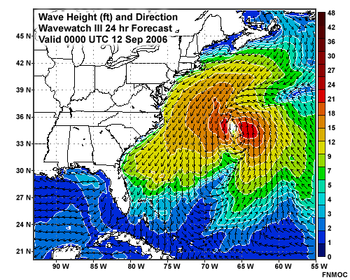
At this time, how large are the waves over the North Wall of the Gulf Stream? Choose the best answer.
The correct answer is b) 12-15 ft.
24 Hours later, WWIII shows a large increase in wave heights along the Eastern Seaboard. Wave heights on the eastern half of Hurricane Florence stayed in the 21-24 ft range but SIGNIFICANT wave building occurred in the western quadrant as the storm grew in size. Wave heights over the North Wall grew to 12-15 ft, and increased to 15-18 ft further offshore.
Question 44
Buoy 41001 reported the following conditions at this time:

Use the pull-down menu to choose the best answer.
The correct answers are highlighted above.
The Wavewatch III forecast of 12-15 foot seas agrees closely with observations at Buoy 41001 of 4.18 m seas (about 14 feet).
Recall that rogue waves can result from wave refraction when swell encounters strong, curved currents. Recall as well that the Gulf Stream loops and meanders once it leaves the coast and moves offshore. In this case, we have large swell coming into the North Wall region from the north-northeast, the most likely scenario for rogue waves.
Case Study: TC Florence - September 2006 » OPC Wind and Wave Forecast
For narration click the arrow above
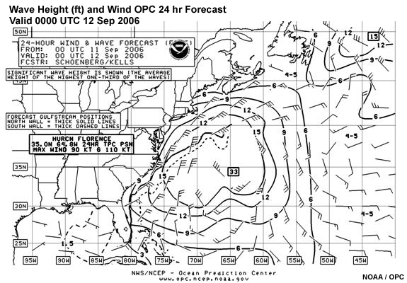
This OPC 24-hr Wind and Wave Forecast for the Western Atlantic also shows the position of the Gulf Stream. The North Wall of the Gulf Stream is shown as a THICK solid line. The south wall is a thick dashed line. From the wind direction, we can see that swell will be moving in a direction almost directly opposed to the current. The winds are forecast to be north-northeasterly at 35 kt with wave heights over 15 ft across a broad area off the Eastern Seaboard.
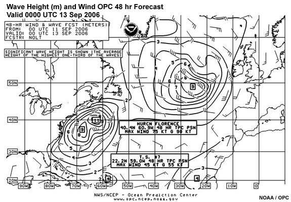
The OPC 48-hr wind and wave forecast for the North Atlantic shows winds continuing to be north-northeast at 20-25 kt with wave heights in the 6-9 meter range (18-27 ft) in the vicinity of the North Wall. This clearly demonstrates that North Wall events can persist for days with the case of a slow-moving tropical cyclone positioned off the eastern U.S.
Case Study: TC Florence - September 2006 » High Winds and Seas Warning
For narration click the arrow above
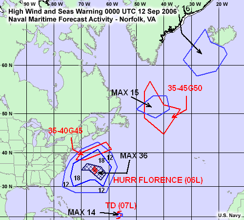
The 00Z 12 Sept 2007 High Winds and Seas message from the Norfolk Marine Forecast Center (NMFC) shows an 18 ft sea height contour for the North Wall area.
Summary
For narration click the arrow above
Cold season North Wall events typically start with some sort of cold air outbreak. As the cold air mass moves over warmer water, the shallow cold air is destabilized.
North Wall Events invariably involve western boundary currents. With regard to North Wall events, the most significant aspects of western boundary currents are their warm SSTs and their high velocities. The currents frequently bend and meander. This is particularly true once the currents depart from the edge of the continental shelf.
The high winds associated with typical cool season North Wall events arise from two
factors:
1. A decrease in friction as the wind moves offshore and
2.
Destabilization of the marine boundary layer (MBL) as cold air advects over warm water.
In general, cold air advection over relatively warm SSTs tends to cause moistening, mixing, destabilization, and deepening of the MBL. The rate and degree of mixing and destabilization depends primarily on the temperature difference between sea and air.
An Arctic outbreak can be so cold that it can induce unstable lapse rates over SSTs that are normally considered too cold to support convective mixing in the MBL. This regime can lead to local thermal circulations known as horizontal rolls accompanied by cloud streets forming parallel to the flow.
Atmospheric stability in the marine boundary layer (MBL) strongly impacts winds at the surface, and hence waves. In general, as instability increases in the MBL, winds tend to mix from above to the surface. Since winds aloft tend to be stronger, this usually results in stronger winds at the surface and, subsequently, larger waves.
Friction at the sea surface (i.e., the drag coefficient) depends on both wind speed and stability. In general, drag increases with increasing wind speed and greater instability. There is a sharp increase in the drag coefficient as the air temperature falls below the sea surface temperature.
If model stratification is poorly representative of actual conditions, then model winds and waves may be over-forecast for a stable MBL or under-forecast for an unstable MBL.
Three basic factors contribute to wave growth:
- Wind speed
- Fetch or fetch length
- Wind duration
Fetch is the distance over which the wind blows from a constant direction and at a constant speed. Duration is how long the wind affects that distance. A wave analysis and forecasting nomogram quantitatively illustrates the relationship between wind speed, wind duration, fetch length, and wave growth. Because winds are frequently underforecast during North Wall events, waves may also be underforecast.
When swell that originates elsewhere encounters a current, it's wavelength and height change. When the current is flowing in the same direction as wave travel, wavelength increases while wave height decreases. Where currents oppose waves, wavelengths decrease and wave heights increase. Current rings can cause large variations in the wave height and period, because rings contain both counter currents and following currents with respect to the waves.
Because waves slow when they encounter an opposing current, they also refract. Just as bends in the coastline concentrate or diffuse wave energy, bends and meanders in ocean currents similarly concentrate and diffuse wave energy. Wave refraction is one possible origin for rogue waves. In fact, most ship encounters with rogue waves occur near strong western boundary currents.
References
Baschek, B., 2005. Wave-current interaction in tidal fronts. 14 th 'Aha Huliko'a Winter Workshop 2005: Rogue Waves, ed. P. Muller and C. Garrett. [retrieved 29 June 2007 from http://www.soest.hawaii.edu/PubServices/2005pdfs/Baschek.pdf]
Bretschneider, C. L. 1970: Forecasting relations for wave generation. Look Lab/Hawaii, 1, 3.
Holthuijsen, L.H., H.L.Tolman, 1991. Effects of the Gulf Stream on ocean waves. J. Geophys. Res.-Oceans, 96(C7), 12755-12771.
McCulloch, M., 2006. The impact of eddy-permitting ocean model currents on
the prediction
of surface waves from a storm. U.K. Meteorological Office, National Center for Ocean
Forecasting, Technical Report 4, 13 pp. [retrieved 29 June 2007 from
http://www.metoffice.gov.uk/research/ncof/pub/NCOFTR04.pdf]
Schwab, D. J., 1987: Great Lakes storm surge and seiche. Great Lakes Forecaster's Handbook, Section 10, September 14-18, 1987. NOAA National Ocean Service, 10 pp.
Tokinaga, H., Y. Tanimoto, M. Nonaka, B. Taguchi, T. Fukamachi, S.-P. Xie, H. Nakamura, T. Watanabe, and I. Yasuda (2006), Atmospheric sounding over the winter Kuroshio Extension: Effect of surface stability on atmospheric boundary layer structure, Geophys. Res. Lett., 33, L04703, doi:10.1029/2005GL025102.
Vukovich, F.M., J. Dunn, and B.W. Crissman, 1991: Aspects of the Evolution Of the Marine Boundary layer during Cold-Air Outbreaks off the Southeast Coast of the United States. Mon. Wea. Rev., 119, 2252–2279.
(1994), Wave-current interaction near the Gulf Stream during the Surface Wave Dynamics Experiment, J. Geophys. Res., 99(C3), 5065–5079. Copyright 1994 American Geophysical Union. Reproduced/modified by permission of American Geophysical Union.
Relevant COMET Modules
Introduction to Ocean Currents (https://www.meted.ucar.edu/education_training/lesson/287)
Wave Life Cycle I: Generation (https://www.meted.ucar.edu/education_training/lesson/172)
Winds in the Marine Boundary Layer (https://www.meted.ucar.edu/education_training/lesson/236)
Short topics on stability from the COMET module Skew-T Mastery:
Contributors
COMET Sponsors
The COMET® Program is sponsored by NOAA National Weather Service (NWS), with additional funding by:
- Air Force Weather Agency (AFWA)
- Australian Bureau of Meteorology (BoM)
- Meteorological Service of Canada (MSC)
- National Environmental Education Foundation (NEEF)
- National Polar-orbiting Operational Environmental Satellite System (NPOESS)
- NOAA National Environmental Satellite, Data and Information Service (NESDIS)
- Naval Meteorology and Oceanography Command (NMOC)
Project Contributors
Principal Science Advisor
- Rodney Jacques - U.S. Navy/PDD Pacific
- Dr. Wendell Nuss - Naval Postgraduate School
Project Lead and Instructional Design
- Dr. Alan Bol - UCAR/COMET
Computer Graphics/Interface Design
- Steve Deyo - UCAR/COMET
- Brannon McGill - UCAR/COMET
Multimedia Authoring
- Malte Winkler - UCAR/COMET
Audio Editing/Production
- Seth Lamos - UCAR/COMET
Audio Narration
- Rodney Jacques - U.S. Navy/PDD Pacific
COMET HTML Integration Team 2021
- Tim Alberta — Project Manager
- Dolores Kiessling — Project Lead
- Steve Deyo — Graphic Artist
- Ariana Kiessling — Web Developer
- Gary Pacheco — Lead Web Developer
- David Russi — Translations
- Tyler Winstead — Web Developer
COMET Staff, September 2009
Director
- Dr. Timothy Spangler
Deputy Director
- Dr. Joe Lamos
Business Manager/Supervisor of Administration
- Elizabeth Lessard
Administration
- Lorrie Alberta
- Michelle Harrison
- Hildy Kane
Graphics/Media Production
- Steve Deyo
- Seth Lamos
- Brannan McGill
Hardware/Software Support and Programming
- Tim Alberta (IT Manager)
- James Hamm
- Ken Kim
- Mark Mulholland
- Wade Pentz (Student)
- Dan Riter
- Carl Whitehurst
- Malte Winkler
Instructional Design
- Patrick Parrish (Project Cluster Manager)
- Bruce Muller (Production Manager)
- Dr. Alan Bol
- Lon Goldstein
- Bryan Guarente
- Dr. Vickie Johnson (Alphapure Design Studio)
- Dwight Owens
- Marianne Weingroff
Meteorologists
- Dr. Greg Byrd (Project Cluster Manager)
- Wendy Schreiber-Abshire (Project Cluster Manager)
- Dr. William Bua
- Patrick Dills
- Dr. Stephen Jascourt
- Matthew Kelsch
- Dolores Kiessling
- Dr. Arlene Laing
- Dr. Elizabeth Mulvihill Page
- Warren Rodie
- Dr. Doug Wesley
Science Writer
- Jennifer Frazer
Spanish Translations
- David Russi
NOAA/National Weather Service - Forecast Decision Training Branch
- Anthony Mostek (Branch Chief)
- Dr. Richard Koehler (Hydrology Training Lead)
- Brian Motta (IFPS Training)
- Dr. Robert Rozumalski (SOO Science and Training Resource [SOO/STRC] Coordinator)
- Shannon White (AWIPS Training)
Meteorological Service of Canada Visiting Meteorologists
- Phil Chadwick
- Jim Murtha