Background Topics
Cold Air Outbreaks
-
Cold season North Wall events typically start with some sort of cold air outbreak. This section looks at the synoptic settings that can result in this occurrence.
Introduction
-
Several times each winter, continental polar/arctic air masses propagate from the eastern margins of continents over adjacent ocean areas. Since they originate as continental air masses, such cold air outbreaks are typically confined to the mid latitudes of the Northern Hemisphere, as there is relatively little continental land mass in the mid-latitude Southern Hemisphere.
Such cold air outbreaks originate with a cold air mass whose source region is in arctic or subarctic snowfields over the interior of a continent. As the cold air mass builds, a strong surface anticyclone develops near the center of the air mass. The cold air mass and surface anticyclone begin to move southward and eastward, accompanied by an upper level trough in the mid-latitude westerlies. Eventually the air mass reaches the eastern coastline of the continent and migrates over the adjacent ocean region. As the cold air mass moves over warmer water, the shallow cold air is destabilized, especially over warm currents such as the Kuroshio of the Western North Pacific or the Gulf Stream of the Western North Atlantic. Often the instability leads to turbulent mixing and shallow convection whose vertical extent is limited to a few kilometers by the capping inversion at the top of the mixed layer.
Discussion
-
Case Study: Gulf Stream January 2007 / Synoptic Setting - Canadian Cold Air Outbreak
Case Study: Kuroshio Current March 2006 / Synoptic Setting - Siberian Cold Air Outbreak
Case Examples
Western Boundary Currents (WBCs)
-
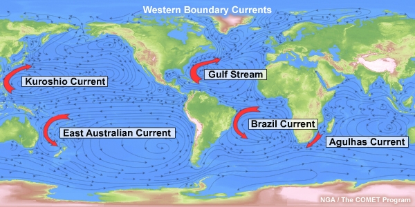
North Wall Events invariably involve western boundary currents. These are the currents that occur along the western margins of ocean basins and include the Gulf Stream, Kuroshio Current, and Agulhas Current. With regard to North Wall events, the most significant aspects of western boundary currents are their warm SSTs and their high velocities.
Introduction
-
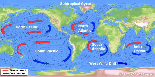
Western boundary currents comprise one portion of larger circulation patterns referred to as subtropical gyres. There are five subtropical gyres in the world’s ocean basins. These include gyres in the north and south Pacific, north and south Atlantic, and Indian Oceans. Each gyre comprises a westward-flowing equatorial current, poleward-flowing western boundary current, eastward-flowing midlatitude current, and an eastern boundary current that returns to the equatorial current. Note that in the southern hemisphere, the West Wind Drift, also known as the Antarctic Circumpolar Current, provides the eastward-flowing segment of the gyres.
Subtropical Gyres
-
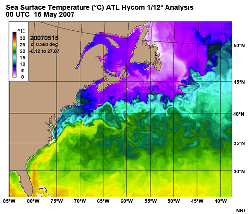
Western boundary currents probably constitute the most familiar ocean currents and for good reason. Because they originate at low latitudes, they bring warmth to higher latitudes. For example, this image shows sea surface temperatures in the northwest Atlantic Ocean. You can clearly see a tongue of warmer water moving up the U.S. eastern seaboard and then eastward across the North Atlantic. Heat from the Gulf Stream keeps northern Europe habitable.
WBC SSTs
-
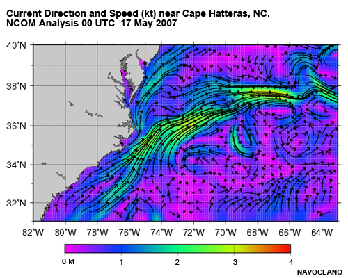
Western boundary currents are among the strongest currents. Velocities in western boundary currents frequently exceed 1 m/s (2 kt). For example, this plot shows a model forecast of current speed for the Virginia Capes region. It shows regions of 3 knots or more in the Gulf Stream east of Cape Hatteras.
WBC Current Speed
-
The high speed and large volume of western boundary currents results from a process known as western intensification. In response to the spin of the earth and friction along the coast, the centers of the subtropical gyres are displaced westward. In essence, water on the west side of a gyre must pass through a narrower, better-defined channel. Meanwhile, return flow on the east side of the gyre is less constrained and much more diffuse.
Besides the Gulf Stream, other notable western boundary currents include the Kuroshio Current off Japan, the Agulhas Current off southeast Africa, and the Brazil Current.
Western Intensification and WBCs
-
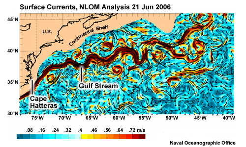
Global maps of ocean currents predictably fail to depict the details of the currents’ paths. The currents frequently bend and meander. This is particularly true of western boundary currents once they depart from the edge of the continental shelf. For example, this image shows the bends and meanders of the Gulf Stream northeast of Cape Hatteras along the U.S. East Coast.
Frequently, loops and meanders in the current close off to form isolated eddies that continue to spin. On the warm side of the current, eddies will have a cold core, while on the cold side of the current, eddies will have a warm core. These eddies can persist for a period of months to years and will continue to migrate along with the flow in which they are embedded.
Note that the warm core eddy spins clockwise while the cold core eddy spins counterclockwise.
For more information on ocean currents, see the COMET module Introduction to Ocean Currents.
Meanders and Eddies
-
Case Study: Gulf Stream January 2007 / Oceanography
Case Study: Kuroshio Current March 2006 / Oceanography
Case Examples
Stability in the Marine Boundary Layer
-
The high winds associated with typical cool season North Wall events arise from two factors:
1. A decrease in friction as the wind moves offshore and
2. Destabilization of the marine boundary layer (MBL) as cold air advects over warm water.
This section examines the MBL and how it changes in response to cold air advection.
-
The marine boundary layer differs substantially from the boundary layer over land. These differences have important forecast implications, particularly for wind and fog forecasts.
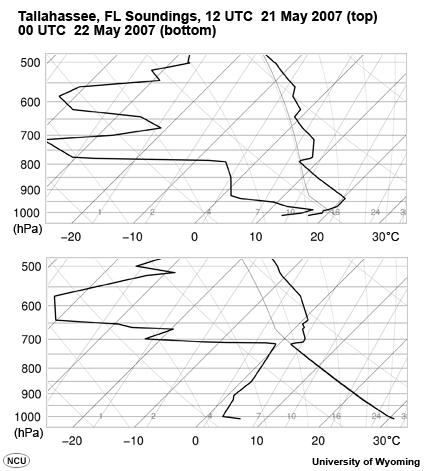
The lower atmosphere warms and cools through conduction from the surface. Land warms and cools substantially over the course of a day. As a result, we typically see a shallow surface-based inversion form at night, followed by a well-mixed boundary layer during the day. With strong heating, this mixed layer can extend 10,000 feet or more above the surface.
Here we see morning (12Z) and afternoon (00Z) soundings for Tallahassee, Florida. The morning sounding shows a surface-based inversion extending to about 925 hPa. The afternoon sounding shows a mixed layer extending to nearly 700 hPa.
In contrast to land, sea surface temperatures typically remain nearly constant over short periods of time. This results from several factors:
- the high thermal capacity of water,
- the ability of solar energy to penetrate many meters into the ocean, and
- water’s ability to mix readily.
As a result, we rarely see a surface-based nocturnal inversion over the ocean. Furthermore, with a long trajectory over water the surface air temperature approaches the water temperature.
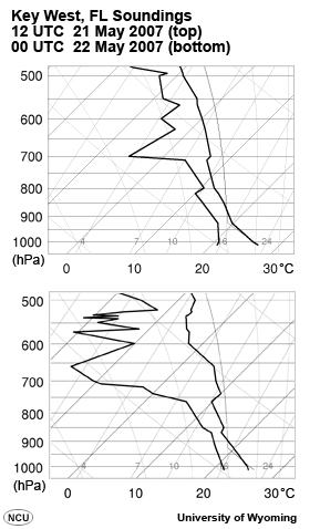
In addition, dry air moving over water rapidly moistens, which promotes low-level convective mixing. This results in a relatively moist boundary layer with a surface air temperature close to the sea surface temperature.
Here we see morning (12Z) and afternoon (00Z) soundings for Key West, Florida. Note the small changes to the temperature and dewpoint profiles over the course of the day. Lapse rates are conditionally unstable and dewpoints indicate relative humidity about 70%-80% throughout.
Introduction to the Marine Boundary Layer
-
Stability
Stability in the atmosphere refers to the degree to which air is prone to vertical motion. An unstable atmosphere is highly prone to vertical motion, while a stable atmosphere will resist vertical motion. An inversion, where temperature rises with increasing height, is a special case of a highly stable atmosphere.
If you are not familiar with atmospheric stability, a brief overview may be in order. Please review the following short topics on stability from the COMET module Skew-T Mastery:
The Parcel Method (https://www.meted.ucar.edu/mesoprim/skewt/navmenu.php?tab=3&page=2-1-1&type=flash)
Stability Types (https://www.meted.ucar.edu/mesoprim/skewt/navmenu.php?tab=3&page=2-2-0&type=flash)
Lapse Rates (https://www.meted.ucar.edu/mesoprim/skewt/navmenu.php?tab=3&page=2-3-0&type=flash)
-
MBL changes in Response to Cold Air Advection
When low-level air moves across horizontal gradients in the temperature of the earth's surface, the boundary layer stability changes. There are, of course, many caveats to this statement and this is not the only way to change boundary layer stability, but we will confine our discussion to this process.
In this module, we are going to focus on two particular cases:
- cooler air moving over warmer water (cold air advection or CAA) and
- warmer air moving over cooler water (warm air advection or WAA).
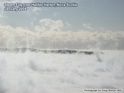
This photograph shows an extreme case of cold air advection over Halifax Harbor, Nova Scotia. Very cold, very dry air moves offshore from land to relatively warm water during an arctic outbreak. This results in steam fog formation over the water as the boundary layer rapidly warms and moistens.
-
Marine Boundary Layer Changes
This pair of temperature profiles shows how the marine boundary layer changes as very cold air flows over warm water during a cold air outbreak. The sounding on the left was taken on shore at Cape Hatteras, NC. The sounding on the right was taken offshore in the middle of the Gulf Stream about 100 km downstream of Cape Hatteras. Note that warming near the surface leads to a lapse rate in the lowest 100 m that exceeds the dry adiabatic lapse rate (i.e., superadiabatic) and is therefore absolutely unstable.
In general, cold air advection over relatively warm SSTs tends to cause moistening, mixing, destabilization, and deepening of the MBL. The rate and degree of mixing and destabilization depends primarily on the temperature difference between sea and air.
This plot shows how the LCL lowers and the MBL deepens as cold air advects offshore over the warm Gulf Stream.
-
Cloud Streets
Cold, shallow high pressure from an Arctic outbreak can be so cold that it can induce unstable lapse rates even over SSTs that are normally considered too cold to support convective mixing in the MBL. This regime can lead to local thermal circulations known as horizontal rolls accompanied by cloud streets forming parallel to the flow, as shown in this satellite image.
-
MBL changes in Response to Warm Air Advection
This animation shows how the temperature profile of a column of air changes as it advects over cooler water. We see near-surface air cool, which decreases the lapse rate and increases the stability of the boundary layer. With sufficient near-surface cooling, a low-level inversion forms and the boundary layer saturates, leading to fog formation.
In general, more stable conditions will exist in the MBL during warm air advection and unstable conditions will exist in the MBL during cold air advection.
-
Assessing MBL Stability - Sea/Air Temperature Difference
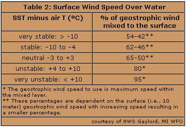
Forecasters assess low-level stability through a variety of ways. One obvious method is to examine the difference between sea surface and air temperatures. For example, the Gaylord, MI NWS forecast office has developed tables classifying the range of temperature differences. They use this information to forecast winds at the surface.
-
Assessing MBL Stability - Lapse Rate
Another way to assess MBL stability is to look at lapse rates. However, over the ocean we have few, if any, actual soundings to work with, which means that we must rely on output from NWP models to assess the lapse rate. The model's surface air temperature over water is often linked to a poor or coarse representation of the SST field. For this reason, the model surface air temperature can differ significantly from the true temperature. As a result, several NWS forecast offices modify the model's low-level temperature profile based on recent SST observations from buoys or satellites.
-
Seasonal changes
We can make some generalizations about seasonal changes to stability of the MBL by considering long-term tendencies. This chart shows monthly average sea surface and air temperatures at NOAA Buoy 41001, located 150 nautical miles east of Cape Hatteras, NC. Note that the largest temperature differences occur in the winter months. Also note that changes in sea surface temperature tend to lag changes in air temperature. For example, air temperatures tend to cool off sooner in the Fall and warm sooner in the Spring than sea surface temperature. Based on these mean temperatures, we can infer that the most stable MBL tends to occur from May through September, while the least stable tends to occur December through March.
-
MBL Depth
While the near-surface stability is helpful, it is also common practice to look at the temperature profile within the MBL to determine the depth of the instability (or stability), and hence the MBL top. The top of the MBL is defined as the lowest level where the lapse rate decreases. On a sounding, this transition can be sharp and unambiguous, as in the case of a very stable subsidence inversion above the MBL, or it can be subtle, as in a lapse rate increasing (i.e., becoming more stable) only slightly from the dry/moist lapse rate evident in the MBL. In the latter cases, the exact break point is somewhat subjective.
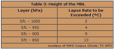
The forecasters at the NWS Corpus Christi, TX office examine lapse rates within several predefined layers over the marine area. If the lapse rate exceeds the threshold value for that layer, then that layer lies within the MBL and the top of the MBL lies at a still higher level. For example, if the lapse rate of the surface-900 hPa layer was 10°C but the lapse rate of the surface-850 hPa layer was 12°C, the height of the boundary layer would be roughly 900 hPa.
-
NWP Considerations
Many of the current (2006) high- and low-resolution models have a large number of layers in the BL. The current version of the NAM (WRF) model has 12 layers in the bottom 50 hPa. The GFS has 15 layers distributed across 1000-800 hPa with 7 of those between 1000-950 hPa (see GFS Vertical Coordinate System on COMET's Operational Models Matrix). Main errors in model BL profiles of wind, temperature, and dewpoint can be attributed to the turbulence and convective parameterizations, not the vertical resolution.
To determine which model is handling the MBL stratification well, use the buoy sites and compare wind observations with forecast model values. Also, compare the forecast pressure fields, on a synoptic scale, from the models to what actually occurs. If there is not a clear choice for the best initialized model, you will need to somehow blend the model solutions or develop your own.
Within regimes that produce rapid MBL changes, the forecaster should assess model forecast parameters at the finest temporal resolution available. For example, within a strong CAA regime over a relatively warm body of water, the MBL lapse rate can steepen quickly, and the depth of the MBL can increase rapidly, promoting more vigorous mixing and more rapid, efficient transport of momentum to the surface. In this case, an assessment of 1 to 3 hour forecast parameters might reveal the potential for an earlier onset of stronger surface winds, whereas an assessment of 12-hourly forecast data might miss this critical initial MBL growth stage and lead the forecaster to incorrectly forecast a later onset of stronger winds.
-
Case Examples
Case Study: Gulf Stream January 2007 / MBL Stability
Case Study: Kuroshio Current March 2006 / MBL Stability
Winds in the Marine Boundary Layer
-
Once we have determined the stability of the MBL, we can assess and predict the strength of the wind at the surface. Understanding the factors that determine the wind strength allows us to more accurately evaluate NWP model predictions. This section specifically addresses winds in the MBL and includes a methodology for forecasting them.
-
Atmospheric stability in the marine boundary layer (MBL) strongly impacts winds at the surface, and hence waves. In general, as instability increases in the MBL, winds tend to mix from above to the surface. Since winds aloft tend to be stronger, this usually results in stronger winds at the surface and, subsequently, larger waves.
Introduction
-
Friction Over Land vs. Water
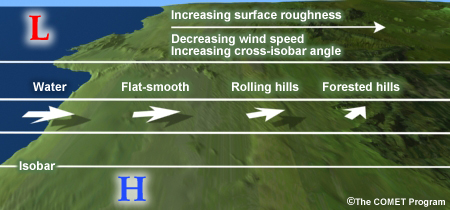
Over land, friction at the surface has a large impact on the near-surface wind. Vegetation and topography add a frictional force on the wind countering the pressure gradient and Coriolis forces. This shifts the wind away from geostrophic flow creating cross-contour flow toward lower pressure.
Over open water, the frictional force acting on the near-surface wind is generally much lower than over land. The water surface roughness is small compared to most ground cover. With less friction, winds at the surface are stronger, more consistent, and more nearly geostrophic in both speed and direction given a situation with the same atmospheric conditions as over a typical land mass.
The effects of the frictional force diminish with height until the wind is in a non-frictional dynamic state. This is typically characterized as gradient or geostrophic flow, which can then be further modified by dynamic features. This height, which varies with wind speed, lapse rate, terrain, and vegetation, is generally considered the top of the boundary layer.
-
Turbulence
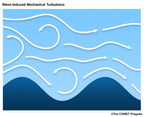
The interaction of the wind with sea surface waves results in mechanical turbulence. The resulting eddies formed by the rising and falling sea surface can extend vertically for tens of meters. The extent of these eddies is based on the height of the waves and the vertical wind shear near the surface.
In addition to mechanical turbulence, convective turbulence can be present due to rising plumes of warm air and compensating downdrafts. Convective turbulence can range from 100 to more than 1000 m in height, impacting wind flow in the turbulent layer. Stability is the primary factor in determining the depth of the MBL due to convective turbulence.
-
Stability and Friction
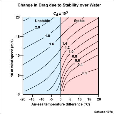
Friction at the sea surface (i.e., the drag coefficient) depends on both wind speed and stability. This plot shows contours of the drag coefficient for different values of wind speed and stability (as measured by the air-sea temperature difference at the surface). In general, drag increases with increasing wind speed and greater instability. Note the sharp increase in the drag coefficient as the air temperature falls below the sea surface temperature.
-
MBL Wind Profile
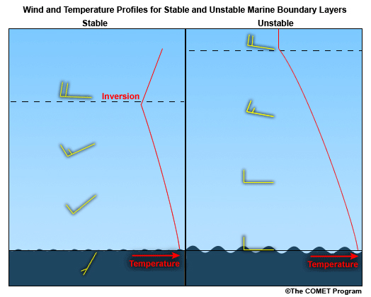
For a stratified (i.e., stable) MBL, one expects to see wind speed steadily increasing with height, but the upper boundary layer winds may have a point where they appear to be decoupled from the lower boundary layer. In other words, a point in the profile will show a relatively sharp change in wind speed and/or direction, and this point denotes the top of the boundary layer.
For a nonstratified (i.e., unstable) MBL, there will be less of a difference between the surface and upper boundary layer winds. Turbulent mixing of the unstable MBL allows the wind profile to become more uniform over time.
-
Using Stability and Geostrophic Wind to Estimate Surface Wind
Though current models have adequate vertical resolution to define the MBL, turbulence parameterizations can lead to errors regarding the vertical diffusion of momentum (i.e., wind) through low levels to the surface. Hence even a well-initialized model may have errors in surface winds.
In order to determine the percentage of the geostrophic wind speed at the top of the MBL that will mix to the surface, a forecaster needs to assess the low-level stability through the forecast period. The geostrophic wind speed can be obtained from model output or calculated based on an analysis of upper-air geopotential heights. The basic steps to estimating the surface wind speed over the ocean surface are:
- Assess the low-level stability to determine what fraction of the winds at the top of the boundary layer will mix to the surface.
- Determine the depth of the MBL.
- Determine the geostrophic wind at the top of the MBL.
- Using the stability analysis and the wind at the top of the MBL, determine the wind at the surface.
-
Assessing Low-Level Stability
Surface Wind Speed Over Water SST minus air T (°F) % of geostrophic wind
mixed to the surface< -7 55 -7 to 0 60 1 to 4 65 5 to 10 70 11 to 15 75 16 to 20 80 > 20 90 courtesy of NWS Charleston, SC WFO
There are a variety of ways forecasters assess low-level stability. One obvious method is to examine the difference between sea surface and air temperatures. For example, the Charleston, SC forecast office has developed a table classifying the range of differences and the respective percentage of the maximum MBL wind speed expected to be mixed to the surface.
An NWP model's surface air temperature over water is often linked to a poor or coarse representation of the SST field. For this reason, the model surface air temperature can be in error and lead to a false result if used in this table to determine stability (e.g., due to sparse observations over the marine area). An adjustment to the model profile near the surface may be warranted based on recent SST observations such as from a buoy or coastal station. As this table shows, the more unstable the situation, the greater the percentage of the geostrophic wind at the top of the boundary layer is mixed to the surface.
-
Determining the Depth of the MBL
Look at the temperature profile within the MBL to determine the depth of the instability (or stability), and hence the MBL top. If low-level conditions in the model output are not consistent with observations of air and sea surface temperatures, you may need to modify the model's low-level temperature profile to reflect those observations.
It’s important to remember that if advecting air crosses an ocean front between warmer and colder water, then the MBL will respond accordingly. In the case of CAA, the boundary layer will destabilize and deepen, especially as it moves over a region of warmer water. Tokinaga et al. (2006) showed that the boundary layer height tends to increase by 1 km as the sea-air temperature difference increases by 7°C.
-
Determine the Wind at the Surface
Once the forecaster determines the depth of the MBL, it is a relatively simple task to find the model layer closest to the top of the MBL. Depending on the model and the available data, this may be a pressure height (for example the 950 hPa level) or it may be a sigma level (for example 0.99 sigma).
Given the appropriate geostrophic wind and stability assessment, it should be fairly straightforward to forecast wind at the surface. Using the table developed at the Charleston, SC NWS Forecast office, one simply applies a percentage to the geostrophic wind based on the air-sea temperature difference. Your forecast office may have slightly different ways to assess stability or determine the appropriate geostrophic wind, but they will likely follow some variation on this methodology.
-
NWP Considerations
To determine which model is handling the MBL stratification best, use the buoy sites and compare wind observations with forecast model values. Also, compare the forecast pressure fields, on a synoptic scale, from the models to what actually occurs. If there is not a clear choice for the best initialized model, you will need to somehow blend the model solutions or develop your own, based on experience.
Within regimes that produce rapid MBL changes, the forecaster should assess model forecast parameters at the finest temporal resolution available. For example, within a strong CAA regime over a relatively warm body of water, the MBL lapse rate can steepen quickly, and the depth of the MBL can increase rapidly, promoting more vigorous mixing and more rapid, efficient transport of momentum to the surface. In this case, an assessment of 1 to 3 hour forecast parameters might reveal the potential for an earlier onset of stronger surface winds, whereas an assessment of 12-hourly forecast data might miss this critical initial MBL growth stage and lead the forecaster to incorrectly forecast a later onset of stronger winds.
-
Wave Forecasting Implications
If model stratification is poorly representative of actual conditions, then model winds and waves may be over-forecast for a stable MBL or under-forecast for an unstable MBL.
Frequently there is an over forecasting of wave height by the wave model in stable MBL conditions where one would observe fog or stratus via satellite observations. Generally, wave heights are under-forecast by the model in unstable MBL conditions such as during cold air outbreaks off the U.S. East Coast, explosively deepening systems, or tropical cyclones.
-
Case Examples
Case Study: Gulf Stream January 2007 / MBL Winds
Case Study: Kuroshio Current March 2006 / MBL Winds
Wave Growth
-
The rapid growth of waves in North Wall events results from strong winds at the surface. However, fetch and duration are also required. This section reviews the factors involved in wave building and demonstrates a forecast method.
-
Factors
Three basic factors contribute to wave growth:
- Wind speed
- Fetch or fetch length
- Wind duration
Fetch is the distance over water which the wind blows from a constant direction and at a constant speed. Duration is how long the wind affects that distance.
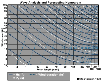
This Wave Analysis and Forecasting Nomogram quantitatively illustrates the relationship between wind speed, wind duration, fetch length, and wave growth. Wind speed is charted on the y-axis and fetch length on the x-axis. Contour lines represent wind duration, wave height and wave period. We will discuss these relationships and this nomogram as we proceed through this section.
The material is this section was derived from a more complete treatment in the COMET module Wave Life Cycle I: Generation
-
Wind Speed
As we see in the wave nomogram, wave height generally increases with increasing fetch length for a given wind speed. However, this only occurs to a point. Note in the nomogram that the wave height contours (dark blue) flatten out toward the right side. As wave height increases, wave speed also increases. When the wave speed equals the wind speed, the waves stop growing. In deep water, the wave speed (in knots) equals 3 times the wave period (in seconds). Thus waves with a period of 10 seconds have a wave speed of 30 knots, and will not grow larger if the wind speed is 30 knots or less.
-
Fetch Length
As we see in the wave nomogram, wave height generally increases with increasing fetch length. Note that wave growth occurs most rapidly in the first 100-200 n mi or so. Then just as with wind speed, waves eventually stop growing given a long enough fetch. For example, given a wind speed of 12 kt, waves grow until the significant wave height approaches 4 ft at a fetch of about 500 n mi. Waves then stop growing larger, regardless of any additional fetch.
-
Fetch Width: Impact of Fetch Dimension
A fetch is like a snowflake in that no two are alike. Some fetches are long and narrow while others are short and wide. The dimensions of the fetch have an impact on wave growth by determining the amount of wave energy that stays within the wave generation area. Within the fetch a general wind direction can be determined, but many small variations will occur. This means that there are smaller waves created that propagate out of the sides of the fetch region while the predominant wind direction generates larger waves that exit from the downwind end of the fetch.
Note that the winds exiting the side of the fetch would have a greater distance within which to grow if the fetch width increased.
-
Fetch Width: Wave-Wave Energy Transfer
Within the fetch there is a wave-to-wave energy transfer. This is what helps build the larger waves. Wave energy also bleeds out the sides of the fetch due to wave spreading. Compare fetches of different widths. Fetch B covers three times the area of Fetch A. While the same amount of energy is dissipated from the sides of both fetches, the amount lost as a percentage of the fetch's total energy is larger in fetch A. Therefore a narrower fetch will result in smaller waves.
-
Wind Duration: Definition
We have seen how wind speed and fetch affect wave growth. Now we will investigate the third wave growth factor: wind duration. Duration is the length of time a wind in a given fetch affects wave growth. Given a high wind speed and long fetch length, the longer the wind blows, the larger the waves will grow.
-
Wind Duration Limitations
Even with sufficient wind speed and fetch length the duration can be the limiting factor in wave growth. This can occur with fast-moving storms where the area of strong prefrontal winds is aligned with the angle to the general storm direction. In this case the fetch is constantly affecting a different part of the water surface for a short period of time.
Mesoscale events are usually of short duration. These can include thunderstorm outflow boundaries, sea breezes, and land breezes. Strong, long-lived wind events can have a fetch persist for days, but if the fetch is moving perpendicular to the storm direction, the duration over any given area of water will be short. This can occur on the leading and trailing sides of hurricanes or around deep synoptic-scale lows.
-
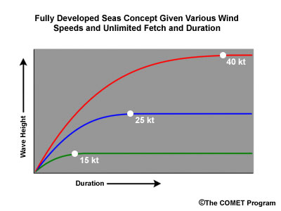
Fully Developed Seas: Definition
A fully developed or fully arisen sea describes a sea state in which the wave's characteristics are not changing. Provided the wave growth is not limited by fetch length or duration, wave growth eventually reaches equilibrium where the energy given to the waves by the wind equals the energy dissipated by the waves through dispersion and breaking.
-
Fully Developed Sea Limitations
Ultimately wave growth is determined by the wind speed. The wave height is generally limited by the fetch length and wind duration for strong wind speeds. It is difficult for a fully developed sea to occur with wind speeds of 40 kt or greater because the fetch length and duration needed to create unchanging waves is relatively large. Even winds at 25 kt will need a moderate amount of time to become fully developed. It is much more likely for winds of 15 kt or less to produce fully developed seas since a much shorter fetch length and duration are needed. The stronger winds that affect many of the oceans and large lakes will not be able to reach their potential in terms of wave height generation due to changing or limiting fetch length and duration.
-
Case Examples
Case Study: Gulf Stream January 2007 / Wave Forecast
Case Study: Kuroshio Current March 2006 / Wave Forecast
Wave-Current Interactions
-
Introduction
In North Wall events that result from cold air outbreaks, the wind is typically blowing offshore over a warm current flowing parallel to the coast. The resulting waves are moving in a direction nearly perpendicular to the current. Consequently, there is little interaction between these waves and the current. However, there are other circumstances under which wind, waves, and currents interact to build higher, steeper seas. That is the focus of this section.
-
Wave Growth due to Increased Wind Stress
The most important aspect of wave growth is the relative speed of the air above the water surface. This governs the amount of kinetic energy transferred from the wind to the water. In the presence of a current, the relative speed of the air just above the surface depends on whether the current is moving in the direction of or opposing the wind. When the wind and the current move in the same direction, the relative speed of the air moving across the ocean surface is less than if the ocean were not moving. This reduces the effective energy transfer and potential wave growth. When the wind is blowing opposite to the ocean current the relative speed of the air is increased, thereby increasing the energy transfer and potential wave growth.
-
Effect of Currents on Swell
When swell that originates elsewhere encounters a current, its wavelength and height change. As this animation shows, when the current is flowing in the same direction as the waves, the wavelength increases while the wave height decreases. This situation might occur when, for example, southerly swell from a tropical storm in the Caribbean encounters the Gulf Stream along the eastern United States.
Where currents oppose waves, as shown here, wavelengths decrease and heights increase. This situation might occur when swell from a winter storm in the North Atlantic encounters the Gulf Stream. If the waves are steep enough and the current strong enough, waves will break.
-
How big do waves get?
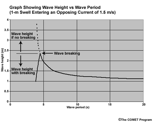
The relative importance of the current on the wave height is not a simple relationship and depends upon the initial steepness of the wave and the speed of the current it is entering. The steepness depends on the wave height and wavelength. The wavelength, in turn, depends on the wave period. This chart shows the resulting wave height when a 1-m swell encounters an opposing current of 1.5 meters per second (about 3 knots - equivalent to the speed of the Gulf Stream). It is based on linear wave theory as described by Baschek (2005). We use the wave period across the bottom axis instead of the wavelength because the wave period is typically available in observations and model data. As the wave period decreases, the wavelength shortens, resulting in steeper waves.
To apply this chart, one would find the appropriate wave period outside of the current, then trace vertically up to the dark line. From there, read the resulting wave height on the left. Thus a 1-m swell with a 10-second period, would increase to about 1.3 meters when it enters an opposing current of 1.5 meters per second. Similarly, a 1-meter swell with a 5-second period would nearly double in height.
At a period of just over 4 seconds, the wave is so steep that it starts to break, and its height rapidly diminishes. This chart is based on a breaking criteria where the wave breaks when the ratio of the amplitude to the wavelength falls below 1:7. Somewhere near 4 seconds, the wave speed falls below one quarter of the current speed and the wave is stopped dead. It breaks completely and its height falls to zero.
To determine wave heights for more general cases, we have created a wave-current interaction calculator.
-
Refraction of Waves
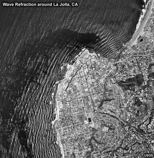
You may recall that ocean waves refract when they encounter shallow water near shore. The result is that waves bend around points and into bays so that they align themselves with the coastline. This aerial photograph shows wave refraction around Point La Jolla in Southern California. Wave refraction occurs because the waves slow as they "touch bottom" near shore. This allows waves in deeper water to "catch up". The result is that waves bend to an orientation more parallel to the shoreline.
Because waves slow when they encounter an opposing current, they also refract. As a result, wave crests become more parallel to the current direction. As waves encounter progressively faster current, they refract more.
Also recall that points and other coastal headlands concentrate wave energy, while bays and inlets diffuse wave energy. Just as bends in the coastline concentrate or diffuse wave energy, bends and meanders in ocean currents similarly concentrate and diffuse wave energy.
Several studies support this conclusion. This figure shows an example from a study of wave refraction in the Gulf Stream by Wang et al. (1994). We can see that a meander in the current acts like a lens, changing the swell direction and wavelength and focusing a great deal of wave energy at a single point, resulting in larger waves near that location.
In another study of wave-current interaction in the Gulf Stream, McCulloch (2006) found that when the waves propagated against the 2 m/s currents in the Gulf Stream there was a 1 meter (20%) increase in wave height and a 2 second increase in wave period. Within anticyclonic eddies the wave steepness increased by 30% and in cyclonic eddies it decreased by 30%.
Holthuijsen and Tolman (1991) found that the dominant wave-current effects were the trapping of locally generated storm waves in the straight Gulf Stream when the wind was against the current, and the reflection of waves back to the open ocean if they approached the Gulf Stream from a current-following direction. They also investigated an idealized Gulf Stream ring and found that the currents can cause large variations in the wave height and period, because rings contain both counter currents and following currents with respect to the waves. Counter currents enhanced wave height by 30%. Following currents reduced wave heights by 30%.
-
Rogue Waves
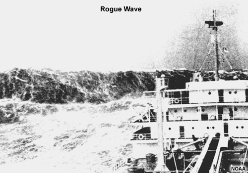
Wave refraction is one possible origin for rogue waves (traditionally defined as waves taller than two times the significant wave height). In fact, most ship encounters with rogue waves occur near strong western boundary currents like the Gulf Stream, Kuroshio Current, or Agulhas Current. The circumstances typically entail large waves moving against the current.
-
Case Examples
Case Study: Tropical Cyclone Florence September 2006