Introduction

This module is in three sections:

• post-processing/Products,
• Statistical Guidance, and
• Assessment Tools.

Specific topics covered include the impact of post-processing and how to account for it, the statistical methods used to enhance raw model output including how statistical guidance products like MOS are generated, as well as NWP verification methodologies and use of daily model diagnostics.

Post-Processing

* Post-Processing Overview

Models do not explicitly predict certain information, such as the height of the freezing level, the precipitation type, or boundary-layer winds. Yet this information is available to forecasters as part of the model output. If the models do not predict these fields directly, how and when are they generated? It's done through post-processing - the process of transforming raw model data into a format that's useful to forecasters.

By going through this section, you'll better understand:

• Why model post-processing is needed
• What's typically done during post-processing
• How the postprocessor interacts with the forecast model
• Whether it's always better, or even advisable, to view model data on the native representation of the model
• Why diagnostic or derived parameters are needed
• How derived fields are typically created

Need for Post-Processing

Why do we need post-processing?

Numerical models often produce output that's either not usable by forecasters or that's lacking in useful products. Model output on sigma, hybrid sigma-theta, or hybrid sigma-pressure layers is nearly meaningless to forecasters. Post-processing translates model output from the model's native forecast grid, vertical coordinate, and variables into meaningful, standardized output. It produces common forecast parameters at standard vertical levels as well as supplemental products and fields.

Post-Processing Process

What's typically accomplished during post-processing?

During post-processing

• Forecast fields are converted from the native representation of the model computational structures to meteorologically meaningful coordinate systems. This can involve both
  • Transformation from spectral coefficients to grid points (or specific locations)
  • Horizontal and vertical interpolation of native model grids to World Meteorological Organization standard "display" grids (or specific locations) and a specified variety of vertical levels (isobaric levels, possibly some isentropic, sometimes at "tropopause", etc.)
• Standard output variables as well as derived and special field variables are computed from model forecast data. These additional variables typically include
  • Common fields, such as mean sea-level pressure, relative humidity, dewpoint, and geopotential height
  • Vertically integrated parameters such as CAPE, CIN, PW, and stability indices
  • Tropopause-level data
  • Flight-level fields
  • Freezing-level information
  • Boundary-layer fields

Additional post-processing may occur locally at the field office. For example, AWIPS generates a wide variety of additional derived parameters from the postprocessed model data.

Interpolating from Native to Post-Processed Grids

Is it always better, or even advisable, to view model data on the native representation of the model?

All forecast computations within a model are carried out on its native representation, which can be either

• The grid type and vertical coordinate of a grid point model (such as the Arakawa B grid and hybrid sigma-pressure coordinate of the WRF-NMM Model)
• Within the wave representation (and grids) and vertical coordinate of a spectral model

In either case, the native representations of forecast data are usually not in a format that forecasters can directly use. For example, spectral data are represented as individual wave positions with varying amplitudes and rotational and non-rotational wind components, which may be difficult to interpret.

Model data must be translated to a meteorologically useful format both horizontally and in the vertical. The process by which this is accomplished is illustrated in the graphic.

Click the Step boxes (Step 1, Step 2, and Step 3) for more information on each step.

Step 1: Point Data Conversion

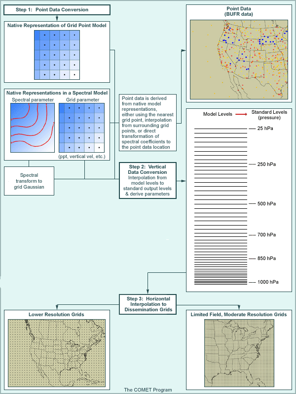
For spectral models, the postprocessor transforms the spectral coefficients to the uniform Gaussian or physics grid in the same way that the forecast model does. (Recall that a spectral transformation is carried out at each time step so physics and non-linear dynamics can be computed on a grid.)

Point data (BUFR data) are derived from the native representation of the model. For grid-point data, point data are created using the nearest grid point or through an interpolation process. For spectral models, spectral coefficients are expanded directly at the interpolation location on the native vertical coordinate. Note that in either case, point datasets preserve the models' native vertical resolution.

back to image

Step 2: Vertical Data Conversion

The native model output is then interpolated from native model levels to standard output levels (typically pressure). It is important to note that

• The computation of most special fields/parameters is carried out on the model's native vertical coordinate (before the data are interpolated in the vertical from model levels to standard vertical levels)
• Some supplemental fields, such as vertically integrated parameters, may be computed during the vertical interpolation to common levels

back to image

Step 3: Conversion to Dissemination Grids

Typically, the vertically interpolated grids are very large, which makes them difficult to disseminate operationally. Because of this and issues of delivery timeliness, these grids are converted (interpolated again) to dissemination grids. These may be lower-resolution grids with a full suite of parameters, or high-resolution grids with a limited number of parameters and levels, such as surface or other specialty grids.

It is important to emphasize that the dissemination model data viewed by forecasters have been interpolated at least twice, which again includes some small degree of smoothing beyond any smoothing done during the forecast processing. Dissemination grid resolutions with less than a 2:1 difference in size contain almost all of the information present in the native representation of the model.

back to image

Need for Diagnostic and Derived Parameters

Why are diagnostic or derived parameters needed?

Basic model output typically includes prognostically produced parameters, such as

• Pressure
• Temperature
• Specific humidity
• Component winds
• Diagnostically produced products computed from the basic forecast fields during integration

Aside from these standard fields, many other parameters make useful forecast tools but are not yet available as basic model output. Post-processing serves another useful function by deriving these products from the primary model fields. As was mentioned earlier, these derived and supplemental fields are computed on the model's native vertical coordinate and perhaps even its native horizontal (spectral or grid point) representation.

* Derivation Techniques & Fields

What is "typically" involved in creating derived fields?

There are many derivation techniques for parameters ranging from mean sea-level pressure to convective available potential energy (CAPE). Many of the commonly derived parameters are calculated using general formulae and are not tuned to any specific model. These fields are typically computed at each grid point from vertically interpolated base fields and then placed on the post-processed grids.

Common derived fields include:

• Temperature - from virtual temperature
• Sea-level pressure - from integrated virtual temperature and surface elevation/pressure
• Geopotential height - from integrated virtual temperature
• Dewpoint temperature - from specific humidity
• Relative humidity - from specific humidity
• Absolute vorticity - from winds
• Precipitation type - from vertical temperature and dewpoint structure, using precipitation type algorithms, or from actual forecast precipitation reaching the ground (e.g. WRF-NMM using Ferrier precipitation scheme)
• Tropopause-level data (pressure, temperature, horizontal winds, and vertical wind-shear)
• Cloud and other RH products
• Flight level/aviation fields (temperatures and winds)
• Freezing-level data (freezing-level heights and RH)
• Hazards products (surface visibility, icing, turbulence, wind chill, and heat index)
• Sounding/severe weather fields (K index, Storm Relative Helicity, LI, CAPE, and CIN)
• Surface-based fields
• Low-level fields (10 m and 2 m - not the same thing as the surface fields)
• Boundary-layer fields

Note that these fields may be model-specific and are addressed in the Operational Models Encyclopedia.

Beyond Interpolation to Post-Processed Grids

Deterministic NWP

Raw NWP model data is further processed beyond mere interpolation to pressure levels or to nearest neighbor points, to deal with model deficiencies of various kinds. These include, but are not necessarily limited to

• Bias correction (typically based on recent model performance history)
• Downscaling (typically based on data sets such as MOS developed from high resolution surface data and high resolution topography)
• AWIPS internal processing functions that produce additional parameters

Specifics on bias correction and downscaling will be discussed in upcoming NWP Course webcasts in Unit 2. Links to specifics on AWIPS parameters can be found in the Operational Models Encyclopedia linked from the NWP model matrix.

Probabilistic NWP: Ensemble Forecast System Post-Processing

Ensemble forecast systems (EFS) require considerable post-processing to distill the huge amounts of data contained in them. Post–processed data include computation of statistics for the ensemble membership, including but not limited to:

• Ensemble mean and standard deviation
• Percentile values
• Probability of exceeding threshold values

These data can also be bias corrected and downscaled, just as the deterministic NWP model data can. Further general discussion of ensemble products can be found in the section on ensemble products in Ensemble Forecasting Explained, with products for specific EFS found in the Operational Models Encyclopedia.

Summary Question

Summary

As an operational user of numerical model output, here are the key points about post-processing to keep in mind:

• post-processing transforms raw model data into a format that's useful to forecasters (in terms of size, timeliness, and range of products). It produces common forecast parameters at standard vertical levels as well as supplemental products and fields. It may do this, though, at the expense of representing model fields precisely
• It's not practical or even advisable to view native model output on an operational basis since it may not be represented in a meteorologically useful format and may also lack useful fields and parameters
• Having access to the highest resolution dissemination grids is usually very beneficial
• Output at less than full model resolution does not necessarily imply any loss of information
  • Dissemination grid resolutions with less than a 2:1 difference in size contain almost all of the information present in the native representation of the model
• Output at less than full model resolution is much more practical for dissemination

Statistical Guidance

Introduction

Statistical guidance (SG) based on NWP output is simply the application of formal statistical analysis to both raw model output and observed weather variables, with the intent of improving upon the numerical model forecasts.

Statistical methods have traditionally been an important and useful tool in forecasting. Application of these methods to model guidance and observed weather conditions represents one of the more important operational tools available to forecasters today. However, as with any tool, the more you understand statistical guidance by knowing both how it is constructed as well as what its strengths and limitations are, the more effectively you will be able to use it and the better your results will be.

Note that while the rest of this section will focus on MOS and Perfect Prog techniques, SG also includes post-processing of ensemble forecast system data using statistical techniques, and bias correction of both deterministic and ensemble model data (information forthcoming in a future module). Additionally, SG is provided through a gridded MOS product – MOS developed using same regression principles explained here but produced on grid instead of at stations. Information and training on Gridded MOS are available.

This section will provide you with the information to understand when SG will perform well and not-so-well. You'll also learn to identify situations when SG can be a useful tool and when it may be leading you down the garden path.

Why Do We Need SG? (Aren't the Models Good Enough?)

While numerical weather prediction has undergone significant improvements over the last decade, it is still not perfect. Model forecasts are subject to systematic errors that inhibit their performance. In addition, models may be lacking fields and products useful to the forecaster. Finally, because model output is deterministic rather than probabilistic, it does not express the uncertainty involved in different forecast situations.

Application of SG can provide the following advantages over direct model output:

• A means of removing certain systematic errors in model guidance at specific locations as well as accounting for degraded accuracy with increasing forecast projection
• Forecasts of variables that cannot be directly derived from the forecast model output
• A measure of confidence that specific weather events will occur (i.e., probability)

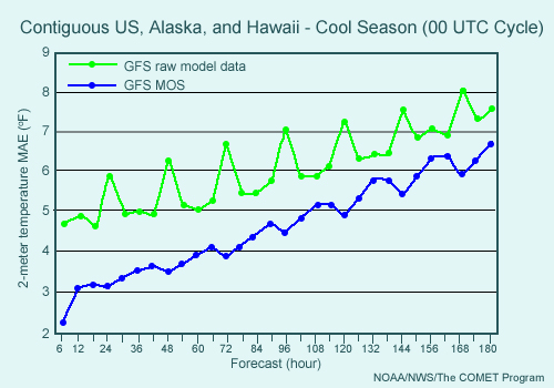
In the above example the mean absolute errors (MAE) generated from raw and SG data (GFS and GFS MOS respectively) output are shown. Notice that the MAEs generated from the SG data are significantly smaller than those of the raw forecasts at all projections. Statistical forecasts generated from NWP output can compensate for some systematic errors, improving the quality of the forecast.

Regardless of its strengths, statistical post-processing of model output is still limited by the data put into it (the M in MOS doesn't stand for miracle). Some fundamentally important points about SG are:

• SG can make a good NWP forecast better, but cannot fix a bad NWP forecast.
• It is designed to fit most cases, assuming a normal distribution, therefore in skewed climate regimes or outlier cases, SG won't work as well.

In this section, forecasters will learn to make better use of SG through a better understanding of

• The two approaches used to produce SG
• Statistical techniques used in conjunction with NWP output
• The developmental techniques used in implementing SG
• Operational issues and trends in SG

Statistical Guidance Approaches

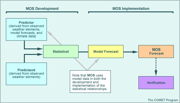
There are two SG approaches that are most commonly applied to NWP output for use as operational guidance, perfect prog (PP) and model output statistics (MOS). On a basic level, both approaches are analogous to what an experienced forecaster does in practice. An operational forecaster defines relationships between observations and forecast data throughout his or her career (including accounting for model biases), and then applies these to the interpretation of operational numerical model output, improving upon the raw model forecast (hopefully). An example of this is the operational practice of defining a correlation between observed 850-hPa temperature and maximum temperature under clear conditions, and then applying it to model forecasts of 850- hPa temperature to aid in forecasting the high for the day. But while the forecaster carries this enhancement out subjectively, SG accomplishes it through objective means.

Important Terms

• Predictand: The dependent variable that is to be forecast by the SG. Predictands are derived from observed weather elements. Examples of SG predictands include temperature, precipitation probability, visibility, etc.
• Predictor(s): The independent variable (or variables) used in conjunction with the predictand to derive a statistical relationship that drives statistical guidance. Three basic types of predictors are used: model output, observed weather elements, and climatological data.
• Probability: A quantitative expression of uncertainty.
• Persistence: Also referred to as the classical method, it is the statistical dependence of a variable on its own past values (based solely on observed weather elements). Persistence can account for time lag by relating current predictor data to future predictand data as part of the development of the statistical relationship. For example, what is currently occurring in an observed weather element (i.e., temperature) is related statistically to the precipitation type that will occur at some future forecast time.
• Climatology of the Sample: Relative frequency of a number of weather events within the developmental dataset (can be thought of as the mean of the predictand data).

While both MOS and the perfect prog utilize similar statistical methods and mathematical procedures that are borrowed from other disciplines, there are significant differences in the approaches they take. These approaches are discussed in the next few pages.

* Perfect Prog

The perfect prog (PP) statistical technique develops equations based on the relationship of co-existing observed weather elements (including climate data), which are then applied to raw model output to produce statistical guidance. PP equations may or may not account for time lag in their development (unlike persistence methods which must account for a lag time); instead they may relate simultaneous predictors and predictands (i.e., values from the same time frame) or they might relate a predictand to a predictor observed several hours earlier. While both the classical and perfect prog approaches relate the predictand to observations, the classical approach must have a time lag in the development of its equations. The perfect prog approach may or may not incorporate a time lag in the development of the relationships, depending on both the predictand and the available predictors.

Time lag within the PP approach is accounted for by applying the derived relationships to forecasts from the numerical model. For example, with the use of 1000-500 hPa thickness to differentiate between rain and snow, PP develops relationship equations from observations of the thickness (predictor) and observed precipitation type (predictand). These relationship equations are then applied to model forecasts of the predictor (thickness) to produce a forecast of precipitation type.

Advantages

• PP does not require a developmental dataset of historical model data.
• PP guidance is likely to improve with improvements to the raw model forecasts.
• Multiple predictors can be used, resulting in a better fit to the predictand data and, possibly, more accurate guidance.

Limitations

• Because historical model data are not used in the development of the statistical equations, systematic model errors cannot be accounted for in PP forecasts.
• May also affect the reliability of PP guidance at longer projections (PP cannot account for the deterioration of model forecasts with lead-time).
• Inaccurate or unreliable model forecasts of particular parameters (such as 2-m temperatures) may preclude their use as predictors.

Model Output Statistics (MOS)

The MOS technique develops relationship equations from both observed and model forecast weather elements, which are then applied to raw model output (the same or similar model) to produce statistical guidance. MOS is used frequently in the National Weather Service. Because MOS uses NWP output in both the development and implementation of the statistical equations, time lag can be incorporated into the relationships as well as an accounting of certain systematic model errors such as a dry bias.

For example, forecasters unconsciously apply the MOS technique subjectively when using model forecasts of 70% RH to estimate cloud forecasts. This practice may work in a number of cases but a problem arises when the model has a dry or wet bias and lower/higher model RH values are not used to estimate clouds. In the case of a dry bias, if the forecaster does not account for the lower model RH values by using model RH values of less than 70%, clouds are likely to be underforecast by the model and the forecaster. Even if the forecaster does make some adjustment by using 60 or 65% RH, the selection of these values is somewhat subjective and not necessarily based on an established relationship. However, if MOS guidance is used to estimate the clouds, the statistical relationships developed for that model will already take into account such systematic errors as the dry bias.

Advantages

• Because historical model data is used in development
  • MOS can account for systematic model errors and deteriorating model accuracy at greater forecast projections.
  • MOS can account for the predictability of model variables by selecting those that provide more useful forecast information. For example:
    • Using 850-hPa temperature forecasts as opposed to 2-m temperature forecasts to generate surface temperature guidance where the 850-hPa temperature is typically more accurately forecast
• Multiple predictors can be used, resulting in a better fit to the predictand data and generally more accurate guidance.

Limitations

• MOS requires a developmental dataset of historical model data that is used as the predictor.
  • This can be inefficient, particularly in situations where the operational model suite is evolving (requires redevelopment of statistical relationships).For example:
    • Improvements to model systematic errors will result in degraded MOS guidance until the developmental dataset is updated.

*Statistical Techniques

There are several statistical techniques that are used to develop the relationships defined in both the PP and MOS approaches to statistical post-processing of NWP output. The most common method is that of multiple linear regression, which is presented in detail in the following pages. Several other, equally viable, methods are also mentioned (although in less detail).

* Linear Regression

Linear regression determines the relationship between the predictand and predictor(s) that comes closest to fitting all the data in a dataset. More specifically, linear regression is a mathematical technique that derives the relationship (in the case of two variables the relationship is a line) between the predictand and the predictor in a way that minimizes the sum or average of the squared errors. This is illustrated in the graphic.

Shown graphically using a scatter plot of predictands (y) vs. predictors (x) is the line that best represents the relationship between the two variables such that it minimizes the residual error (in this case the total or average vertical distance between all points and the optimal line). This is typically accomplished using a least squares regression, which minimizes the sum of each of the squared errors (e) to fit the line to the data (the use of squared values eliminates sign issues).

* Multiple Linear Regression

Multiple linear regression is simply the application of linear regression using multiple predictors and only a single predictand. It is done in a series of steps known as forward stepwise selection.

The process can be thought of as being iterative, where predictors are selected such that the relationship between the predictand and each potential predictor is checked first using simple linear regression. The result is a list of predictors that are relevant to the predictand data. From the initial linear regression, an optimal or best predictor (i.e., one that has the best fit to the predictand data) is also determined. A second set of comparisons using forward stepwise selection is then carried out using the remaining list of relevant predictors. Each of these predictors is examined with respect to both the optimal predictor and the predictand, producing additional 3D relationships, rather than simply linear ones. Each subsequent predictor is selected on the basis of its contribution to the reduction of residual error when combined with the other variables already selected (both predictor and predictand). This process can continue as long as it makes sense (i.e., as long as the residual error is minimized) using as many additional predictors as is necessary.

Note that the group of predictands finally chosen through forward stepwise selection may not be optimal. Remember that the chosen predictors are the optimal grouping given their relationship with the best predictor that was selected first. It is possible then that a better statistical relationship can be defined using a group of predictors that does not include the single best predictor. The graphic below illustrates the process of multiple linear regression. Click boxes I and III for more clarification on those steps.

back to image

back to image

* Other Statistical Methods

There are several other techniques that may be used instead of multiple linear regression to generate statistical relationships between predictor and predictand. These include

• Kalman Filters
• Neural Networks
• Artificial Intelligence
• Fuzzy Logic

These methods still require samples of data on which to train the technique, and can potentially produce a very good fit to the dependent data (particularly highly non-linear datasets). However, this relationship may not prove to be a viable fit with respect to the independent data. In addition, these statistical techniques are much more difficult to implement than multiple linear regression. Ultimately many of these approaches do prove useful in addressing more difficult forecast problems such as visibility or QPF, but would be of little or no additional help in predicting pop, temperature, or wind.

Development Techniques

In addition to the statistical techniques used, choices of developmental techniques will also affect the nature of the SG products. These techniques may involve data selection, manipulation and grouping, as well as post-processing of SG output. Each of these development techniques has an impact on both the implementation and use of SG guidance. These are discussed in the following pages.

Data Grouping

The data used (both predictand and predictor) to derive the regression equations done in SG are often grouped to optimize the forecast relationships and improve the accuracy of SG guidance. This grouping is achieved using either of the following approaches:

Stratification of Data

• This technique involves decreasing the size of the developmental sample by separating data into subsets in order to improve the relationship between predictand and predictors.
• This is done according to a precise set of rules, typically according to season, model cycle, valid time (for the predictand), station or region, and weather element. The latter is accomplished by conditioning upon the occurrence of an event (such as using only precipitation cases to help develop algorithms for precipitation type forecast guidance), or map typing (stratifying data according to another relevant field or condition such as wind direction).

Pooling or Compositing of Data

• Pooling involves combining datasets in order to increase the size of the developmental sample. This is done to improve the likelihood of generating stable regression relationships, typically in cases where the predictand is a relatively rare event (such as the occurrence of precipitation or thunderstorms) so that a sufficient number of events are included in the dataset.
• When pooling data, it is assumed that the forecast relationships are not location or station specific. This assumption can be invalid, particularly in areas of strong orographic forcing (i.e., complex terrain), where the pooled sample may not be homogeneous. To compensate for the lack of homogeneity in a region, geoclimatic predictors like terrain height or event relative frequency (climatology) are used.

Regression equations can of course be developed using data at individual locations. Typically single site equations are used to predict weather elements that are highly dependent upon effects specific to individual locations or sites and occur commonly, such as orographic forcing due to complex terrain or significant surface discontinuities such as along a coastline.

Predictor Selection and Manipulation

Recall that predictor data may be of three types: model forecasts, observed weather elements, and geoclimatic data. Knowledge of the nature of the predictand and how it was selected and manipulated is important (what time period is covered, point or region, etc).

• In developing SG, it is important to use physically meaningful variables to relate predictand data to predictor data and to choose variables that can be reasonably forecast by the models. For example, model fields that are poorly forecast or unreliable, such as 2-meter temperatures, may not be as useful in predicting surface temperatures as other more reliable fields such as 850-hPa temperatures.
• Model data are often interpolated to a lower resolution grid before the data are used in the development of statistical relationships. This is done to simplify and minimize the amount of computations involved in the derivation of the SG equations (full model resolution model output is not always beneficial). However, this is done in addition to any interpolation carried out during the model's own post-processing and may be at the expense of representing model fields precisely (in cases of interpolating beyond 2Δ of the model's native resolution). Additional smoothing of model fields may be carried out before the development of the regression equations. Note: data from this lower resolution grid must also be interpolated to station locations for the development of regression equations. Therefore, statistical guidance for higher resolution models is not necessarily better than that for low resolution models.
• Model data at projections near (before or after) the observed time of a predictand may also be used as a predictor. Such data are treated in the same way that concurrent model data is, where the regression procedure determines the value of such data and weights it accordingly. An example of using model data at projections that are not concurrent with predictand times is in situations where there is a systematic phase error in the model data. In such cases the t-3 hour forecast might be better than the forecast that is concurrent.
• Geoclimatic data has impact as a predictor in two ways. Explicitly, the relative frequency of an event at a specific site is often used as a predictor, particularly in the application of data pooling. Implicitly geoclimatic data may carry more weight as predictor at the longer-range projections. The weighting depends solely on the regression analysis. For example, model data tends to lose value at longer lead times for some fields, thus the geoclimatic derived predictors will naturally carry more weight for that particular parameter (note that this does not necessarily mean that for all fields SG tends toward climate in the long range). However, because of the loss of skill in the model forecasts, SG tends toward the "climate" of the developmental sample.
• Current observations of various weather elements such as temperature, winds, sky condition, etc. may also be used as predictors although they are typically only applied in the shorter-range projections. Testing typically indicates the value added by observations for different projections; thus they might differ from element to element. For example wind observations may be used out to 15 hours, and temperature and dewpoint observations out to 36 hours. Beyond these projections, the use of observations adds little value beyond persistence.

Probabilistic Data

One of the strengths of SG output is that it provides probabilistic guidance, which expresses the uncertainty involved in different forecast situations. In SG, probabilistic forecasts are typically created using a binary predictand. Binary variables can have one of two values: one or zero (yes or no), which are determined using a threshold amount. For example a binary variable may be defined using a precipitation amount of 0.1 in. at a particular location over a three-hour period. Thus the predictand would carry a "yes" value for amounts exceeding the 0.1 in.

One method for generating probabilistic forecast guidance from binary variables is Regression Estimation of Event Probabilities (REEP). REEP simply applies multiple linear regression using a binary predictand, where the resulting predicted values generated from the forecast relationship are typically between 0 and 1. This can be thought of as a probabilistic forecast that the threshold used to determine the binary variable will be exceeded (for example, a .3 (30%) probability of exceeding 0.1 in. of precipitation).

We should note that since 2000, ensemble forecast systems have been coming more into use as a probabilistic forecast tool, additional to MOS products. So now there are two kinds of probabilistic information:

1. Probabilities derived from a single model, such as MOS does, and

2. Probabilities derived from forecasts of many model runs, such as ensemble forecast systems.

Ensemble probabilities will continue to play a more prominent role, as the data from them becomes more available to operational forecasters. One of the advantages of ensemble probability forecasts is that they directly reflect the degree of atmospheric flow-dependent uncertainty, while MOS probabilities from a single forecast do not directly take atmospheric flow-dependent uncertainty into account.

Post-Processing and Q/C or SG Output

As with any NWP guidance, some final post-processing and quality control needs to take place before SG guidance can be made operational. For instance, it is important (and relatively straightforward) to ensure that there is meteorological consistency between output variables (such as making sure that T≥T_d). Also, the creation of operationally useful supplemental fields and parameters (such as visibility, probability of thunderstorms, etc.) requires post-processing since these aren't physical quantities that can be calculated by the equations alone. Instead, the probability of their occurrence must be derived from other forecast variables.

Localized Aviation MOS Program (LAMP)

LAMP is a statistical system which provides forecast guidance for sensible weather elements on an hourly basis, and is updated each hour on the hour from 0000 to 2300 UTC. The LAMP system updates GFS MOS guidance, is run on National Centers for Environmental Prediction (NCEP) computers, disseminated centrally from NCEP, and provides guidance for over 1500 stations as well as thunderstorm guidance on a 20-km grid out to 25 hours.

The operational guidance from this system, in addition to technical information about the new system, can be found at this web site. This web site is not supported 24x7. For more details about the new system, please visit the NWS LAMP Information page, read the AMS preprints detailing an Overview of LAMP, or read more recent documents on LAMP upgrades.

Issues & Trends

What is the most important issue facing both the development and operational use of SG (principally MOS)?

Of primary concern (particularly with respect to the MOS) is the trend of continuously upgrading operational NWP systems. While operational model suites are undergoing frequent changes, it is difficult to implement a SG system that is both responsive and accurate.

• Recall that in MOS-based systems, the developmental equations are best applied to the same forecast model used to create them (in order to compensate for systematic model errors and decreased accuracy with forecast projection). Significant changes to the operational model theoretically require a rerunning of the MOS equations with each implementation. This represents a large developmental cost, when you consider the extensive set of historical data required for optimal development and that significant model upgrades can occur as frequently as every six months.
• In addition, improvements to model resolution may not improve SG, since model data is typically smoothed before being used to developing SG relationships.

It is crucial then that the development of SG systems be responsive to changes in the operational model suite, without compromising its strengths (in the case of MOS, the ability to account for certain systematic biases and error growth with lead time).

There are several potential approaches to dealing with the above problems:

• Accelerate MOS development to allow for the rerunning of developmental equations with each new model change. This can be accomplished efficiently by applying new versions of numerical models to historical data (using preexisting developmental datasets rather than waiting to accumulate new or current data).
• Develop and implement an augmented PP system instead of a redevelopment of MOS. Recall that PP does not account for systematic model errors or degradation of model accuracy with lead time and thus is not susceptible to a changing operational model suite.
• Apply a new statistical method:
  • Ensemble SG products such as a multiple model MOS
  • Model diagnostic tools that remove current model systematic errors from direct model output (See the Assessment Tools section in this module)
• Combine two or more of the above methods.

Statistical Guidance Question

MOS Limitations Question

Predictors for MOS Question

Thunderstorm Predictors Question

Reliability of MOS Question

MOS Bias Question

Question

What might explain the cold bias seen in the GFS MOS forecasts for projections beyond the 132-hour forecast in the graphic? (Choose the best answer.)

a) A systematic cold bias in the model (as can be seen in the direct model output shown in blue)

b) Increased weight of climatological data (shown in gray)

c) Increased weight of observed weather elements at extended lead-times

d) Poorly chosen predictors

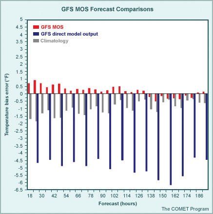
The correct answer is (b).

In the above case, the GFS MOS exhibits a warm bias at the shorter forecast projections and a cold bias at the extended projections (after the 132-hour forecast). Notice that both the direct model output (2-meter temperatures) and climatology exhibit strong cold biases at all forecast hours. Recall that the MOS technique accounts for both systematic model errors as well as decreased forecast accuracy at extended projections. In this case the cold bias seen in GFS direct output (shown in blue) is a systematic error, which would have been accounted for in the development of the MOS equations (provided that the GFS model used in development exhibited a similar bias). In addition, the GFS 2-meter temperatures (which are being used here for comparison) may not have been the optimal predictor used in the development of the MOS equations for the surface temperature forecasts. Remember that some model fields are not forecast well, and may not carry much weight in the development of the equations (and the MOS forecast itself). Finally, at extended projections, climatology for some predictors (such as temperature) tends to produce stronger statistical relationships with the predictand and thus carries more weight than other predictors (such as model data). Alternatively, if climatology were not an explicit predictor, the equations at the extended range projections would tend toward the mean of the developmental sample. Thus if that period of time happened to be warmer than normal, MOS would exhibit a cold bias. In the above example, the cold bias seen at extended lead times reflects the increased weight of climatology at the longer lead times.

Please make a selection.

Summary and Operational Tips

In the following summary and list of tips, most important items are put in bold type.

1. SG can provide accurate and objective forecast information that improves upon direct model output by:

• Removing systematic model errors and accounting for error growth with forecast projection (MOS only)
• Producing output variables that are not available from direct model output (such as visibility and thunderstorm parameters)
• Producing measures of confidence that specific weather events will occur (i.e., probability forecasts)

2. The procedures used to develop SG forecast equations influence the accuracy and usefulness of SG output.

• SG relationships are designed to fit most cases, assuming a normal distribution (±2SD).
• In skewed climate regimes, or extreme cases, such as droughts or extremely warm periods, SG forecasts will have little accuracy.

3. Some important considerations regarding the developmental datasets include:

• The length and period of the developmental sample is crucial. With a larger sample size it is more likely that rare (outlier) events will be included in the development of the forecast equations.
• Physically meaningful variables must be used to relate forecast variable to predictor.
• It is important to recognize the predictability of model variables (must select variables that provide useful forecast information and that can be forecast well by the model).
• PP does not include model forecast data in the development of regression equations. Therefore, PP guidance accuracy is susceptible to systematic model errors and degraded model accuracy with lead time.
• MOS does include model forecast data in the development of regression equations. Thus it is susceptible to changes to the operational models.
• Reducing the systematic error component of direct model output can result in degraded SG accuracy (remember that any change to the model suite requires redevelopment of the equations!).
• Increased model resolution may not improve SG, since data may be smoothed before developing SG products.

Additional Strengths, Weaknesses, and Use of SG

1. The role of forecaster experience is and should be paramount in determining the degree of reliance to be placed on MOS guidance numbers. MOS guidance is just guidance and should NEVER be taken at face value without careful consideration of all the available data. Consider the following:

• While MOS will correct for systematic bias overall, it will not correct for regime-dependent systematic biases (such as cold air damming). In these situations, SG output may not be reliable.
• SG output will have difficulty in resolving the same features that synoptic-scale NWP models cannot resolve (mesoscale and rare events, such as tropical storms, heavy precipitation, and tornadoes). When mesoscale features are expected to play a significant role and extreme or unusual events are expected, do not rely on SG output because it will be inaccurate.

2. SG output for some predictands may tend toward climatology at the medium and long-range (remember, that is done to account for degraded model accuracy at increased lead-time).

3. Conversely, observed weather elements are only used in the short-range (for some parameters, such as temperature, out to 36 hours).

Model Assessment Tools

* Purpose of Model Assessment Tools

Model assessment has traditionally been subjective, with the forecaster building upon experience to develop opinions about model accuracy. This can be done via simple, on-the-fly comparisons of model output to graphical analyses, satellite imagery, and surface and upper-air data plots. However, these comparisons can be misleading since they often contain personal biases and impressions.

As models become more complex and change more frequently, a more objective means of evaluating model performance is required, both to remove specific biases and to assess the impact of model changes on correcting known errors. Model accuracy assessment tools, also called model diagnostics or model verification, have evolved to provide an objective measure of model skill that can be used by forecasters.

In this section, forecasters will learn to make better use of objective evaluations of model performance through understanding and applying

• Total, systematic and random error measures
• Special error measures such as vector error and spatial measures
• Temporal and spatial domains

* Objective Assessment of Model Accuracy

In its most ideal form, the objective assessment of model accuracy can be thought of as a simple comparison of the model forecast and atmospheric truth as defined by the following.

In reality, this comparison is constrained by the limitations of model forecasts and the representation of atmospheric truth, which will be discussed further in a later sub-section.

* Defining Model Errors

Statistical measures generated from the objective comparison of model forecasts and atmospheric truth can provide a convenient means of describing and summarizing model accuracy. The sources of model forecast errors that define this accuracy can have both systematic and random components.

Total error summarizes the magnitude of all of the errors in the forecast—both the systematic and random components. While the total error can provide a more complete assessment of the amount of error, it is difficult to decipher the contributions from the systematic and random components. One can get more insight into the cause or source of an error by examining each component individually. Therefore, total error measures should be used in conjunction with systematic and/or random error measures.

Systematic errors are repeatable over time and may be caused by factors specific to a model or the verification method. For example, a model may consistently forecast overly cold surface temperatures because of a misrepresentation of model terrain or a problem in the radiation scheme. Systematic errors have consistent magnitudes that may be easily identifiable. They can be accounted for subjectively and even corrected through additional model development.

Random/non-systematic errors arise from our inability to completely measure the atmosphere or predict periodic changes in it. For example, popcorn convection on some summer afternoons can generate random errors since it often occurs randomly over an area and largely on a scale that cannot be depicted. Although random errors are unpredictable and cannot be easily corrected, they can be described mathematically and their effect on the forecast estimated statistically. Random errors provide a measure of confidence (or lack of it) that can be expected for a forecast.

In the next sub-section, you'll learn about statistical measures that address these error sources as well as those intended to assess spatial accuracy.

Statistical Measure of Total, Systematic, and Random Error

Different statistical measures can be used to assess each of the sources of model forecast error (total, systematic, and random). The most common examples are shown below. Click each type of measure (RMSE/MAE, Bias, and Standard Deviation) for more information.

Notice the following in the example:

• The bias error (systematic error) is shown as a consistent offset from the forecast
• The random error is shown as inconsistent variations about the forecast
• The total error is a combination of the contributions of both error types

These error measures work well for forecasts of temperature, geopotential heights, mean sea-level pressure, wind speed, and precipitation (to a degree). However, special measures are needed for:

• Vector parameters, such as wind (click for information on RMS vector error)
• Pattern matching to measure spatial accuracy. These measures are very useful for evaluating precipitation forecasts. They are discussed in more detail on the following page

RMSE/MAE

Root mean square error (RMSE) is the square root of the average of the individual squared differences between the forecast (f_n) and observation (o_n), where N is the total number of forecast comparisons.

Squaring this difference forces RMSE to weight both positive and negative errors equally, thus making RMSE a measure of total model error. Remember, as a total error measure, RMSE includes both systematic and random components, which can be separated out using systematic and random error measures such as Bias Error and Standard Deviation.

RMSE is often used to evaluate the error magnitude in a forecast of temperature, winds, and heights.

Mean absolute error (MAE) is the average of the absolute value of the difference between the forecast (f_n) and observation (o_n), where N is the total number of forecast comparisons. Taking the absolute value of this difference forces MAE to weight both positive and negative errors equally, thus making MAE a measure of total model error.

MAE is used to evaluate the error magnitude in a forecast of temperature, winds, and heights.

back to image

Bias Error

Bias error (BE) is the average of the difference between the forecast (f_n) and observation (o_n), where N is the total number of forecast comparisons. Because BE lacks a squared or absolute value term, cancellation of individual positive and negative errors is allowed, leaving only the excess, systematic error.

Bias error is often used to evaluate the magnitude of over or underforecasting of variables such as temperature, wind, height, etc. Negative values represent an underforecast, positive values represent an overforecast, and a value of zero means there is no bias.

back to image

Standard Deviation

Standard deviation (SD) is the square root of the average squared difference between the forecast error (e_n = f_n - o_n) and the mean forecast error (ē), where N is the total number of forecast comparisons and

• f_n denotes a specific forecast
• o_n denotes a specific observation

SD is used to measure the amount of variability in the forecast of meteorological variables. The higher the value of the SD, the higher the forecast variability. It can be shown statistically that approximately 67% of the time the random component of the total model error will lie within one standard deviation and 95% of the time within two standard deviations. Thus, SD can be used as a gauge of the expected range of the random or non-systematic contribution to the total forecast error, although the exact magnitude of the random error will vary widely (and can change sign) from case to case.

back to image

RMS Vector Error

Root mean square vector error (RMSVE) is simply the RMSE applied to the magnitudes of the forecast and observed vector components. In the above example, RMSVE is calculated for horizontal winds, using the square root of the sum of the squared differences between the magnitudes of the forecast (u_f and v_f) and observed (u_o and v_o) wind components. Recall that the u and v vectors correspond to the east-west and north-south components of the wind, respectively.

back to image

* Spatial Measures

Statistical measures can also measure spatial accuracy, highlighting the correct pattern and placement of a particular parameter. Such measures include the following. Click each for more information.

• Threat score
• Equitable threat score
• Correlation
• Anomaly correlation

Threat score

Threat score (TS) is a measure of the correct placement and timing of a forecast for a particular event. The overlap between forecast (F) and observation (O) for an occurrence is represented as a hit (H). TS compares the size of the correctly forecast area to the total area where the event was either predicted or observed.

TS is often calculated for a threshold amount, which is the hit-rate for a particular event exceeding a specific value. In the case of precipitation, this may be the score for forecasted precipitation amounts exceeding a threshold of 0.1 in. over a period of time (see example below). TS values may range from 0.0 to 1.0, where a score of one represents a perfect forecast and a score of zero indicates no skill.

In the above example, the filled contour intervals represent forecasted six-hr precipitation totals. The small circles represent equally spaced observations over the same period, where filled circles indicate observed precipitation. In this case, the forecast was for four sites to receive precipitation greater than or equal to 0.10 in., while in reality eight sites observed amounts equal to or exceeding that threshold (0.10 in). There were only three sites that observed precipitation amounts greater than or equal to 0.10 in. that were coincident with the forecast.

The threat score for this case (as calculated for the 0.10-in. threshold) is 0.33. Note that the observations used in the calculation actually measured higher amounts than the indicated threshold (0.25, 0.25, and 0.50 in.). Remember that TS is a measure for all amounts exceeding a given threshold and does not represent the skill of a forecast for this amount specifically. Keep in mind that this example is an ideal case with equally spaced observations and that in reality this is seldom true.

Equitable threat score

Equitable threat score (ETS) is similar to TS, where the overlap between forecast (F) and observation (O) for an occurrence is represented as a hit (H). However, ETS additionally accounts for the random chance (C) of a correct positive forecast. (TS may reward correct forecasts generated purely by chance and can be misleading.) Chance is defined as C = F x O/N, where N equals the total number of observations verified. Recall that like TS, ETS values equal to 1.0 represent perfect forecasts, while values near or equal to zero represent forecasts with little or no skill. Unlike TS, ETS may have negative values that represent forecast skill less than that of random chance (ETS = 0). ETS values are always lower than TS values.

Correlation

Correlation is a measure of the "degree of fit," or similarity, between forecast and observed patterns. Correlation values range between -1 and 1, where one represents perfect correlation and zero is no correlation. Correlation measures are best used for continuous wave patterns such as geopotential heights. Correlation is calculated over N locations, where f denotes forecast and o denotes observation.

In the graphic above, comparisons of simple wave patterns illustrate closely correlated (a), negatively correlated (b), and non-correlated functions (c).

Anomaly correlation

Anomaly correlation (AC) is a measure of the similarity between forecast and observation patterns using anomalies (usually departures from the climatological mean) for a particular parameter. AC is best used in global regimes, where the slowly changing portion of flow (long-waves) dominates and yet does not have a major effect on the weather. By removing the longest waves (climatology) and examining the smallest-scale features (anomalies), AC can focus on the significant patterns.

Forecast accuracy using AC is generally evaluated with respect to an established reference value. AC values equal or nearly equal to 1.0 indicate a perfect or near perfect forecast (similar forecast and observation anomaly patterns), while those below the reference value of 0.6 are typically regarded as having little or no value.

Anomaly correlation is calculated over N locations, where

• f_n denotes forecast
• o_n denotes observation
• C_n denotes the climatological mean of the observed parameter (o_n)

* Limitations and Impacts on Verification

Recall the idealized definition of objective accuracy assessment presented earlier:

As we mentioned, the objective assessment of model accuracy is constrained by the limitations of the model forecasts and the representation of atmospheric truth. Specifically

• Model forecasts represent the atmosphere as a discrete array of area-averaged values as opposed to the continuous fields found in the real world
• Atmospheric truth, against which forecasts are compared, is represented by observations and analyses of the atmosphere. No matter how sophisticated these observations and analyses become, they will never represent the atmosphere perfectly

* Limitations of Gridded Model Forecasts

How models and observations/analyses represent the atmosphere contributes to model forecast errors and detracts from the reliability of model assessment tools.

Techniques and Data Sources of Model Assessment Tools

The goal of model assessment is to verify how well the model predicted the state of the atmosphere. To do this, one must not only understand the strengths and limitations of the model being evaluated, but also the accuracy and applicability of the verification data.

Traditionally, model assessment tools use the following techniques and data sources to represent atmospheric truth, no one of which is clearly superior.

• Model analyses
• Independent objective analysis
• Point observations

These techniques and data sources are explored on the following pages.

Model Analyses

Model analyses are designed to minimize forecast error growth within a modeling system rather than represent atmospheric observations as closely as possible. Model analyses typically present a somewhat smoother version of the actual atmospheric field.

Model analyses are usually generated by blending a first-guess field with an observational data set. The first guess may be obtained from a previous forecast or from forecast data from another model.

Model analyses incorporate multiple types and sources of observations and may have excellent spatial and temporal resolution. But they are dependent upon the number and quality of observations passed into the analysis package. Missing observational data (such as those for extreme events rejected by the analysis' quality control system) can seriously hamper the analysis and cause the atmosphere to be misrepresented. If the analysis is too heavily influenced by the first guess, the model will be validating itself.

Remember that model data (both forecast and analyses) represent an area average at each grid point. Using a model's analysis in accuracy assessment can be very useful, particularly when comparing like-types of data. (If they're from the same model, the analysis represents the same area averages as the forecasts.) However, using model analyses can be problematic and unrepresentative, especially when

• The resolutions of the analysis and forecast are not well matched (i.e., different resolution grids represent different area averages)
• The accuracy assessment generated from one model (using its own analyses) is compared against measures from another (using a different model-specific analysis), which makes the comparison inconsistent

Independent Objective Analysis

Independent objective analysis data sets are generated solely from observations via an analysis system. (There is no model first guess.) These gridded data sets can incorporate observations from multiple sources and may have excellent spatial and temporal resolution.

Point Observations

Point observations are direct measurements of the atmosphere at discrete points. Although they represent the most simple and straightforward sampling of the atmosphere, they are limited by two significant sources of errors:

• Instrument errors related to the observing system. (The number of errors can, in many cases, be quite high)
• Errors of representativeness (how well a point observation represents the state of the atmosphere around a particular location). Point observations, such as radiosonde data, are typically limited spatially and temporally and may not be a random sampling of the atmosphere

The fact that model forecasts are represented as area averages over grid boxes further complicates the comparison of model forecasts with point observations. Model forecast grid box averages are not synonymous with the point observations used for comparison (see example below). To compare model forecasts to observations, the model data must either be interpolated to the observation point, taken from the nearest grid-point, or the data within each grid box must be averaged.

The Right Tools at the Right Time

Several strategies can help forecasters make intelligent use of statistical measures as objective model assessment tools.

• Understand the types of errors being measured - what is correctable (systematic errors) and what is not correctable (random errors)
• Define the forecast problem at hand. As the graphic below shows, a one-day versus seven-day forecast can require a different focus on parameters, time scales, and spatial scales, and will be affected by changing weather regimes differently

The following pages explore these strategies and some of the tools that can be used to objectively address the forecast problem in more detail.

Impact of Total Error Measures

Below is an example illustrating the impact of RMSE as a total error measure. It shows 700-hPA temperature RMSEs for a model initialization (F000) through forecast hour 48.

Bias (Systematic) Error Example

Below is the corresponding 700-hPA temperature bias errors BEs or the model initialization (F000) through forecast hour 48.

Standard Deviation (Random) Error Example

Below is the corresponding 700-hPA temperature SDs for the model initialization (F000) through forecast hour 48.

Impact of Temporal Period and Spatial Domain

Statistics generated over long time periods mask errors specific to smaller timescales, washing out the signatures of individual errors (i.e., they can minimize the effects of random errors in specific regions).

Statistics generated over shorter time periods are more susceptible to (and even dominated by) errors specific to localized regimes and may not be representative of overall model performance. However, these measures are useful in highlighting accuracy with respect to regimes on similar time scales. For example, statistical measures generated over three to five days can be used to address errors associated with specific weather regimes, such as upper-level ridging. In situations of rapidly changing regimes, even short period-averaged statistics may be misleading. Knowledge of the current weather and the performance of the model at upstream locations is critical.

Statistics generated over large domains, such as the Northern Hemisphere, mask smaller-scale errors associated with regions or locations. Such measures are more likely to highlight model errors that are independent of specific regions.

Statistics generated for smaller regions or locations isolate errors associated with those areas. For example, statistics generated over the Rocky Mountains or the Gulf Coast are more specific to those regions and useful to forecasters than measures generated over the whole domain.

Combinations of time and spatially averaged statistics are very useful.

* Impact of Single Forecast Statistical Measures

Statistical measures generated from forecast comparisons from an individual model run, with no temporal averaging, can be used to address the accuracy of the current model initialization as well as recent forecast performance. Such measures consist of statistics at individual locations or averaged over spatial domains.

Since single-forecast statistical measures are not averaged over time, they are much more sensitive to model errors with respect to specific weather systems or regimes of similar period and scope. Therefore, knowledge of current and expected weather is crucial. Expected weather changes can make previous or current statistical measures inapplicable. Individual forecast assessments are also very susceptible to problems within model analyses.

Diagnosing Near-term Model Performance on the Local Level

Model Assessment Tools Summary

Ideally, the process of objective model accuracy assessment is defined as:

The sources of model forecast error that define this accuracy can have both systematic and random components that can be quantified using statistical measures.

• Total errors consist of both systematic and random components, making them difficult to separate and interpret individually
• Systematic errors are repeatable errors that may be caused by model specific factors and can be corrected for
• Random errors are unpredictable, arising from an inability to precisely predict or measure the atmosphere. Random errors cannot be easily corrected for but their estimated magnitude and influence can be estimated statistically and provide a "window of confidence " for the forecaster

Statistical measures are available to assess the sources of systematic, random, and total model forecast errors. In addition, special measures are used to evaluate spatial accuracy.

• Root mean square error (RMSE) and mean absolute error (MAE): Measure total model forecast error
• Bias error (BE): Measures systematic model forecast error
• Standard deviation (SD): Measures random model forecast error (range of confidence)
• Threat score (TS), equitable threat score (ETS), correlation, and anomaly correlation (AC): Measure model forecast spatial accuracy (correct timing and placement)

Statistical measures averaged over spatial and temporal domains are powerful tools that allow the focused measurement and interpretation of model accuracy with respect to specific forecast problems, including measures of "correctibility" (using systematic error measures) and forecast confidence (using random error measures).

For information on the assessment tools used for some of the current operational models, see the Operational Models Encyclopedia.

References

Post-Processing

Benjamin, S.G., K.J. Brundage, and L.L. Morone, Cited 2000: Implementation of the Rapid Update Cycle Part I: Analysis/Model Description. NOAA/NWS Technical Procedures Bulletin, NOAA/ERL Forecast Systems Laboratory, Boulder, CO, 1994.

Carr, F.H., 1988: Introduction to Numerical Weather Prediction Models at the National Meteorological Center. University of Oklahoma, 63 pp.

Petersen, R.A., and J.D. Stackpole, 1989: Overview of the NMC production suite. Wea. Forecasting, 4, 314-322.

Ross, B.B., 1986: An overview of numerical weather prediction. Mesoscale Meteorology and Forecasting, P.S. Ray, Ed., Amer. Meteor. Soc., 720-751.

Treadon, R., 1993: The NMC Eta Model Post Processor: A Documentation. NMC Office Note No. 394, 42 pp.

Statistical Guidance

Carter, G.M., J.P. Dallavalle, and H.R. Glahn, 1989: Statistical forecasts based on the National Meteorological Center's numerical weather prediction system. Wea. Forecasting, 4, 401-412.

Dallavalle, J.P., 1996: A perspective on the use of model output statistics in objective weather forecasting. Preprints Fifteenth Conf. on Weather Analysis and Forecasting, Norfolk, VA, Amer. Meteor. Soc., 479-482.

Glahn, H.R., 1985: Statistical weather forecasting. Probability, Statistics, and Decision Making in the Atmospheric Sciences, A.H. Murphy and R.W. Katz, Eds., Westview Press, 289-335.

Glahn, H.R., and D.A. Lowry, 1972: The use of model output statistics (MOS) in objective weather forecasting. J. Appl. Meteor., 11, 1203-1211.

Glahn, H.R., K. Gilbert, R. Cosgrove, D. P. Ruth, and K. Sheets, 2009: The Gridding of MOS. Wea. Forecasting, 24, 520–529.

Marzban, Caren, S. Sandgathe, and E. Kalnay, 2006: MOS, Perfect Prog, and Reanalysis. Mon. Wea. Review, 134, 657–663.

Wilks, D.S., 1995: Statistical Methods in the Atmospheric Sciences. Academic Press, 467 pp.

Model Assessment Tools

Baldwin, M. E., and S. P. Hrebenach, 1998: Experiments with bias-corrected temperature guidance using NCEP's mesoscale Eta model. Preprints, 16th Conf. On Weather Analysis and Forecasting, Phoenix, AZ, Amer. Meteor. Soc., 388-389.

Lorenz, E. N., 1969: Atmospheric predictability as revealed by naturally occurring analogues. J. Atmos. Sci., 26, 636-646.

Mao, Q., R.T. McNider, S.F. Mueller, and H. H. Juang, 1998: An optimal model output calibration algorithm suitable for objective temperature forecasting. Wea. Forecasting, 14, 190-202.

Nutter, P. A., and J. Manobianco, 1998: Evaluation of the 29-km Eta Model. Part I: Objective verification at three selected stations. Wea. Forecasting, 14, 5-17.

Nutter, P. A., and J. Manobianco, 1998: Evaluation of the 29-km Eta Model. Part II: Subjective verification over Florida. Wea. Forecasting, 14, 18-37.

Panofsky, H. A., and G. W. Brier, 1965: Some Applications of Statistics to Meteorology. Pennsylvania State University, University Park, 224 pp.

White, W. G., J. Paegle, W. J. Steenburgh, J. D. Horel, R. T. Swanson, L. K. Cook, D. J. Onton, and J. G. Miles, 1998: Short-term forecast validation of six models. Wea. Forecasting, 14, 84-107.

Wilks, D.S., 1995: Statistical Methods in the Atmospheric Sciences. Academic Press, 467 pp.

Contributors

COMET Sponsors

The COMET^® Program is sponsored by NOAA National Weather Service (NWS), with additional funding by:

• Air Force Weather (AFW)
• Australian Bureau of Meteorology (BoM)
• European Organisation for the Exploitation of Meteorological Satellites (EUMETSAT)
• Meteorological Service of Canada (MSC)
• National Environmental Education Foundation (NEEF)
• National Polar-orbiting Operational Environmental Satellite System (NPOESS)
• NOAA National Environmental Satellite, Data and Information Service (NESDIS)
• Naval Meteorology and Oceanography Command (NMOC)

Project Contributors

Principle Science Advisors

• Dr. Ralph Petersen — NOAA/NCEP/EMC (retired)
• Kirby Cook — NOAA/NWS
• Dr. William Bua — UCAR/COMET
• Dr. Stephen Jascourt — UCAR/COMET

Senior Project Manager

• Dr. Gregory Byrd — UCAR/COMET

Project Leads

• Dr. William Bua — UCAR/COMET
• Dr. Stephen Jascourt — UCAR/COMET

Instructional Design

• Bryan Guarente — UCAR/COMET
• Tsvetomir Ross-Lazarov — UCAR/COMET

Graphics/Interface Design

• Steve Deyo — UCAR/COMET
• Brannan McGill — UCAR/COMET
• Heidi Godsil — UCAR/COMET

Multimedia Authoring

• Bruce Muller — UCAR/COMET
• Dan Riter — UCAR/COMET

COMET HTML Integration Team 2020

• Tim Alberta — Project Manager
• Dolores Kiessling — Project Lead
• Steve Deyo — Graphic Artist
• Gary Pacheco — Lead Web Developer
• David Russi — Translations
• Gretchen Throop Williams — Web Developer
• Tyler Winstead — Web Developer

COMET Staff, October 2009

Director

• Dr. Timothy Spangler

Deputy Director

• Dr. Joe Lamos

Administration

• Elizabeth Lessard, Administration and Business Manager
• Lorrie Alberta
• Michelle Harrison
• Hildy Kane

Hardware/Software Support and Programming

• Tim Alberta, Group Manager
• Bob Bubon
• James Hamm
• Ken Kim
• Mark Mulholland
• Wade Pentz, Student
• Jay Shollenberger, Student
• Malte Winkler

Instructional Designers

• Dr. Patrick Parrish, Senior Project Manager
• Dr. Alan Bol
• Lon Goldstein
• Bryan Guarente
• Dr. Vickie Johnson
• Tsvetomir Ross-Lazarov
• Marianne Weingroff

Media Production Group

• Bruce Muller, Group Manager
• Steve Deyo
• Seth Lamos
• Brannan McGill
• Dan Riter
• Carl Whitehurst

Meteorologists/Scientists

• Dr. Greg Byrd, Senior Project Manager
• Wendy Schreiber-Abshire, Senior Project Manager
• Dr. William Bua
• Patrick Dills
• Dr. Stephen Jascourt
• Matthew Kelsch
• Dolores Kiessling
• Dr. Arlene Laing
• Dr. Elizabeth Mulvihill Page
• Amy Stevermer
• Warren Rodie
• Dr. Doug Wesley

Science Writer

• Jennifer Frazer

Spanish Translations

• David Russi

NOAA/National Weather Service - Forecast Decision Training Branch

• Anthony Mostek, Branch Chief
• Dr. Richard Koehler, Hydrology Training Lead
• Brian Motta, IFPS Training
• Dr. Robert Rozumalski, SOO Science and Training Resource (SOO/STRC) Coordinator
• Ross Van Til, Meteorologist
• Shannon White, AWIPS Training

Meteorological Service of Canada Visiting Meteorologists

• Phil Chadwick
• Jim Murtha