Introduction
Imagine you are the lead forecaster at the National Weather Service’s (NWS) Monterey, CA Weather Forecast Office (WFO), comparing the Real-Time Mesoscale Analysis/Un-Restricted Mesoscale Analysis (RTMA/URMA) and MatchObsAll temperature analyses in the BIg Sur area of the Central California coast.
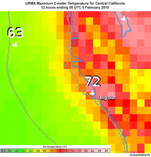
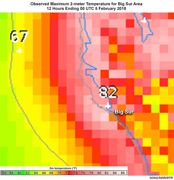
URMA maximum 2-meter temperature analysis (°F) and observed maximum 2-meter temperature analysis (°F), 4 February 2018. For both graphics, the dark grey line off the coast represents the outer boundary of WFO responsibility for marine forecasts. The blue line is the land-sea boundary in AWIPS2, and the lighter gray represents the actual land-sea boundary.
“We’ve seen this kind of difference around Big Sur every time we have an offshore wind event,” you think. “It’s a big tourist area, so temperature errors have a significant impact.”
You ask your Science and Operations Officer (SOO) about the source of the difference. “Well, the MatchObsAll tool draws close to the observations,” she says. “While the RTMA/URMA also uses observations, it’s starting point (or first guess) blends the current 1-hour 3km HRRR forecast and the most recent (00, 06, 12, or 18 UTC) NAM-Nest forecast. Terrain, coastline location, the forecast-observation difference, and observation quality relative to the first guess are then used to complete the analysis.”
You note, ”Because the RTMA/URMA depends on the first guess, observations, terrain, and coastline location, problems with any of these could result in big analysis errors. The Big Sur observation is good, but our rugged terrain often results in features being missed in the first guess. If a feature isn’t in the first guess, it’s hard to get it into the analysis, even if you have an observation that captures it. Also, I’ve been hearing about problems with inconsistencies with the terrain and the coastlines, and even a good first guess won’t help with that.”
Introduction » Terrain Inconsistencies
You wonder, “Which products are affected by this terrain and shoreline inconsistency? How does this problem affect the forecast process?”
Question
Do the following NWS products use terrain or shorelines in their development? Choose True or False.
Direct model output (e.g. GFS and NAM) does not require terrain to be gridded to the desired resolution. Gridded MOS uses terrain in regridding individual station GFS MOS data to 2.5-km resolution. The NBM indirectly uses terrain because its components are bias corrected using URMA, which is terrain-dependent.
To reduce the problems related to disparate terrain grids, the NWS is adopting a single Unified Terrain for use in the RTMA/URMA, downscaling NWP grids to create the NBM, and in the Advanced Weather Interactive Processing System (AWIPS) Graphical Forecast Editor (GFE). Since early 2018, the RTMA/URMA and NBM have been using the new Unified Terrain. However, their data still need to be imported into the AWIPS GFE, which currently has an older terrain data set (as of August 2018).
In this lesson, we will examine the terrain and shorelines used in the following:
- The Real-Time Mesoscale Analysis (RTMA), which combines two short-range forecasts (HRRR and NAM Nest) for a “first guess” starting point, downscales the result to 2.5 km, and then assimilates surface observations from near the analysis valid time. The result is the 2-dimensional (2D) RTMA analysis, which forecasters often use for situational awareness.
- The Un-Restricted Mesoscale Analysis (URMA), which extends the RTMA observation window to 6 hours to make a more complete 2D analysis. The URMA is used to verify National Weather Service (NWS) NWP models and other forecast products. Note that we will refer to the two analyses as the RTMA/URMA unless they need to be discussed separately.
- The National Blend of Models (NBM), which uses downscaled, bias-corrected, and performance-weighted NWP and statistical model components to create its blended products.
- The AWIPS Graphical Forecast Editor (GFE), where forecasters use forecast guidance to develop forecast grids for the National Digital Forecast Database (NDFD).
The Problems
Problems can result when different terrain data sets are used to create an analysis, downscale grids during postprocessing, or develop a gridded forecast using a system like AWIPS GFE. These problems can result from computational, input/output, and data storage errors, or from using different source data provided to create the terrain. There are more common problems however, that we will discuss in the following sections.
The Problems » Inconsistent Updating to New Data Sets
An operational weather service’s platforms may have different terrain and shoreline maps if those maps are not updated concurrently when new terrain data become available.
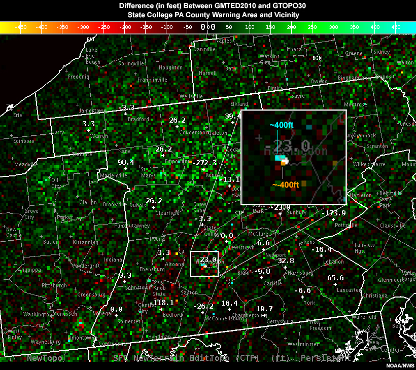
For example, the graphic below shows the difference between the new Unified Terrain and the terrain deployed in AWIPS GFE. In the zoomed-in box, the Unified Terrain is 400 feet lower in the orange box and 400 feet higher in the blue box. If either or both of these new elevations are not representative, the forecast variables will be incorrect, and forecasters will need to adjust them based on their knowledge of the area.
The Problems » Different Interpolation Methods
Interpolation of high-resolution source terrain and shoreline data to the analysis and downscaling grids can use different methods. We’ll briefly examine two common methods and see how using different methods on the same source data results in different terrain grids.
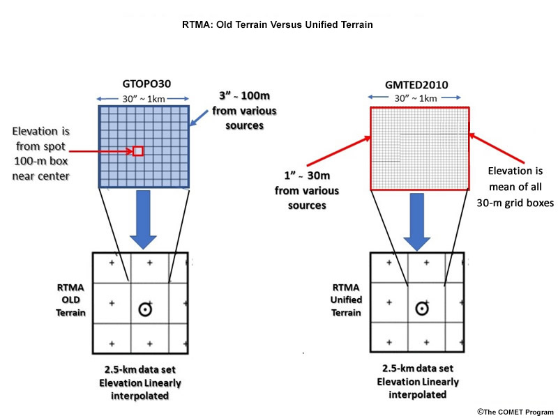
The graphic below shows the method used to create the previous version of 2.5-km terrain in the RTMA/URMA on the left, while the method used to create the Unified Terrain is on the right. The 100-m resolution source data used for GTOPO30 were updated for the GMTED2010, and made available at 30-m resolution.
- In the first step (top row), source data are aggregated to 1-km grid boxes.
- The second step (top row) is to choose the terrain height of the grid box. In the older version, the terrain height of a 100-m grid box near the middle of the larger grid box was chosen, while the mean value of all 30-m grid boxes was used for Unified Terrain.
- In the third step (bottom row), the 1-km data are interpolated using bilinear interpolation (a form of grid box averaging). Other methods include nearest neighbor (uses value from the nearest point) and polynomial interpolation. While not shown in the graphic, different interpolation methods will yield different results.
Left: Bilinear interpolation method used to create 2.5-km terrain. Right: Nearest neighbor method used to create 2.5-km terrain. Both start from a common 100-meter terrain height data set.
Question
Terrain data are used for plotting forecast guidance and creating a 2D analysis. Which of the following would create differences between the terrain heights for both functions? Choose all that apply.
Terrain height differences come from using different source terrains or assigning terrain height to a grid box using either different parts of the grid box or different aggregated grid boxes. Interpolating and aggregating source data does not by itself generate terrain differences.
The Problems » Terrain Contour Shape Inconsistencies in the RTMA
We’ve looked at how differences in terrain source data and interpolation techniques result in terrain inconsistencies in analysis and downscaling systems. Why do they matter? What impact do they have? The answers lie in the dependence of the RTMA/URMA analysis and NBM downscaling on terrain, and the import of the RTMA/URMA and NBM grids into the AWIPS GFE.
We’ll start with the RTMA/URMA analysis and see how it’s impacted by terrain inconsistencies from various sources.
Question
Which statements do you think accurately describe the RTMA/URMA’s dependence on terrain? Choose all that apply.
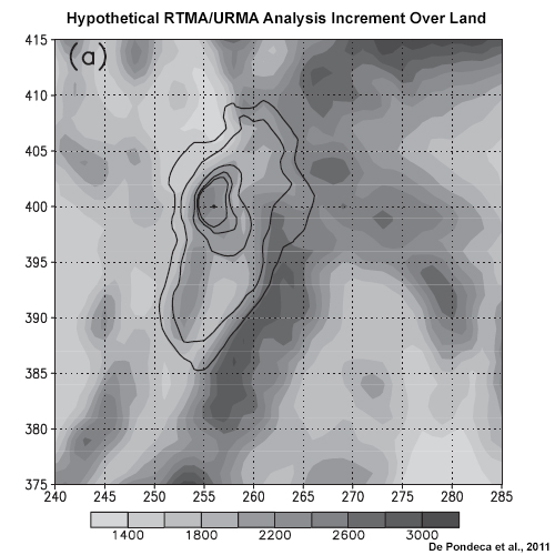
The effect of observations on the RTMA/URMA is a function of distance and the terrain. To illustrate this, the graphic below shows the terrain-dependent area of influence of an observation on the RTMA/URMA analysis. The area of influence gets stretched along terrain contours and narrowed in areas with strong terrain gradients (near the observation location). Therefore, if the terrain is incorrect, the observations’ area of influence will be incorrect.
Additionally, the RTMA/URMA’s 2.5-km resolution does a better job of capturing, for example, early morning cold pools resulting from radiational cooling in low-lying terrain than most NWP models. However, it will still misanalyze them if the terrain features that generate them are too small to be resolved by the 2.5 km grid.
Finally, the URMA is used to compute NBM component biases and RMSE, which implies NBM indirect dependence on terrain.
Shoreline data are usually separate from the terrain height data. As a result, shorelines may not correspond to mean sea level.
The Problems » Terrain Contours and Downscaled Data
The downscaling of model components used in the NBM also depends indirectly on the shape of the underlying terrain–through the use of the terrain-dependent RTMA/URMA to bias-correct model components. While we don’t show this here, discrepancies in the terrain result in discrepancies in the downscaled variables.
The Problems » Shorelines and the RTMA/URMA
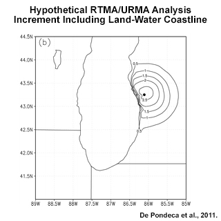
Shorelines have an important role in the RTMA/URMA analysis. Below is a hypothetical area of influence for an RTMA observation that includes a shoreline. The area of influence stops at the shoreline to reflect the different impacts of water versus land on the near-surface atmosphere. Shorelines shape the area of influence affecting the RTMA/URMA analysis first guess, so incorrect shorelines will lead to nearby analysis errors.
The Problems » Shorelines and Downscaled Model Data
Now we’ll explore some of the reasons why shorelines are important to downscaled NWP model data in the NBM, through use of the RTMA/URMA to perform bias-correction.
Question
You’re working in the Portland OR WFO in July and are in the process of creating your 2.5-km gridded forecast using the AWIPS GFE. You know that the GFE has slightly different shorelines than the 2.5-km NBM forecast data you’re importing. What impact might this have? Select the correct words to complete the sentences.
As of June 2018, there are two problems with shorelines. The first, which has significant impacts on weather variables, has to do with discrepancies between land and water grid boxes in the GFE, the NBM, and the URMA, which impacts how both the NBM and URMA data are downscaled to 2.5 km.
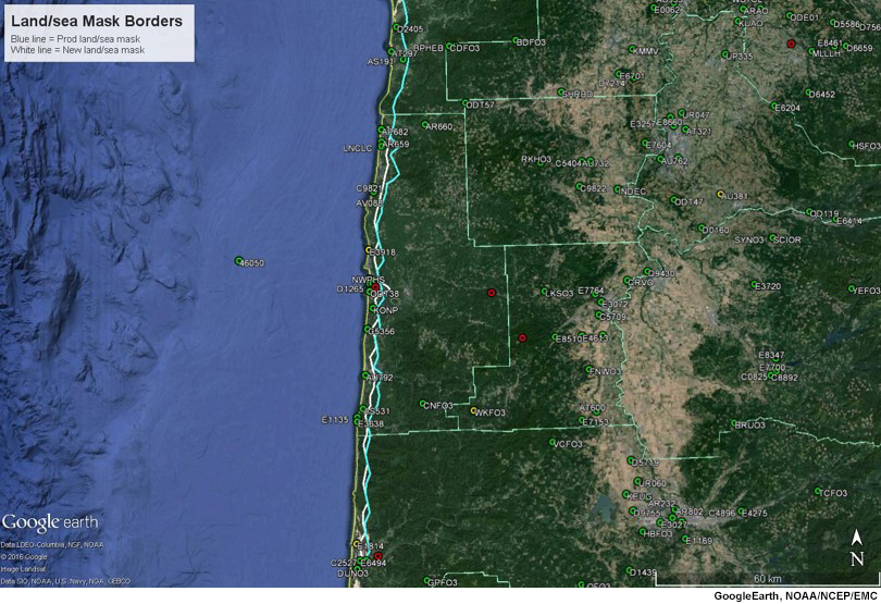
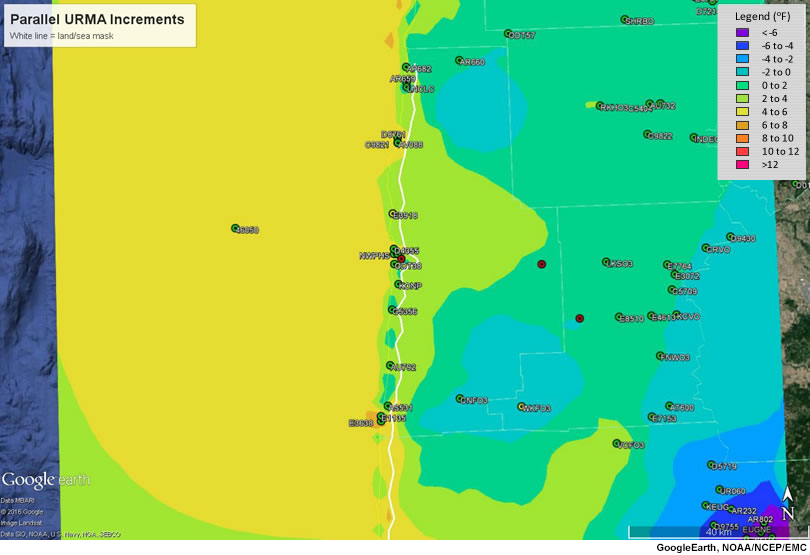
The following graphic from the Oregon coast shows an area with such a discrepancy. The blue line represents the old AWIPS GFE coastline, and the white line is the new Unified Terrain coastline, shifted slightly westward. Note that many stations are located west (offshore) of the designated shoreline, and some of them are considered ocean points for the URMA.
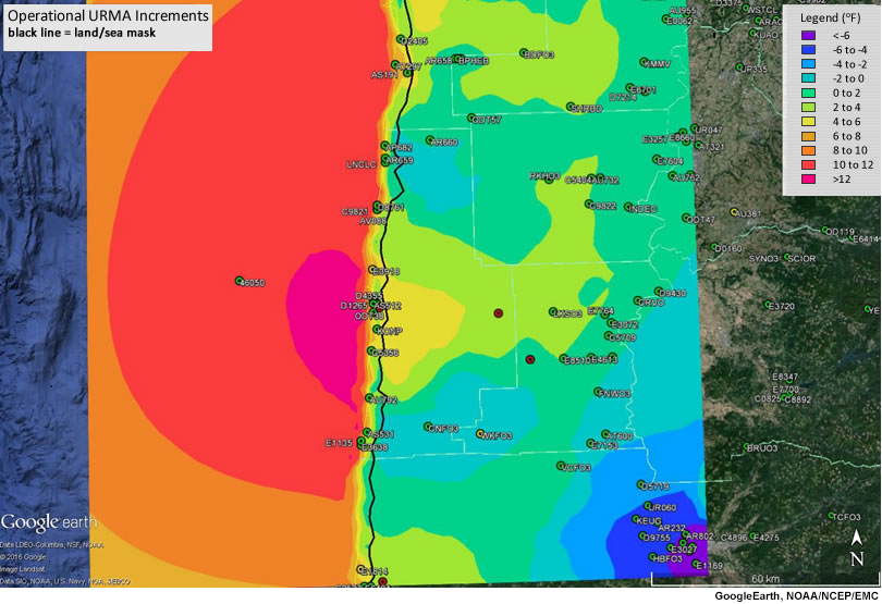
The consequences of land observations located on water points can be seen in the next graphic, showing the URMA analysis increments based on the old coastline. Large positive increments spread seaward from the coastline, because the influence of water and land increments both end at the water’s edge. The worst errors are found near a cluster of coastal land observations designated URMA water points, where analysis increments exceeding 12°F extend into the Pacific Ocean. Because water increments only apply to water points, these large increments do not affect land.
The new coastline was to mitigate these large errors over water points. Below we show the analysis increments that result.
The analysis increments, while still spreading seaward from the coastline, are mostly 4-6°F, with a small area of 6-8°F near a different group of coastal land points. While this represents a significant improvement, the portion over water is likely still too warm and covers too large an area.
The Problems » Shoreline versus Mean Sea Level
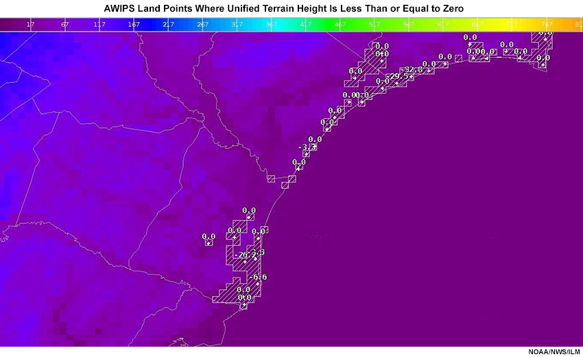
The other problem relates to the shoreline height being different from mean sea level, which results from the shoreline and terrain coming from different sources. The graphic below, comes from the Wilmington, North Carolina WFO. The hatched areas show land points with a terrain elevation less than or equal to zero. Where the topography is relatively flat, these discrepancies have little impact on the RTMA and the downscaled NWP forecasts used in the NBM; that’s because there are only small height differences between the Unified Terrain and mean sea level. Differences can become significant with rugged terrain at the shoreline, such as along the U.S. West Coast.
The Solution: Unified Terrain
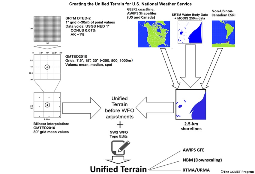
The solution to these issues is to use the same terrain height and shorelines in all analyses and downscaling systems that are dependent on terrain. The NWS Meteorological Development Lab (MDL) created the Unified Terrain to replace terrain and shorelines in the RTMA/URMA, NBM, and AWIPS data display system. Its source data are the Global Multi-resolution Terrain Elevation Data 2010 (GMTED2010, Carabajal et al., 2011), which were created at 1000-m, 500-m, and 250-m resolutions from an amalgam of these global and regional data sets:
- Global Digital Terrain Elevation Data (GDTED) from the Shuttle Radar Topography Mission
- Canadian elevation data
- Spot 5 Reference 3D data
- Ice, Cloud, and land Elevation Satellite (ICESat)
Shorelines come from the following sources:
- CONUS: NWS shapefiles, with MODIS data for some inland water bodies,
- Canada: NWS shapefiles and Great Lakes Environmental Research Laboratory (GLERL) data, and
- Mexico and other non-US territories: ESRI continent data.
As of June 2018, the Unified Terrain is used in the NBM and RTMA/URMA, but not yet in the AWIPS GFE. The shorelines, however, are now the same in the NBM, RTMA/URMA, and AWIPS GFE. This does not necessarily mean that RTMA/URMA represents the shorelines exactly, or that there have not been changes. For example, WFOs may alter shorelines to improve representativeness of nearshore land analyses and forecasts.
The diagram below shows the steps used to create the Unified Terrain. For more information, see this lesson page on Interpolation Methods.
The new Unified Terrain reduces the terrain height root mean square error (RMSE) compared to observed terrain height data by one-third to one-half over the previously used GTOPO30. Even so, large areas poleward of 60°N and 60°S need better terrain data. Improvements will be made in the future as better terrain data become available in polar regions.
The Solution: Unified Terrain » Finalizing the Unified Terrain and Shoreline for GFE
In the near future, NWS WFOs will be able to compare the Unified Terrain to those in the GFE within AWIPS. The Unified Terrain will be edited based on this comparison. Note that shorelines can be edited now through the AWIPS zone editing change process.
Question
Why do you think these state-of-the-art datasets need further editing? Choose all that apply.
Even at 2.5 km, terrain and shorelines may not be representative of important forecast locations, especially in areas of highly variable terrain. The WFOs will edit the Unified Terrain and shorelines to make them more representative at important observation points and population centers. The edits will be returned to the MDL, used to adjust the current Unified Terrain and land-water boundaries, and finally updated in the NBM, RTMA/URMA, and the GFE.
Impact of Unified Terrain
After the final Unified Terrain and shorelines are put into the RTMA/URMA, NBM, and AWIPS GFE, they will all work from the same terrain data set. For the RTMA/URMA, observational areas of influence will map in a way that’s consistent with terrain contours and shorelines in the NBM. For downscaling, bias correction, and NBM error-based component weighting, consistent terrain data will result in the same representation for each forecast location in an NWS WFO county warning area. Once the AWIPS GFE is working with the final Unified Terrain and shorelines, forecast grids, including the NBM, should not need to be adjusted to correct for representativeness errors resolvable at 2.5-km resolution. Recall that analysis increments are spread out over land based on terrain height. So better terrain may improve the area of influence of first guesses/analysis differences in the RTMA/URMA, and improved shorelines will better place the “sharpening” of the analysis increment at the water’s edge.
Limitations of 2.5-km Unified Terrain
Using Unified Terrain in the RTMA/URMA, NBM, and AWIPS GFE will not solve all terrain-related grid problems. That’s because some small meteorologically important features cannot be resolved by a 2.5-km grid, and because we cannot fully correct for errors in the first guess.
Limitations of 2.5-km Unified Terrain » Unresolved Terrain and Shorelines
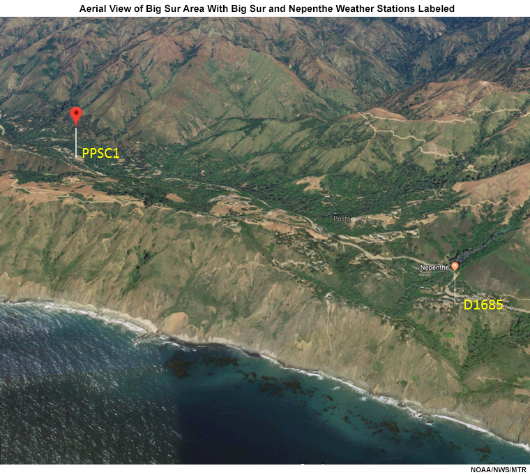
A 2.5-km resolution grid may be insufficient to resolve terrain features important to local weather. To illustrate, let’s go back to Big Sur and the Monterey, CA WFO. Look at this oblique aerial view from Big Sur. Two observing stations, separated by about 3.25 km, are a kilometer or less from the coastline.
Oblique Aerial
Topography
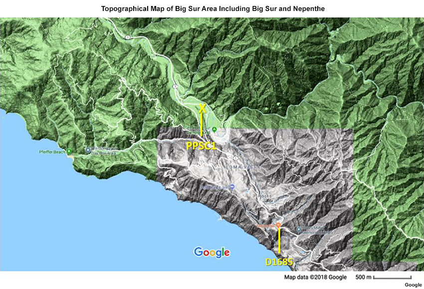
Station D1685 is open to the ocean at about 800’ above sea level, while station PPSC1 is on the Big Sur Valley floor at about 400’ and protected from marine influences by a ridge to its west. Temperatures can differ between the stations by as much as 15°F when flow is offshore.
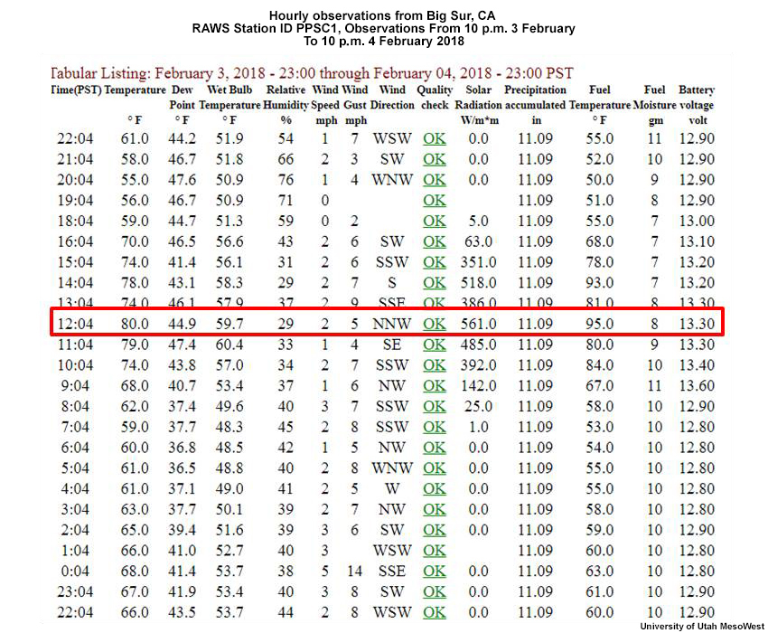
The hourly observations below are from PPSC1 on 4 February 2018 when it was as warm as 80°F at 12:04 p.m. PST (the high temperature of 82°F occured between hours). Click the second tab to compare them with the hourly observations from D1685, where it was only about 65°F at approximately the same time.
PPSC1 (Big Sur Valley)
D1685 (Coastal)
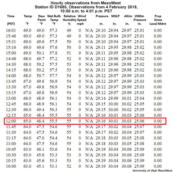
Do we have the terrain details necessary to get the temperatures correct in the URMA 2.5-km grid? Not a chance! In this case, both the terrain and the location of the shoreline impact the analysis grid.
We saw in the introduction how the URMA struggles to make a good analysis in this area. Now it is clear that the analysis error is also a problem of representativeness. The NBM, as a result, will also have difficulty with its forecasts, as the URMA is used to bias-correct and downscale the NBM components to 2.5-km (not shown).
Limitations of 2.5-km Unified Terrain » Bad Background Field/First Guess
As with any data assimilation system, a background or first guess field is taken from a short-range model forecast. For the RTMA, the starting point is a blend of the most recent available HRRR and the NAM CONUS Nest analyses. Observations then use the Unified Terrain to adjust the first guess to the best possible RTMA. It assumes that the first guess is a good starting point. But what if it isn’t?
Here’s an example from the southern Colorado Rockies from winter 2017-18. The terrain for the Wet Mountain Valley area, a frequent location for cold pools under favorable conditions, is found in the following graphic. Mountains of 13,000 to 14,000 feet are found to the valley’s east and west.
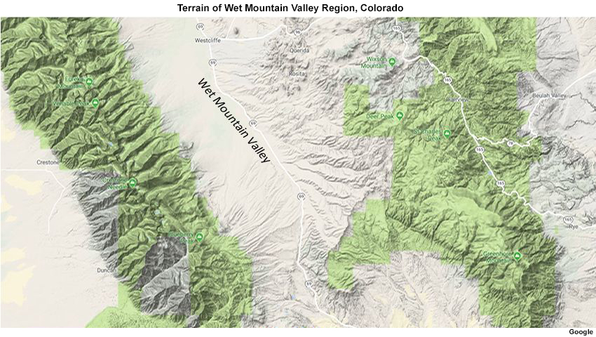
The WFO analyzed the observations using the Smarttool MatchObsAll, which draws close to the observations. Actual observations are in white.
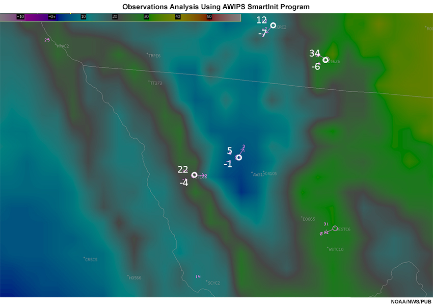
Observed temperatures in the center of the Wet Mountain Valley cold pool are near 0°F.
The RTMA analysis below uses the Unified Terrain to shape the area affected by first guess/analysis differences. The cold pool is almost nonexistent because the first guess did not capture it (not shown). The error could be due to insufficient resolution to depict a significant terrain feature or issues with near surface or other model physics. Or it just might be a bad observation.
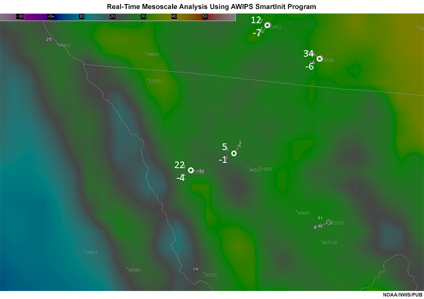
Each update to the RTMA/URMA is improved by changing the observational mix through quality control, improving the model used as the background field, or how the observations are distributed. Some of the errors shown in this lesson may have been partially corrected in recent updates. Even so, they show how the RTMA/URMA can be affected by the depiction of terrain and shorelines because of their impact on the analysis increments.
Conclusions
This lesson discussed issues related to using inconsistent terrain to create forecasts in the NBM and other forecast tools. From there, it described the Unified Terrain solution made from the GMTED2010 high-resolution terrain data set. Using the Unified Terrain in the RTMA/URMA, NBM, and GFE will produce a more accurate distribution of corrections to the RTMA/URMA first guess, improved depiction of contrasting weather elements across shorelines, and potentially better representation of terrain-dependent features. However, even with a consistent, accurate terrain data set, features too small to be resolved at the existing resolution will either be unrepresented or poorly represented, and a bad background field will be difficult to overcome.
You have reached the end of the lesson. Please complete the quiz and share your feedback with us via the user survey.
References
Carabajal, Claudia, David Harding, Jean-Paul Boy, Jeffrey Danielson, Dean Gesh, et al. Evaluation of the Global Multi-Resolution Terrain Elevation Data 2010 (GMTED2010) Using ICESat Geodetic Control. INTERNATIONAL SYMPOSIUM ON LIDAR AND RADAR MAPPING 2011: TECHNOLOGIES AND APPLICATIONS, 2011, 8286, pp.82861Y
University Corporation for Atmospheric Research, The COMET Program, 2010: Downscaling of NWP Data. Accessed 26 April 2018, https://www.meted.ucar.edu/training_module.php?id=794
University Corporation for Atmospheric Research, The COMET Program, 2012: Gridded Forecast Verification and Bias Correction. Accessed 26 April 2018. https://www.meted.ucar.edu/training_module.php?id=902
Contributors
COMET Sponsors
MetEd and the COMET® Program are a part of the University Corporation for Atmospheric Research's (UCAR's) Community Programs (UCP) and are sponsored by
- NOAA's National Weather Service (NWS)
with additional funding by: - Bureau of Meteorology of Australia (BoM)
- Bureau of Reclamation, United States Department of the Interior
- European Organisation for the Exploitation of Meteorological Satellites (EUMETSAT)
- Meteorological Service of Canada (MSC)
- NOAA's National Environmental Satellite, Data and Information Service (NESDIS)
- NOAA's National Geodetic Survey (NGS)
- National Science Foundation (NSF)
- Naval Meteorology and Oceanography Command (NMOC)
- U.S. Army Corps of Engineers (USACE)
To learn more about us, please visit the COMET website.
Project Contributors
Project Lead
- Dr. Bill Bua, UCAR/COMET
Instructional Design
- Dr. Alan Bol, UCAR/COMET
Science Advisors
- David Myrick, NOAA/NWS
- Jeffrey Craven, NOAA/NWS/MDL
- National Weather Service NBM Training Team
- Robert Ballard
- Randy Graham
- Jeff Hovis
- Eric Howieson
- Rebecca Mazur
- Mike Staudenmeier
- Brian Miretzky, NOAA/NWS
- Geoff Wagner, NOAA/NWS/MDL
Program Oversight
- Amy Stevermer, UCAR/COMET
Graphics/Animations
- Steven Deyo, UCAR/COMET
Multimedia Authoring/Interface Design
- Gary Pacheco, UCAR/COMET
COMET Staff, August 2018
Director's Office
- Dr. Elizabeth Mulvihill Page, Director
- Tim Alberta, Assistant Director Operations and IT
- Paul Kucera, Assistant Director International Programs
Business Administration
- Lorrie Alberta, Administrator
- Auliya McCauley-Hartner, Administrative Assistant
- Tara Torres, Program Coordinator
IT Services
- Bob Bubon, Systems Administrator
- Joshua Hepp, Student Assistant
- Joey Rener, Software Engineer
- Malte Winkler, Software Engineer
Instructional Services
- Dr. Alan Bol, Scientist/Instructional Designer
- Sarah Ross-Lazarov, Instructional Designer
- Tsvetomir Ross-Lazarov, Instructional Designer
International Programs
- Rosario Alfaro Ocampo, Translator/Meteorologist
- David Russi, Translations Coordinator
- Martin Steinson, Project Manager
Production and Media Services
- Steve Deyo, Graphic and 3D Designer
- Dolores Kiessling, Software Engineer
- Gary Pacheco, Web Designer and Developer
- Sylvia Quesada, Production Assistant
Science Group
- Dr. William Bua, Meteorologist
- Patrick Dills, Meteorologist
- Bryan Guarente, Instructional Designer/Meteorologist
- Matthew Kelsch, Hydrometeorologist
- Erin Regan, Student Assistant
- Andrea Smith, Meteorologist
- Amy Stevermer, Meteorologist
- Vanessa Vincente, Meteorologist