1. The Analysis Should Match Observations
- Misconception
- Observed Data vs Model Resolution and Physics: Observed Data
- Observed Data vs Model Resolution and Physics: Accounting for Discrepancies
- Assimilation Cycling
- Accountability in Action
- Test Your Knowledge
- Reality
1. The Analysis Should Match Observations » Misconception
In trying to produce the best possible NWP forecast, you might think that the model initial analysis should match exactly the observations used in that analysis, but you would be wrong.
Let's explore what's behind this counter-intuitive misconception.
The initial analysis comes from a complicated combination of the observations and a short range model forecast called the trial field (also referred to as the first guess field), and is designed to provide the best possible starting point for the forecast model. The analysis must account for such factors as differing accuracy of the various observing systems, the possibility of incorrect observations, and the relative importance of the trial field and the observations. The analysis must also be consistent with the model's own resolution and its own physics. For these reasons, the model initial analysis will differ somewhat from the observations.
1. The Analysis Should Match Observations » Observed Data vs Model Resolution and Physics: Observed Data
To illustrate why this is necessary, let's take a look at an example of several different observation types within a typical model grid. In the illustration we have a two-dimensional cross section of the three-dimensional model grid: the grid is composed of a multitude of rectangular boxes. Within the sample area enclosed by the grid, we find a number of different observing systems:
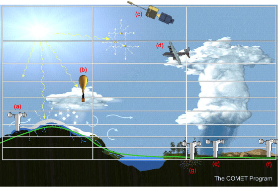
(a) A surface observing system (for example, from the synoptic network) where there is a sub-grid scale gradient in snow cover and topography, as well as in surface temperature.
(b) A radiosonde ascending through a sub-grid scale snow shower.
(c) A satellite measuring a particular radiance from an atmospheric layer which is thicker than the height of the individual grid boxes.
(d) An airplane measuring the sub-grid scale wind at the level of a cumulonimbus anvil.
Three additional surface observations in the same grid box:
- (e) one in the convective rain shaft;
- (f) one in the pre-convective area ahead of the cloud;
- (g) one in the post-convective area behind the cloud.
In general, the resolution of observations in the real atmosphere is different from the model's resolution, which means that features resolved by the model are "different" in some sense from the features resolved by the observing systems.
1. The Analysis Should Match Observations » Observed Data vs Model Resolution and Physics: Accounting for Discrepancies
In some cases there are features that the model can't resolve, but that the observations can. In other cases, the observing system samples a volume larger than the grid box resolved by the model. Furthermore, we mustn't forget that the trial field is always used in the analysis. The analysis considers the trial field to be, essentially, another type of data, with values available on the full three-dimensional grid.
Let's discuss some of these ideas in more detail:

- (1) Sample resolution in the atmosphere versus model resolution:
- The satellite measures average radiances over a deep layer in the atmosphere, while the model actually has better vertical resolution than the satellite is capable of sensing.
- (2) Consistency with model physics:
- The analysis will add moisture to reflect the observed humidity at an observation such as the one in the rain shower. However, if the model atmosphere tends to be too dry, then the model will simply dump out a lot of moisture during the first few time steps to dry itself out to the level required by its own physics.
- (3) Grid boxes containing no observed data:
- Numerous grid boxes (over oceans, polar regions, and very high in the atmosphere, for example) will have no observed data at all that can be used for the analysis. Such data voids are filled by the analysis with trial field values.
- (4) Conflicting or erroneous observations:
- Erroneous observations do occur, and may or may not be rejected by the analysis, depending on rejection criteria. Flagrantly incorrect observations are easy to spot and reject, but smaller errors are harder to spot. Even if the observed data are correct, a single grid box can easily contain conflicting data. For example, the three observations in and around the rain shower all lie in the same grid box, but are conflicting as far as the analysis is concerned because they are measuring sub-grid scale phenomena.
- (5) Observation error:
- Every observing system has some inherent observation error. Some systems have greater errors, and some less, so the analysis gives greater or lesser weight to observations from different observing systems. An observation judged to have sufficiently large error will in fact be ignored, and have no influence at all on the analysis.
- (6) Vertical structure:
- Meteorological systems have vertical structure, which must be correctly represented in the analysis. Suppose we have surface observations which show the presence of a low pressure center, without corresponding upper level data. The surface observations by themselves in the analysis may lead to a poor forecast, since in that case the model will tend to weaken the low if it's initial conditions do not define the supporting upper-level structure.
- Mass-wind relationships:
- Mass-wind relationships are of great importance in the analysis, because they determine the ageostrophic flow, which in turn can be related to significant vertical motions. The observed mass field, represented by geopotential heights, defines the geostrophic wind which, when subtracted from the actual observed wind at the same location, gives us the ageostrophic wind at that location. Therefore, the mass-wind relationship is best defined from independent but co-located observations. Radiosondes provide such observations in any atmospheric column. Satellites, on the other hand, provide mass observations only where skies are clear, and wind observations only at cloud-top levels where cloud motion can be tracked. These observations are not co-located.
In summary, various data types with varying characteristics and geographic coverage are combined with the trial field to produce the objective analysis. It is to the forecaster's advantage to know how the analysis has been affected by the presence (or absence) of the various types of meteorological data, and by the quality of the trial field: a good forecast is unlikely if there are weaknesses in the initial analysis.
1. The Analysis Should Match Observations » Assimilation Cycling
A high quality meteorological analysis can not be obtained without the use of assimilation cycling. In this process, the analysis combines a short-term model forecast (the trial field, or first-guess field) with all available observations: in effect, the observations are used to make small corrections to the short-term forecast.
Let's illustrate the process of assimilation cycling with a graph. The vertical axis shows the state of a particular atmospheric variable (temperature, wind, etc) at a given grid point, while the horizontal axis shows the time. The graph therefore illustrates the variable's evolution with time.
The red line indicates the "true" or "best" state of the variable in the analysis, given the model's resolution and physics. The pink region represents the "zone of truth," which corresponds to the allowable range of values given the observation density and error.
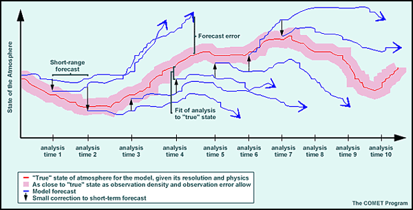
Before each analysis time, the model makes a short-range forecast valid at the time of the analysis. This is the trial field. As the trial field forecast values of the model variables change with time, they may move out of the "zone of truth." The job of the analysis is to use the observed data to bring each variable back into the acceptable range, resulting in an initial analysis which will serve as the basis for the next model forecast.
One major advantage of assimilation cycling is that good information from previous analyses is retained, and so made available for future forecasts. This is particularly important in data-sparse areas. For example, an area in the middle of an ocean may have a couple of ship reports at 12Z which define a low-pressure area. This information is then carried through to 18Z via the trial field. If there are no observations at all in that area at 18Z, the analysis will still "know" about the low at that time because of the assimilation cycling procedure. This means that the analysis is dependent to some degree on the quality of the NWP model used to create the trial field. If the short-range forecast is bad, then the corrections made by the analysis may not be sufficient to bring model variables back into the "zone of truth." This can lead in turn to more bad forecasts.
In summary, the assimilation cycling process is designed to create a four-dimensional representation of the state of the atmosphere in which analyzed values of atmospheric variables are consistent with the physics, dynamics, and numerics of the NWP model used in that process The goal is to extract as much usable information as possible from all the available observations, while avoiding inconsistent information which might corrupt the analysis.
1. The Analysis Should Match Observations » Accountability in Action
Now let's look at an example of how observations are used to correct the trial field in the analysis process. In black are wind barbs of the changes that the analysis made to the trial field 250 hPa winds, as a result of taking into account the available observations.
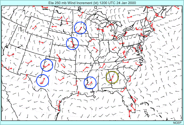
The difference between observed wind and trial field wind can also be calculated. These differences are plotted as red wind barbs at each observing site.
If the analysis were to match perfectly the observations, then the red and black wind barbs would match perfectly. In practice, this rarely happens. Instead, the analysis under-corrects. Changes to the trial field are generally toward the observed wind, both in speed and direction, but are smaller than would be required to match the observations perfectly.
For example, you can see that the wind speed is under-corrected, but the correction is toward the observed value, at stations such as Omaha, Minneapolis, Amarillo, Midland, and Little Rock (blue circles).
Now consider Peach Tree City, near Atlanta (yellow circle), where something unusual happened: the observation shows that the trial field was off by 50 knots. This difference is very large and therefore the analysis assumed the observation was incorrect and so ignored it. As a result, the correction to the trial field shows a light wind in the opposite direction to the observation.
Such a situation is uncommon. If the observation is actually correct, then the analysis will be incorrect, and a forecast bust may occur. In this particular case the NWP models missed a blizzard which occurred after the time of this analysis.
Usually, though, observations are used by the analysis with under-corrections as described earlier. This can have major implications for rapidly-evolving systems, or systems that are entering the radiosonde network for the first time, such as those coming in from the Pacific. The trial field will often underestimate the true intensity of such systems, and so it can take several assimilation cycles before the analysis catches up with their true structure.
1. The Analysis Should Match Observations » Test your Knowledge
Which procedures would be useful to asses the model's initial conditions?
The correct answers are a), c), d) and e)
a) The trial field is an integral part of the analysis, and so weaknesses in the trial field will be reflected in the analysis, especially in data-sparse areas.
b) Many data rejections will indeed be due to incorrect observations. However, it is also possible that correct observations be rejected by the analysis.
c) Patterns in the satellite imagery reflect current atmospheric conditions, and so comparing the imagery to the analysis can help determine whether or not the analysis is on the right track.
d) Assuming correct observations, large differences between the analysis and the observations will indicate areas of the atmosphere whose structure is not well-defined by the analysis.
e) High-resolution numerical models can produce spurious features on a scale smaller than that of the observing network. These features may show up in the analysis through the trial field, and their presence may contaminate the following NWP model forecast.
f) The analysis must retain internal consistency with the physics, dynamics, and numerics of the model used in the assimilation process. Sub-grid scale processes by definition cannot be resolved by the model, so the analysis will generally not carry the details of those processes. Clearly, the forecaster must be aware of such missed details when issuing a short-range forecast.
g) Large differences in observations may be due to one or more erroneous observations. If the observations are correct, then the differences are probably due to measurement of small-scale features not representative of the average of the grid box. In either case, the analysis is produced according to its own rules governing data rejections and the use of the observations and the trial field. While the analysis may have weaknesses in such cases, it may also produce the best possible representation of the atmosphere given the model's own dynamics, physics, and numerics.
1. The Analysis Should Match Observations » Reality
That the analysis should match observations is a misconception.
In summary:
- The initial analysis should not necessarily look exactly like the observations.
- In some cases there are meteorological features that observations can resolve, but that the analysis can't.
- The NWP model provides data for the analysis via the trial field in the assimilation cycling process
- In most cases the analysis under-corrects for discrepancies between the observations and the trial field.
- Observations with large discrepancies are generally ignored. In the rare case in which such observations are actually correct, ignoring them may result in a bad forecast.
These characteristics of the assimilation and analysis processes must be considered by the forecaster in his assessment of numerical model forecast guidance.
To learn more about this topic, visit: Understanding Data Assimilation: How Models Create Their Initial Conditions, a module that is part of the NWP Distance Learning Course.
Understanding Data Assimilation: How Models Create Their Initial Conditions
2. High Resolution Fixes Everything
- Misconception
- Grid and geophysical field resolution can affect the forecast
- When higher resolution helps the QPF
- Do mesoscale models guarantee better forecasts?
- Test Your Knowledge
- Reality
2. High Resolution Fixes Everything » Misconception
In trying to produce the best possible NWP forecast, you might think that the model initial analysis should match exactly the observations used in that analysis, but you would be wrong.
Let's explore what's behind this counter-intuitive misconception.
The initial analysis comes from a complicated combination of the observations and a short range model forecast called the trial field (also referred to as the first guess field), and is designed to provide the best possible starting point for the forecast model. The analysis must account for such factors as differing accuracy of the various observing systems, the possibility of incorrect observations, and the relative importance of the trial field and the observations. The analysis must also be consistent with the model's own resolution and its own physics. For these reasons, the model initial analysis will differ somewhat from the observations.
2. High Resolution Fixes Everything » Grid and geophysical field resolution can affect the forecast
A snow event in southern New England on December 30, 2000, demonstrates that running a higher resolution model doesn't always lead to a better QPF.
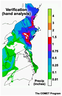
The verification of storm total precipitation shows a region of heavy snow with amounts in the range of one to one-and-a-half inches of liquid equivalent over southern New York and northern New Jersey. There were even some small areas over southern New York where observed maximum snow amounts exceeded 1.5 inches of liquid equivalent.
The AVN model, with a horizontal resolution of 80 kms provided a forecast of amounts in the one to one-and-a-half inches liquid equivalent range, centered on western Long Island. The model had the right idea, but forecast this area a little too far south and east.
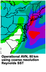
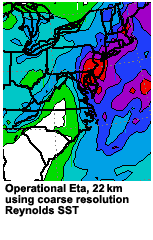
The ETA model, with a 22 km horizontal resolution, placed its area of heaviest precipitation even farther south than the AVN. Comparing the two forecasts with the verification, it is clear that the AVN QPF was better than that of the ETA for this case, despite the fact that the ETA's resolution was almost four times better than the AVN's.
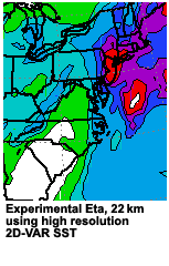
Why did this happen? To answer that, let's take a look at the same event using an experimental ETA run, which incorporates a high-resolution sea surface temperature analysis. We see that the QPF from the experimental run was much improved from the operational ETA QPF.
When using the coarse operational SST analysis, the ETA model did not perform as well as the AVN. The ETA forecast improved only when it used a higher-resolution SST which more closely matched the ETA's grid resolution. The extra information led to a better QPF. The AVN model's resolution better matched that of the coarse SST analysis, and forecasters would have been better off trusting its QPF in this case, despite the operational ETA model's higher resolution.
In summary, in this case higher model resolution did not "buy" a better forecast. Rather, it just increased the ETA model's sensitivity to the sea surface temperature. The higher-resolution SST had a significant positive impact on the ETA model's QPF. The AVN, on the other hand, with its lower resolution, performed reasonably well with the operational coarse SST analysis.
2. High Resolution Fixes Everything » When higher resolution helps the QPF
Now let's take a look at a scenario in which a higher-resolution model does lead to a better precipitation forecast.
Here we are looking at potential flooding in southern California on February 23, 1998, as strong on-shore flow meets a topographical barrier. The observed rainfall was very heavy in parts of Los Angeles, Ventura, and Santa Barbara counties, with amounts exceeding 8, and even 12 inches in places.
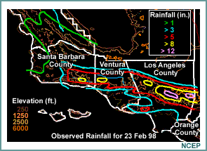
Comparing the QPFs of the 29 km ETA and the 10 km ETA with the observed precipitation amounts, it is easy to see that the higher resolution QPF matches the verification chart more closely.
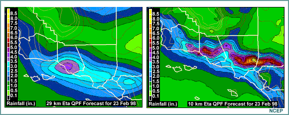
Why is this so? In the previous example we saw that higher resolution did not lead to a better forecast.
The answer lies in the resolution of the topography and the fact that a well-forecast synoptic scale flow is interacting with that topography. This is a a best-case scenario for gaining value with a higher-resolution model. Looking closely at the model topography, shown in thin grey lines on the two forecast charts, you can see that much more detail is visible at 10 kms resolution than at 29 kms.
In both cases the topography is forcing vertical motion and therefore precipitation in the strong southwesterly flow, but the forcing differs according to the detail of the topography. The higher-resolution model does a much better job in locating the areas of heavier precipitation. The amounts are still underforecast—by 4 inches in some cases—but the areas of heavier rainfall closely match the observed pattern. The 10 km resolution forecast is a very useful one.
In this situation we have a strong synoptically-forced flow moving over well-defined topography. Furthermore, there are no significant secondary effects, such as mountain valley circulations or sea breeze circulations.Given these circumstances, higher model resolution can generally be expected to lead to a more accurate forecast of precipitation.
2. High Resolution Fixes Everything » Do mesoscale models guarantee better forecasts?
Modern very high-resolution NWP models with highly sophisticated microphysics are available to the research community. Would the operational use of such models automatically lead to better forecasts?
Let's take a look at an example of this by reviewing a high-resolution post-event model run for a summer severe weather case in which a tornado occurred near Oklahoma City in May, 1999.
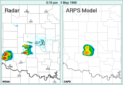
The sequence of images presents the observed radar reflectivities from 5:10 through 8:50 in the evening of May 3, along with model-simulated reflectivies at those times, based on the non-operational ARPS model. This model features 3-km horizontal resolution, accounts for ice microphysics, and includes a variety of other sophisticated components. The model was initialized with radar data after the first convective cells formed earlier in the day.
The model forecast and the observations are similar in terms of the general area in which convection is taking place. However, if we take a closer, frame-by-frame look and focus on county lines, we can see that the model is not accurate in the details of location and intensity of the convection. Such details would be necessary to produce accurate warnings.
For example, at 6:50 a tornado is occurring here near this impressive hook echo while the ARPS model is showing the cell to be weakening and already off to the northeast.
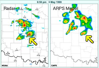
Clearly, high-resolution models such as the ARPS will not always provide better forecasts. One practical reason for this is simply timeliness: output from such models is not available soon enough to be useful in forecasting. For example, in this case the model had to be initialized with radar data from the first developing cells, and its forecast output was available much later than that.
More importantly, we must recognize basic limitations which are inherent in very high-resolution models. Observational data used by such models may not always be available at the required resolution, so the initial analysis may "fill in the holes" with incorrect details. However, a correct convective forecast requires that the model's structure of the atmosphere be "just right". This includes the atmospheric moisture, which is highly variable and notoriously difficult to analyze. Moreover, it's not enough to have perfect upper-atmospheric structure in the model: boundary layer and surface variables and processes, such as temperature, moisture, mixing, vegetation, soil types, and evaporation determine in part the instability and so the convection. These are modelled to a greater or lesser degree, but a given model may not include a full treatment of all these elements. Finally, numerical representations of precipitation processes through model physics packages are unlikely to be perfect. For example, outflow boundaries, which often initiate new convection, may be missed in the model. For these reasons, there is no guarantee that any model, even with very high resolution, will forecast convective precipitation in the right general area, and even if it does, it is unlikely to handle correctly all the details of location and intensity of the convection.
Limitations of High-Resolution Models:
- The analysis may fill in data "holes" with incorrect details.
- Correct forecasts of convection rely on accurate depiction of upper-atmospheric parameters, some of which are highly variable and so difficult to analyze.
- Important boundary-layer and surface variables may not be modeled well.
- Precipitation processes are unlikely to be represented perfectly.
2. High Resolution Fixes Everything » Test your Knowledge
Which of the following statements summarizes a message you should take from the discussion about this misconception?
Discussion:
The correct answers are b) d) and e)
a) A large-scale flow can be well-defined even with low-resolution data. Such a flow can interact with the detailed topography of a mesoscale model to produce more accurate forecasts of wind and precipitation than would be possible with a lower-resolution model.
b) Sharp features in fields such as sea surface temperature or vegetation can affect the forecast at scales which can be handled by higher-resolution models; such sharp features are lost in lower-resolution analyses.
c) If the assimilation is handling smaller-scale features correctly and if the model physics for those scales is adequate, then it is possible that the higher resolution model will produce a better forecast.
d) Terrain has a direct effect on some variables such as precipitation and wind. More-detailed model terrain can clearly interact with the atmospheric flow in certain situations to produce a better forecast.
e) More data means that the analysis takes longer to run. If the horizontal and vertical resolution are increased, then the model time step must be shortened in consequence, and model execution time increases because of the higher resolution in space and time. Finally, higher-resolution output means bigger files, which result in slower dissemination.
2. High Resolution Fixes Everything » Reality
Running models at higher resolution will NOT always lead to more accurate forecasts.
One of the main things to keep in mind is that all components of the model function synergistically. This means that higher resolution works best when the model also includes improved and more realistic physics packages, and more detail in the surface specifications of fields such as soil, vegetation, sea-surface temperature, and topography. High-resolution data must also be available, and the data assimilation system must handle those data correctly at the resolution of the model. In fact, the question of data and data assimilation is probably the biggest factor in obtaining improved forecasts from high-resolution NWP models.
In summary:
- The model should be able to take advantage of surface fields at a resolution comparable
to its grid resolution.
- Realistic physics packages must be incorporated into the model.
- Availability of high-resolution data and correct data assimilation are of highest importance.
To learn more about this topic, visit: Model Fundamentals - version 2 and Operational Models Encyclopedia. Both are modules of the NWP Distance Learning Course.
3. A 20 km Grid Accurately Depicts 40 km Features
- Misconception
- Resolving Small-Scale Features
- Weather Features as Waves
- Larger-Scale Features in Numerical Models
- Understanding Degradation
- Test Your Knowledge
- Reality
3. A 20 km Grid Accurately Depicts 40 km Features » Misconception
With the help of high-resolution models you can improve the odds of making a perfect forecast, even for small-scale features. For example, high-resolution models will help you pinpoint the greatest concentration of lake effect snow, and they will provide an accurate forecast of the effects of downslope winds on regional temperatures. Right?
Not so fast! These ideas stem from a common misconception about NWP forecasts.
In any numerical model, features that span only 2 or 3 grid points are never well resolved. A high-resolution model with a 20 km grid will not resolve a 40 km feature with any accuracy. In fact, it will take a model resolution of less than 10 kms to do an adequate job, and even then it will not be accurately represented for very long into the forecast.
3. A 20 km Grid Accurately Depicts 40 km Features » Resolving Small-Scale Features
Let's look at some typical small-scale features and see how they are resolved by a high resolution model.
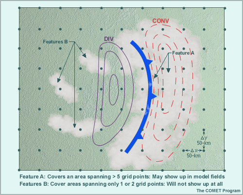
Here is a convergence/divergence couplet associated with a cold front. The grid spacing, ΔX, is 50 kms. The clouds associated with the large region of low-level convergence—feature A—will show up in the model fields. On the other hand, smaller features in the divergence region, such as features B, span less than 4 grid points and will not be properly resolved.
The convergence zone features are carried in the 50 km grid, but this does not mean that they are well resolved, or that their evolution can be accurately forecast. Let's take a look at why even a model with a 20 km model grid would have difficulties with these features.
3. A 20 km Grid Accurately Depicts 40 km Features » Weather Features as Waves
Atmospheric features in numerical models can be represented in wave-form. Here is a simplified 4ΔX representation by a single sine wave of an observed frontal precipitation band associated with a convergence/divergence couplet.
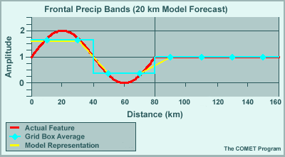
The blue diamonds show each grid box's average value for the feature, and the yellow line shows its resulting representation in the model.
The size of the feature in relation to the grid is 4ΔX. In this example, ΔX equals 20 kms, the resolution of the model in terms of grid-point spacing. The feature is 80 km in length and is represented as a 4ΔX wave.
What we see is that the wave in the model—the yellow line—has roughly only 2/3 the amplitude of the actual wave, as well as a blocky appearance not found in the original feature. The wave is visible, but the details are not well represented.
Problems arise if we use this depiction to make a forecast. Let's put the model in motion and see how its representation of the feature diverges from the actual feature over a short period of time.

During 170 minutes, the observed feature moves one full wavelength. The model's forecast, however, shows substantial phase lag. The model wave becomes broader and loses amplitude. The result is a poor forecast of this particular feature.
3. A 20 km Grid Accurately Depicts 40 km Features » Larger-Scale Features in Numerical Models
How does this compare to the way the model handles a larger scale feature? For instance, one that spans 10 grid points. Let's take a look.

This wave represents a 10ΔX feature, for example a moisture plume spanning 200 km on the same 20 km grid. The model's representation of this feature is far more refined than that of the 4ΔX case.
Putting the model in motion, we see that the 10ΔX wave retains much better definition of this feature's phase and amplitude over the same time period. Overall, the forecast of this feature is much better than that of the 4ΔX wave.
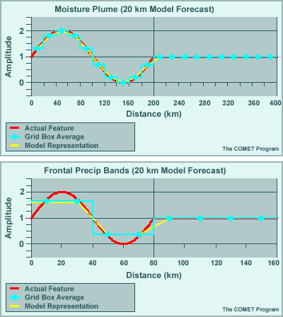
The details of phase lag, wavelength broadening, and amplitude retention differ from model to model, but there are no models that will accurately reproduce a 4ΔX or smaller feature. A 10ΔX feature, however, will be well represented, and even features spanning as few as 6 to 8 grid points will initially be fairly well represented. But, as we will see in the next example, even features of that size will deteriorate over time in the model forecast.
3. A 20 km Grid Accurately Depicts 40 km Features » Understanding Degradation
We can get a better understanding of why the analyses degrades with time by looking at the wave equation used to represent a feature. Here we are looking at a 7ΔX feature, a mesoscale vortex spanning 140 km on a 20 km grid.
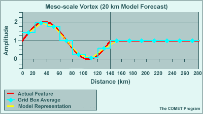
The initial representation compares favorably to the actual feature. After putting it in motion we see that the wave degrades with time. It falls behind the actual feature, loses amplitude, and creates the beginnings of a small trailing wave.

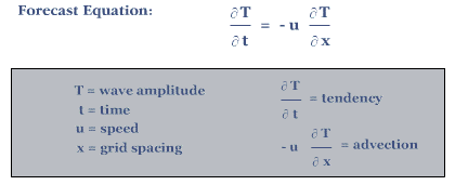
This simple forecast equation shows the relationship between the local rate of change of the variable T and its advection by the wind. From the equation, we see that the advection term contains the gradient of T, which must be accurately represented as a spatial finite difference in the model in order to be well forecast by that model.

If we look at the third grid point, we see that the model gradient—the slope of the green line between the second and fourth grid points—deviates from the actual gradient (blue line) at that point. In fact, the actual gradient, which is the slope of the wave at grid point 3, is steeper.
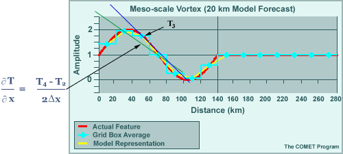
In running the model, the discrepancy between the represented gradient and the true gradient quickly becomes larger and the forecast degrades from reality.
So the more grid points available—the smaller the ΔX—the more closely the model can represent atmospheric features and in turn maintain a more accurate forecast. With a larger ΔX, there are fewer grid points to represent the feature, and as a result the forecast degrades faster.
3. A 20 km Grid Accurately Depicts 40 km Features » Test Your Knowledge
Terminology for these questions:
Resolved means that the feature exists initially in the numerical model at roughly the right scale, location, and amplitude, but not necessarily with enough definition to be accurately forecast by that model. Features as small as about four grid lengths will be resolved in an NWP model. If the feature spans fewer than four grid points, it will be "aliased," which means it will be misinterpreted as having a longer wavelength than it really does.
Well forecast means that the feature is resolved with enough definition in the model's initial analysis that it will be carried forward in time with reasonable accuracy in the subsequent model integration. A feature will be well forecast if it spans at least 8-10 grid points.
Question 1
Suppose you are working with a numerical model that has a 12 km grid.
Question
Would a 500 mb short wave be resolved? Would it be well forecast?
Discussion:
A short wave is a dynamic feature that exists and moves within the atmosphere at various levels. A 500 mb short wave can be thought of in terms of the wave equation that was studied earlier in this session. Typical 500 mb short waves exist on a horizontal scale of hundreds of km, so in a 12 km model they will be more than simply resolved; they will be well forecast.
Question 2
Suppose you are working with a numerical model that has a 12 km grid.
Question
Would a lake breeze on the Lake Superior coast be resolved? Would it be well forecast?
Discussion:
Features such as lake and sea breezes and valley winds have their origins in terrain or in land-sea differences, but also have a dynamic component in the atmosphere once they are set up. A lake breeze on the Lake Superior coast could be quite long along the coast, but its scale perpendicular to the coast might be on the order of tens of km inland, and tens of km offshore. Willet and Sanders (Willet, H. C., and F. Sanders, 1959: Descriptive Meteorology. Academic Press. 355 pp.) state that "by late afternoon, the sea breeze reaches its broadest extent, sometimes extending as much as 30 miles inland and 30 miles out to sea." This horizontal scale of 60 miles, or approximately 100 km, appears to be a maximum for a sea breeze. Assuming a lake breeze with a width of 50 km (spanning about four grid points) at the initial time of the 12 km model, then such a breeze would be resolved (assuming good model definition of the land-sea boundary). This breeze is too small to be well forecast in the model, though. Breezes from smaller lakes, or the initial stirrings of the Lake Superior lake breeze, would have much smaller widths than 50 km. A lake breeze with a width of 20 km at initial analysis time would span less than two grid lengths of the model, and so, while the breeze would likely exist within the model, it would be aliased and incorrectly represented initially. Such a breeze would be neither resolved nor well forecast by the model.
Anecdote
"Some of you might remember the LFM model which was used in the 80s and early 90s. Its horizontal resolution was coarse by today’s standards, with a grid spacing greater than 100 km. This model would at times produce lake breezes for both Lakes Superior and Michigan. These model breezes would then converge over Eau Claire, Wisconsin, and the resulting vertical motion could in turn lead to model forecast precipitation there. This was totally unrealistic; the model did include lake breezes, but was wrong in the details of their sizes and locations. Current higher-resolution models will handle lake breezes better than the LFM, but still can not be counted on to provide correct details of their sizes and locations."
Question 3
Suppose you are working with a numerical model that has a 12 km grid.
Question
Would orographic precipitation related to a strong southwesterly synoptic flow from the Pacific onto the BC coast be well forecast? At what scale?
Discussion:
Orographic precipitation is a feature directly linked to the topography, through its interaction with the prevailing synoptic scale flow. Except for this interaction, there are no atmospheric dynamics that cause the precipitation area to move or intensify. The precipitation will always coincide with the topography. As a result, if the synoptic flow is handled correctly, then the orographic precipitation will be well forecast down to the limit of the model's grid spacing and its topography (12 km resolution). In such cases, the feature need not span 8-10 grid points to be well forecast.
3. A 20 km Grid Accurately Depicts 40 km Features » Reality
To summarize, high resolution models will not resolve small-scale features. Such models must have a resolution that is appropriate for the scale of the features that are to be included in the numerical representation.
The most important factor in how well any atmospheric feature is resolved is its size compared to the model's grid spacing. Features that span less than 8 to10 grid points, although fairly well represented initially, will quickly degrade in any model. Small-scale features, such as sea breezes, lake effect snow, and downslope winds, have no hope of being correctly handled by an NWP model unless they span 8 to 10 grid points. In a high-resolution model with, say a ΔX of 10 km, features must be larger than 80 kms to be well resolved and maintained during the model integration!
In Summary
- A key factor in determining whether a feature can be resolved is the feature size compared to grid spacing.
- Atmospheric features must be at least 8 times larger than the grid spacing (ΔX) in order to be well resolved and sustained for a reasonable forecast length.
To learn more about this topic, visit: Horizontal Resolution, a section of the NWP Distance Learning Course
module: Impact of Model Structure and Dynamics.
4. Surface Conditions Are Accurately Depicted
- Misconception
- Surface Fields in Eta
- Surface Fields in GEM
- Comparison of Surface Fields in Eta and GEM
- Example: Greenness Fraction in Eta
- Vegetation's Impact
- Vegetation Effects in a Single Column Model
- Test Your Knowledge
- Reality
4. Surface Conditions Are Accurately Depicted » Misconception
With today's highly sophisticated NWP systems, one would assume that surface conditions are always correctly represented. For example, the model always knows exactly where snow lies on the ground, and it knows the current state of vegetation. It uses analyzed and accurate values of soil moisture, and defines flooded areas of land when they occur.
Not necessarily. Although modern NWP models do have sophisticated treatment of surface conditions, there are situations in which their forecasts will need significant adjustments due to inaccuracies in the specification of initial surface conditions used in the model, or to weaknesses in how the model handles those surface conditions.
4. Surface Conditions Are Accurately Depicted » Surface Fields in Eta
Let's begin by reviewing how two operational NWP models, the American Eta and the Canadian GEM regional, handle vegetation and soil moisture as of spring, 2002.
We'll start with the Eta model.
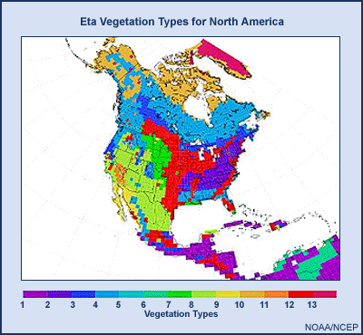
For vegetation type, a one-degree by one-degree global vegetation type climatology is used. The values for each Eta grid box are taken from the nearest one degree by one degree midpoint. The resolution of this vegetation-type dataset is much coarser than the resolution of the Eta model itself. This might lead to model errors in vegetation type. The vegetation fraction (also known as the greenness fraction) is the portion of each model grid box covered by live vegetation. In the Eta, vegetation fraction data are based on a 1985 to 1989 remote sensing dataset of NDVI (Normalized Difference Vegetation Index) with a resolution of 0.144 degrees. The actual vegetation fraction may be ahead of or behind this climatology.
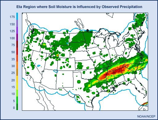
To specify soil moisture, the Eta land surface is coupled to a four-layer soil model. In the Eta's assimilation cycle, starting 12 hours before its initial time, precipitation analyses using radar and rain gauge data over the continental U.S. and over southern Canada near the Canada-U.S. border are used to "nudge" the Eta's forecast precipitation toward the observed values. The resulting precipitation analysis, which is similar to the observed amounts, then feeds the land surface model. The result is that the soil moisture is more or less anchored to the observed precipitation in the area enclosed by the blue line in the chart you see below. Nowhere is an actual soil moisture measurement used. Over the vast majority of Canada as well as Alaska, precipitation used for soil moisture is provided directly by the Eta model without any "nudging" from observations. In these areas, therefore, the soil moisture is anchored to the Eta forecast precipitation.
4. Surface Conditions Are Accurately Depicted » Surface Fields in GEM
Page 3: Surface Fields in GEM
Now we'll look at how vegetation and soil moisture are treated in the GEM regional model, in which a land surface scheme known as ISBA (Interactions among the Soil, Biosphere and Atmosphere) handles surface processes.
The vegetation type used by ISBA over North America comes from a USGS (United States Geological Survey) climatological database on a 1-km by 1-km grid. It includes 24 vegetation types. Vegetation characteristics such as leaf area index, vegetation fraction and root depth change from day to day in the model according to a pre-established table. The vegetation variables are spatially averaged to provide the GEM model with values representative of its grid areas. Since a climatology is used, the actual vegetation conditions may not match those seen by the model.
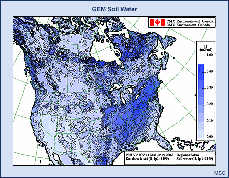
ISBA uses a two-level soil moisture model. Once per day, at 00Z, in a technique known as sequential assimilation, errors in GEM's forecasts of air temperature and relative humidity at the two-meter level (the level of the Stevenson screen) are used through an error-feedback procedure to modify the soil moisture fields on the model grid. No actual soil humidity measurements are used in this process.
Both the GEM regional model and the Eta model calculate evaporation and evapotranspiration from the surface as a function of their soil moisture and vegetation characteristics.
4. Surface Conditions Are Accurately Depicted » Comparison of Surface Fields in Eta and GEM
Eta
vegetation
For vegetation, a one-degree by one-degree global vegetation type climatology is used. The values for each Eta grid box are taken from the nearest one-by-one degree midpoint. The resolution of this vegetation-type dataset is much coarser than the resolution of the Eta model itself. This might lead to model errors in vegetation type. The vegetation fraction (also known as the greenness fraction) is the portion of each model grid box covered by live vegetation. In the Eta, vegetation fraction data are based on a 1985 to 1989 remote sensing data set of NDVI (Normalized Difference Vegetation Index) with a resolution of 0.144 degrees. The actual vegetation fraction may be ahead of or behind this climatology.
soil moisture
To specify soil moisture, the Eta land surface is coupled to a four layer soil model. In the Eta's assimilation cycle, starting 12 hours before its initial time, precipitation analyses using radar and rain gauge data over the continental U.S. and over southern Canada near the Canada-U.S. border are used to "nudge" the Eta's forecast precipitation toward the observed values. The resulting precipitation analysis, which is similar to the observed amounts, then feeds the land surface model. The result is that the long-term soil moisture is more or less anchored to the observed precipitation over the continental U.S. and extreme southern Canada. Nowhere is an actual soil moisture measurement used. Over the vast majority of Canada as well as Alaska, the precipitation that feeds the land surface model is provided directly by the Eta model without any "nudging" from observations. In these areas, the long-term soil moisture is anchored to the Eta forecast precipitation.
snow
Snow cover and snow depth for the Eta come from a daily 23-km resolution NESDIS snow cover analysis merged with the daily 47-km resolution AFWA snow depth analysis valid at 18Z. Both are based on satellite observations, and synoptic snow depth data are also used in the AFWA analysis. The AFWA analysis is quality-controlled against the NESDIS snow cover observations for approximately the 18-22Z period, to create a 1/2-degree by 1/2-degree daily snow depth analysis valid at 18Z. This analysis is first used in the 06Z Eta model run, and then in subsequent 12Z, 18Z, and 00Z runs. The snow analysis is therefore 30 hours old by the time it is used in the 00Z Eta run. Snow depth is a dynamic variable in the Eta and can change during the model integration.
ice
The ice coverage analysis in the Eta is based solely on satellite data. It comes from the SAB (Satellite Analysis Branch) and is updated once per day, valid at 00Z, on a 25.4-km resolution polar stereographic grid true at 60 degrees North. This analysis includes data for the Great Lakes. No information on ice thickness is included.
SST
Sea surface temperatures are analyzed on a one-half-degree by one-half-degree grid, using the most recent 24 hours of buoy and ship data as well as satellite-derived temperatures. The 2D-VAR technique used by this analysis has a correlation length such that detail in the SSTs tends to be preserved. This analysis is updated once per day, in time for the 00Z run of the Eta model.
GEM
vegetation
In the GEM regional model, a land surface scheme known as ISBA (Interactions among the Soil, Biosphere and Atmosphere) handles surface processes.The vegetation type used by ISBA over North America comes from a USGS (United States Geological Survey) climatological database on a 1-km by 1-km grid. It includes 24 vegetation types. Vegetation characteristics such as leaf area index, vegetation fraction, and root depth change from day to day in the model according to a pre-established table. The vegetation variables are spatially averaged to provide the GEM model with values representative of its grid areas. Since a climatology is used, the actual vegetation conditions may not match those seen by the model.
soil moisture
ISBA uses a two-level soil moisture model. In a technique known as sequential assimilation, errors in GEM's forecasts of air temperature and relative humidity at the two-metre level (the level of the Stevenson screen) are used through an error-feedback procedure to modify the soil moisture fields on the model grid once per day, at 00Z. This is done over all of North America. No actual soil humidity measurements are used in this process.
snow
The Canadian Meteorological Centre snow depth analysis is driven by precipitation and temperature forecasts from the GEM global model, and incorporates all available snow depth observations. This global analysis is updated every 6 hours, on a 1/3-degree by 1/3-degree latitude-longitude grid. The analysis is interpolated to the model grid to provide its initial snow conditions, which are never more than 6 hours old for any model run. Snow depth is a dynamic variable in GEM regional, and can change during the model integration.
ice
The Canadian Meteorological Centre ice coverage analysis uses SSMI satellite data along with daily ice observations from the Canadian Ice Service. This global analysis is updated once per day on a 1/3-by 1/3-degree Gaussian grid, and incorporates all ice data received during the 24 hour period ending at 00Z. Ice cover observations for 118 selected Canadian lakes from the Canadian Ice Service are also used, but are available only once per week. No ice thickness information is included in this analysis.
SST
The sea surface temperature at the Canadian Meteorological Centre is analyzed on a global latitude-longitude grid with a resolution of 37 km. The analysis is updated once per day, at 00Z, and incorporates data over the previous 24 hours from satellites, ships, and buoys. In the absence of observations, the SST analysis slowly reverts to climatology. This poses no particular problem over the oceans, but may lead to large errors over Canadian lakes in the absence of lake temperature observations. Except over the Great Lakes, such observations are scarce.
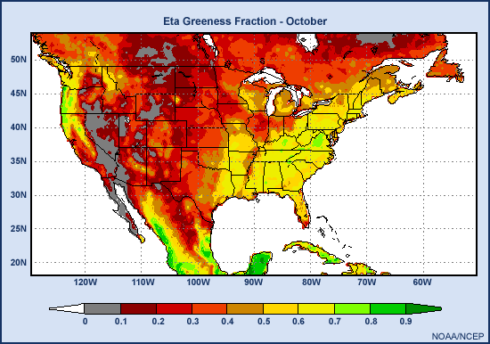
4. Surface Conditions Are Accurately Depicted » Example: Greenness Fraction in Eta
How can surface fields impact model forecasts? As an example, let's consider how the Eta model accounts for the vegetation or greenness fraction.
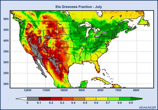
Take a look at this series of images depicting the vegetation fraction across the US, southern Canada, and parts of Mexico and the Caribbean. Specifically, let's zero in on some details in two highly cultivated regions: the Kansas-Oklahoma winter wheat belt and the midwestern corn belt .
In January, much of the area inland and north of 35 degrees is barren except for the winter wheat belt where the winter wheat crop was planted in the late fall.
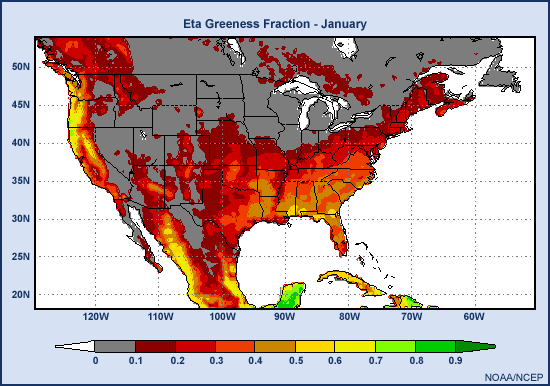
By April, the wheat belt reaches its peak greenness while most other areas are just beginning to green up. The corn belt is an exception: it remains relatively brown compared to the neighboring areas. These other areas are covered with deciduous trees.
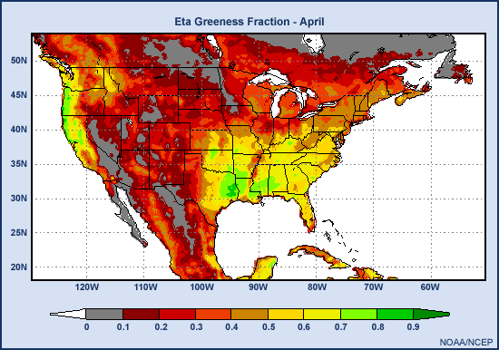
Moving into the summer months, the winter wheat is harvested, leading to a brown down in that area while the forested regions of the central and eastern U.S. reach peak greenness. The corn belt then remains relatively brown until July when there is a sudden explosion of vegetation as the corn grows and ripens.
In the fall the corn is harvested and browns down by October. Meanwhile the forest begins to brown down as well while the winter wheat is planted for next year's harvest and the cycle begins again.
The impact of these seasonal changes in the vegetation greenness fraction can be significant. Next we'll take a look at how theses changes impact the models.
4. Surface Conditions Are Accurately Depicted » Vegetation's Impact
Why do we care about the amount of green vegetation in a numerical weather prediction model? Because it has a significant impact on low level fluxes of sensible and latent heat, which in turn determine low-level atmospheric temperature and humidity.
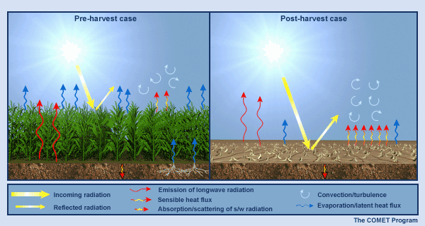
Green vegetation impacts humidity levels by controlling the amount of evaporation that takes place. It extracts water from sub-surface soil layers, and that water in turn can be transpired during the day into the atmosphere.
Vegetation also impacts surface energy levels. With vegetation present, energy that would otherwise go directly into heating the surface instead goes into evapotranspiration with profound impacts on surface temperature and humidity, and on the planetary boundary layer's temperature, humidity, and static stability.
4. Surface Conditions Are Accurately Depicted » Vegetation Effects in a Single Column Model
To illustrate vegetation's impact on surface temperature, we have taken what is known as a single column model to represent a single grid box and have run two cases for a full diurnal cycle. Single column models are often used to validate the physical parameterizations in NWP models.
In this example, the forcing for each case is identical and comes from observed data from an atmospheric cloud and radiation test bed in the southern Great Plains in June, 1997. The physical parameterization considered is the one used in both the AVN and MRF models. The only difference between the two cases is the amount of vegetation in the grid box. In what we will call a pre-harvest case, the grid box is 90% covered by cultivated vegetation while in the post-harvest case, only 20% of the grid box has green vegetation. The resulting diurnal cycles for surface and near-surface temperatures are shown.
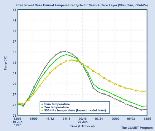
Above is the diurnal cycle for the pre-harvest case. Predicted skin temperature is in gray, 2 meter diagnosed temperature in green, and 995-mb predicted temperature in yellow. Below is the same variables for the post-harvest case are shown.
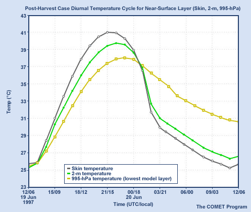
There is a clear difference in the diurnal cycles between the two cases. The temperatures after harvest are 5 to 6 degrees Celsius higher than pre-harvest temperatures. Differences in moisture and characteristics of the planetary boundary layer, while not shown here, are similarly significant.
Since convection is generally parameterized in NWP models using planetary boundary layer or surface parcel stability parameters, it follows that errors in the model vegetation fraction could result in errors in convective initiation.
It is important for the regional forecaster to know if the actual state of vegetation matches the model's current greenness fraction.. Depending on how closely they match, the model output may or may not need significant adjustments for use in weather forecasts.
4. Surface Conditions Are Accurately Depicted » Test Your Knowledge
Question 1
Question
Fields and forests have greened up much earlier than usual in your forecast area due to very warm and moist spring conditions. How might that affect your prediction of surface parameters for an upcoming warm sector convective situation?
Maximum surface temperature:
The correct answer is d)
In this case, the model has significantly less vegetation than is actually present. As a result, model maximum temperatures will be too warm by several degrees C, as a large portion of the incoming solar radiation in the model will be used to heat the surface rather than for evapotranspiration through the vegetation canopy.
Question 2
Question
Fields and forests have greened up much earlier than usual in your forecast area due to very warm and moist spring conditions. How might that affect your prediction of surface parameters for an upcoming warm sector convective situation?
Boundary layer depth:
The correct answer is b)
Because of the cooler land surface resulting from increased evaporation, the PBL depth will be less than forecast by the model.
Question 3
Question
Fields and forests have greened up much earlier than usual in your forecast area due to very warm and moist spring conditions. How might that affect your prediction of surface parameters for an upcoming warm sector convective situation?
Near-surface winds and turbulence:
The correct answer is b)
The cooler land surface results in less turbulent mixing in the PBL, which in turn reduces downward momentum transfer from levels above the surface where the winds are stronger, so that the surface winds are weaker in this case.
Question 4
Question
Fields and forests have greened up much earlier than usual in your forecast area due to very warm and moist spring conditions. How might that affect your prediction of surface parameters for an upcoming warm sector convective situation?
Relative humidity:
The correct answer is b)
More evapotranspiration from plants means more humidity near the surface and within the PBL. Therefore, model RH is too low in the PBL. Because of weaker turbulence in the PBL due to the cooler surface temperatures, humidity is not mixed upward as far as in the warmer case when few plants are present. This means that the actual RH near and above the top of the PBL will be lower than forecast by the model in this situation.
Question 5
Question
Fields and forests have greened up much earlier than usual in your forecast area due to very warm and moist spring conditions. How might that affect your prediction of surface parameters for an upcoming warm sector convective situation?
In this situation should the probability of convective precipitation:
The correct answer is c)
With full vegetation, low level temperatures will be lower than forecast by the model, but low level humidities will be higher. In terms of convective available potential energy, the two effects act in opposite directions, so the net effect is not clear a priori. What the forecaster can do is to create a modified forecast sounding based on his best estimate of expected low-level temperature and dewpoint, and from this sounding judge the convective potential of the situation.
Question 6
Question
Suppose the ground is bare at 00Z over southern Saskatchewan, but heavy snow falls and is observed to cover the ground at several observing stations in the 01Z to 05Z period. Which is the earliest subsequent run for each of these models that "sees" this new snow?
The Canadian snow depth analysis is updated once every 6 hours. The 18Z analysis is completed before the 00Z model run, and is used in that run. Similarly, the 06Z analysis is used in the 12Z model run. The GEMs are never more than 6 hours behind on the snow depth they "see" at their initial times of 12Z or 00Z. The snow analysis used by the Eta is updated once per day, based on 18Z USAF snow depth data, and quality-controlled by the 18-22Z NESDIS snow cover observations. It is "seen" for the first time by the next 06Z Eta run. This means that for the 00Z Eta run, the snowfall analysis used approaches 30 hours old. Snow in the 01-05Z period will not be "seen" by the Eta until the following 06Z run, over 24 hours later.
Question 7
Question
In which of the models, GEM regional; GEM global; and Eta, is the snow depth a dynamic variable (one that changes with time) during the course of the model integration?
The correct answer is d)
This is an example of the fact that surface processes can be handled differently by different models within their integrations. As of spring, 2002, GEM regional and the Eta both have dynamic snow depths. GEM global, on the other hand, "sees" the initial snow analysis but keeps it constant through its entire integration. This will change in the future when the ISBA system is connected to GEM global.
4. Surface Conditions Are Accurately Depicted » Reality
To summarize, initial surface conditions are not necessarily accurately represented in each model run. This can be due to the use of climatological surface fields as well as factors such as timing, technique, resolution, data availability, and quality control schemes of the routines used to analyze the surface fields.
In addition to potential analysis problems, you need to remember that surface processes are approximated rather than precisely modeled. They can also be highly interdependent. Furthermore, different numerical models not only can use different initial analyses of surface fields, but usually will handle those surface fields differently within their integrations. These facts guarantee that the question of surface fields and processes in NWP models is a highly complicated one.
In general, a forecaster must know how surface field data are collected and incorporated into the NWP models in order to understand how the surface fields may be deviating from reality. This understanding helps to better evaluate the model output and adjust the forecast.
In reality, the latest surface conditions for an NWP model may:
- be based on climatology;
- not match the model grid scale;
- not make it into the current model run;
- not be accurately analyzed;
- not be well-handled within the model integration.
To learn more about the treatment and effects of the various surface fields, see the COMET Web module entitled, Influence of Model Physics on NWP Forecasts (https://www.meted.ucar.edu/nwp/model_physics/navmenu.php?tab=1&page=3-0-0&type=flash)
In addition to the surface field descriptions listed in this page, current information about these and many other model characteristics can also be found in the Operational Models Encyclopedia (https://www.meted.ucar.edu/training_module.php?id=1186) on the MetEd Website.
5. CP SCHEMES 1: Convective Precipitation is Directly Parameterized
- Misconception
- Convection: Sequence of Events in Nature
- Convection: Sequence of Events in a Model with No Convective Parameterization
- Adjustment Schemes
- Mass-Flux Schemes
- Compensating for Shortcomings of Convective Parameterization Schemes
- Test Your Knowledge
- Reality
5. CP SCHEMES 1: Convective Precipitation is Directly Parameterized » Misconception
Predicting convection and resulting precipitation is an integral part of many forecasts. So you would think that the primary purpose of an NWP model's convective parameterization scheme is to predict convective precipitation.
In reality, precipitation is a by-product of a model's convective parameterization scheme. The real purpose of such a scheme is to release instability so that the models don't predict convection on the grid scale. We wouldn't want the 80km grid AVN producing an 80km wide convective updraft, for example - this would be completely unrealistic.
5. CP SCHEMES 1: Convective Precipitation is Directly Parameterized » Convection: Sequence of Events in Nature
Of course NWP models must account for convection in some manner.
To do so they use parameterizations that attempt to reproduce the natural life cycle of a convective event. What might happen in a model that uses no convective parameterization? To answer this question, let's compare a natural convective sequence with the sequence that would occur in a model with no convective parameterization.
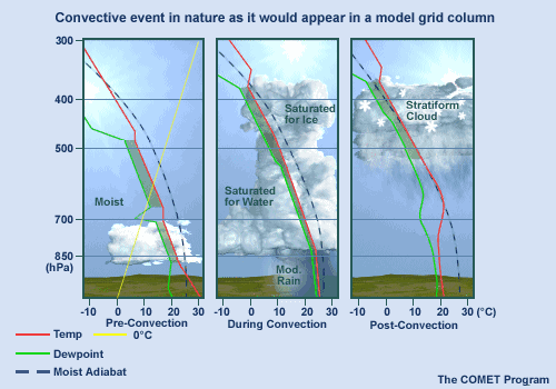
First, let's look at the life cycle of a typical convective event in nature as it would appear within a model grid column.
We begin with an unstable sounding favorable for convection. A strong updraft, which occurs in only a small portion of the grid column, quickly transports heat and moisture to the upper troposphere as the cloud builds. Compensating, weaker subsidence outside the updraft--yet still within the grid column--also occurs. Rain falls within a small portion of the grid area, while the rest of the grid area remains precipitation-free. After the convection weakens, rain from stratiform cloud at middle and upper levels may fall. The final result is a stable post-convective atmosphere.
5. CP SCHEMES 1: Convective Precipitation is Directly Parameterized » Convection: Sequence of Events in a Model with No Convective Parameterization
Now, let's examine how a model with no convective parameterization handles the same event.
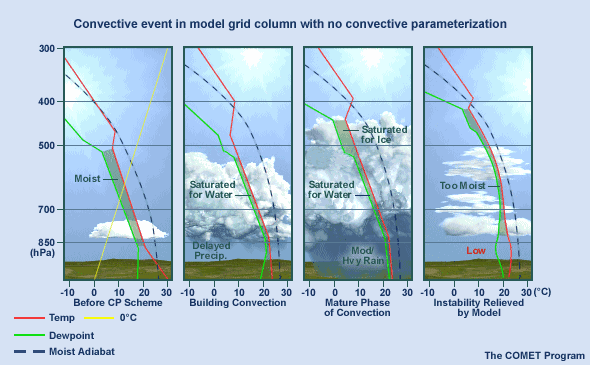
Beginning with the same unstable sounding, the model builds convection using grid-scale vertical velocities. These are very small compared to real convective updrafts--on the order of centimetres per second--so the cloud grows slowly.
One result of this slow buildup is a delay in precipitation onset compared to the natural event. In addition, as things progress, the model creates heavy precipitation across the entire grid box, and the cloud does not extend as high as it would in nature. Also, the whole grid column becomes completely saturated through the depth of the model cloud.
This leads to the release of a large amount of latent heat in the lower and middle troposphere in the mature phase of the convective cloud, which in turn can cause a low pressure centre at the surface.
In the model's post-convective phase, the surface low pressure centre remains and much of the sounding is nearly saturated. These conditions can easily lead to more model precipitation.
Clearly, a model that executes with no convective parameterization scheme has no hope of producing a good precipitation forecast. Worse yet, it can even create an over-developed frontal wave or a surface low-pressure centre that is too deep. NWP models must use convective parameterization schemes if they are to have any hope of avoiding these problems.
5. CP SCHEMES 1: Convective Precipitation is Directly Parameterized » Adjustment Schemes
In essence, convective parameterization schemes rearrange heat and moisture to counteract the models' tendencies to create grid-scale convection.
There are two major types of convective parameterizations: adjustment schemes and mass-flux schemes. Let's compare the two, starting with an example of an adjustment scheme.
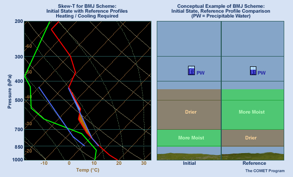
The Betts-Miller-Janjic (BMJ) adjustment scheme shown here is used in the operational Eta model. In this scheme, model soundings of both temperature and humidity are forced toward reference soundings, which are represented in the skew-T diagram by the blue curves. In an unstable atmosphere such as we have here, the adjustment process causes upward movement of moisture and a reduction in precipitable water. The precipitable water removed from the column must then fall as model precipitation.
This adjustment scheme is fairly crude and has several limitations. First, the reference profiles are fixed, and will usually miss the details of any given situation. Second, the scheme is triggered only for soundings with deep moisture. Third, when triggered, the scheme often precipitates too much, leaving too little humidity for precipitation occurring later or downstream. Fourth, the scheme does not account for capping inversions act to inhibit convection. Finally, it does not directly account for any changes below cloud base.
5. CP SCHEMES 1: Convective Precipitation is Directly Parameterized » Mass-Flux Schemes
Most of today's models use mass-flux schemes, which form the second main class of convective parameterizations. GEM regional uses the Fritsch-Chappell mass flux scheme, but this will change in fall, 2002 with the introduction of the Kain-Fritsch mass-flux scheme. The RUC and AVN models also use the Kain-Fritsch scheme.
Mass-flux schemes are designed to stabilize an atmospheric column by reducing the amount of CAPE (Convective Available Potential Energy). The process is depicted in this schematic. Air enters the sub-grid scale updrafts and is rapidly transported to middle and upper levels of the troposphere. At the same time there is compensating subsidence in the environment outside the updrafts, and there are also convective downdrafts.

As air rises in the sub grid-scale updrafts, humidity is removed and then falls as precipitation. Some of this precipitation is evaporated in the downdrafts, which leads to cooling. Entrainment and detrainment also occur. The amount of air processed, which in turn determines the amount of precipitation, is based on the amount of stabilization needed.
The environmental subsidence tends to warm the column at mid and upper levels, while the convective downdraft tends to cool the lower levels. This leads to a more stable model atmosphere, but without the formation of grid-scale convection.
Mass flux schemes are considered to be more realistic than adjustment schemes. Their QPFs can look disorganized due to their triggering of convection in scattered grid boxes. While probably more realistic, such patterns can make model evaluation more difficult. One notable limitation of the Kain-Fritsch scheme is its tendency to develop unrealistically deep saturated layers in active convective areas, so that post-convective stratiform precipitation in those areas may be overforecast.
5. CP SCHEMES 1: Convective Precipitation is Directly Parameterized » Compensating for Shortcomings of Convective Parameterization Schemes
Convective parameterization schemes in general have limitations. Different schemes can have very different effects on model soundings, with more or less realism, and those effects are advected downstream. The timing and placement of convection depend on the model's large-scale forcing, its boundary layer forcing and details of the scheme's triggering process, such as the minimum convective cloud depth in mass-flux schemes. Model winds may be indirectly affected by a convective parameterization scheme, but are not directly changed by model convection as real winds are by real convection.
Given the shortcomings of convective parameterization schemes, you cannot rely on the model's convective QPF for precipitation amounts or even convective timing and location. You can evaluate the model's large scale forcing, instability and moisture, and adjust them as necessary to define potential convective areas. Your knowledge of smaller-scale effects, such as boundary layer details, can be used to refine the forecast. Remember that convection in a given region of the model causes significant changes to its atmosphere in that region and downstream--just as real convection does in the real atmosphere--but the model changes may be very different from the actual changes in nature. Such model changes can therefore reduce the usefulness of model diagnostics such as frontogenesis and PV. However, your knowledge of the limitations and biases of the convective parameterization scheme you are working with may help you to further refine the forecast.
5. CP SCHEMES 1: Convective Precipitation is Directly Parameterized » Test Your Knowledge
Question 1
Question
Which of the following statements about CP schemes in general are true?
The correct answers are a), c), and e)
CP schemes were designed to release instability, not to forecast convective precipitation. Condensation and precipitation are created as by-products of the schemes' acting to remove the instability.
Most schemes do not directly modify the horizontal wind field.
Real convective cells have significant updrafts and downdrafts, but CP schemes do not directly alter the vertical motion field. However, future very high-resolution non-hydrostatic models with explicit convection (and so no need for a CP scheme) will be able to directly modify both the horizontal and vertical motion fields.
Question 2
Question
Which of the following statements about particular CP schemes are true?
The correct answers are c) and e)
The BMJ technique uses reference profiles, and one of its limitations is that it does not account for the inhibiting effect of capping inversions. The Kain-Fritsch scheme is a mass-flux scheme in which stabilization of the atmospheric column is achieved through reduction of CAPE. Among its advantages are the facts that this scheme accounts for capping inversions, and also it includes downdrafts with associated cooling near the surface.
5. CP SCHEMES 1: Convective Precipitation is Directly Parameterized » Reality
To summarize, the primary purpose of convective parameterization schemes is not simply to predict convective precipitation.Rather, it is to release instability so that the models don't produce grid-scale convection and its associated adverse impacts.
Convective precipitation is a necessary by-product of these schemes. For this and other reasons, convective precipitation is notoriously difficult for numerical models to predict. In general, the forecaster cannot rely on the model's convective QPF for precipitation amounts or even location and timing of convection. Modifications to the model's forecast are often necessary.
Reality:
- Convective parameterization schemes are designed to release model instability.
- Convective precipitation is a necessary by-product of the convective parameterization.
- The forecaster often must make significant changes to the model's convective QPF.
To learn more about this topic, visit: Convective Parameterization a unit in the module: How Models Produce Precipitation and Clouds, part of the NWP Distance Learning Course.
Also, don't miss CP Schemes 2: A Good Synoptic Forecast Implies a Good Convecective Forecast, one of the other misconceptions in this series.
CP Schemes 2: A Good Synoptic Forecast Implies a Good Convecective Forecast
6. CP SCHEMES 2: A Good Synoptic Forecast Implies a Good Convective Forecast
- Misconception
- Model Grid Scale vs Reality
- Fine Tuning CP Schemes
- Overactive CP Schemes
- Underactive CP Schemes
- Different Schemes in the Same Model
- Test Your Knowledge
- Reality
6. CP SCHEMES 2: A Good Synoptic Forecast Implies a Good Convective Forecast » Misconception
Suppose an NWP model has a good synoptic forecast, with accurate large-scale forcing and pre-convective soundings. It follows that convection and all its effects will also be adequately forecast.
Not at all.
Even if the model is performing well at the synoptic scale, it will not necessarily do a good job on weather elements influenced by convection such as precipitation, temperature, humidity, wind, and pressure. There are a variety of reasons for this. Let’s explore some of them.
6. CP SCHEMES 2: A Good Synoptic Forecast Implies a Good Convective Forecast » Model Grid Scale vs Reality
One key reason is that the convective parameterization schemes of current operational NWP models work at the scale of the model grid, while convection in nature occurs at much smaller scales. In effect, the model’s convective parameterization scheme must “invent” information at these smaller scales. A related problem is that the initial analyses used by the models can miss existing atmospheric details important for convection, due to the fine scale of those details.

Consider a model with a 15-km grid spacing. Each 15 x 15 km grid box holds only one value per layer for temperature, humidity, and winds, while convection in the atmosphere occurs at much smaller scales. So the model would really need many more small grid boxes to have any chance of depicting convection at the proper scale.
For example, in some situations boundary layer rolls are a critical element in convective initiation. A 1-km grid model can resolve such features and thus can initiate the associated convection.
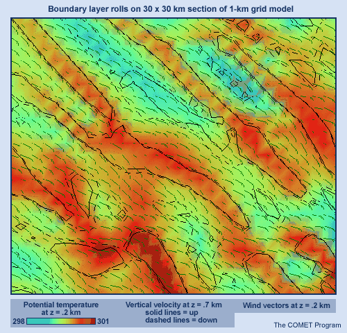
While there is no guarantee that all the forecast details of this convection will be correct in the 1-km model, clearly a 30-km model or even a 15-km model has no chance whatsoever of resolving the physical processes involved in creating such convection. This point is illustrated schematically in the graphic.
6. CP SCHEMES 2: A Good Synoptic Forecast Implies a Good Convective Forecast » Fine Tuning CP Schemes
Another complicating factor in modeling convection and its effects is the difficulty in adjusting convective parameterization schemes to work as well as possible within the model for all weather situations. These schemes try to model atmospheric processes and use parameters related to these processes that can be adjusted, or tuned. Typically, sensitivity experiments are conducted and the parameters are tuned to give what is considered the “best” result over a variety of cases. Compromises are inevitable, though, and the chosen tuning will not be the best for every situation.
To illustrate this point, let’s consider some results from the GEM regional model with a 16-km grid and the Fritsch-Chappell convective parameterization. We’ll look at forecast precipitation in the 12-36 hour period from two model runs initialized at 1200 UTC on 4 August 1998.
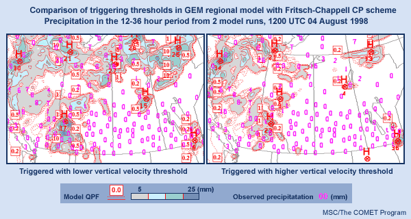
The only difference between the two runs is in the tuning of the Fritsch-Chappell scheme.
In these images, the numbers in magenta are the observed precipitation in mm at various locations. The model QPF is represented by thin dashed or solid red contours, with values of 0.2, 0.5, 1, 5, 10, and 25 mm. Amounts above 5 mm are emphasized through shading in three different colors. The small boxes are labels for some of the QPF contours.
In the first run, the scheme’s trigger function was programmed with a less selective value: the threshold vertical velocity at cloud base was relatively low. In the second run, a more selective value, with a higher threshold vertical velocity, was used.
The differences are striking. The first run generally has more precipitation over a wider area than the second, which is expected since the scheme was able to convect more easily in the first case. Neither result is perfect. For example, observed precipitation amounts of 7, 15, 3, and 2 mm over northeastern Alberta and northern Saskatchewan were missed by the second run. Even though the first run did over-forecast amounts in this area, it provided a better “signal” for what happened there. On the other hand, in other areas such as southeastern BC, the first run was clearly too generous with its precipitation, while the second run was somewhat better with lower forecast amounts. But note that exactly the opposite was true over southeastern Manitoba. There is no single ideal solution, but one single value of the threshold vertical velocity must be chosen for the scheme when it is implemented in an operational model.
6. CP SCHEMES 2: A Good Synoptic Forecast Implies a Good Convective Forecast » Overactive CP Schemes
Another potential problem is that in some situations the model can incorrectly forecast convection because its convective parameterization scheme is either under- or overactive.
This graphic represents what happens if the scheme is overactive, which means that it has an excessive response to some model forcing.
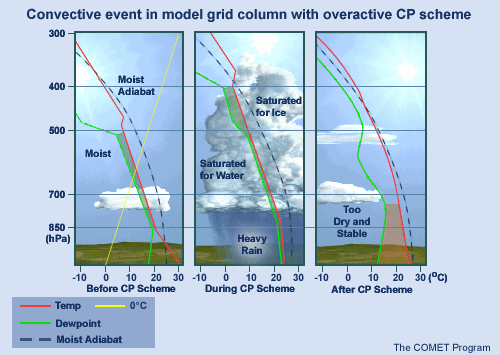
In such cases precipitation is over-forecast in the convective area, but under-forecast downstream. Also, there is too much drying and stabilization in the model soundings both in the convective area and downstream. There are no clear rules for identifying such situations. If the model is forecasting precipitation where it is not occurring, and if most of this precipitation comes from the convective rather than the explicit scheme, then one might suspect an overactive scheme if the model has relatively small pre-convective CAPE values. Recall that the explicit scheme is the parameterization used to forecast precipitation that occurs at scales resolved by the model.
6. CP SCHEMES 2: A Good Synoptic Forecast Implies a Good Convective Forecast » Underactive CP Schemes
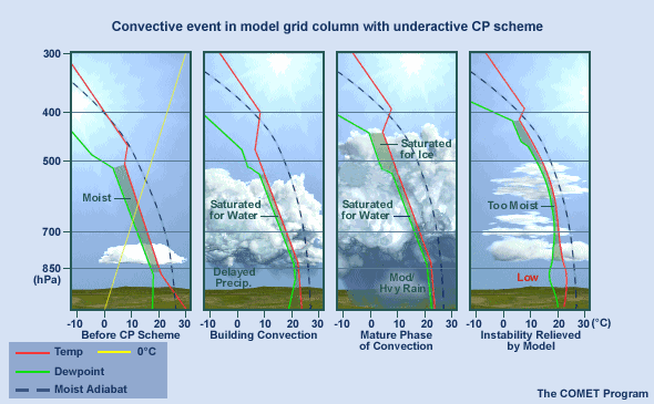
If the convective scheme is underactive but there is sufficient humidity and large-scale lift, then the explicit precipitation scheme takes over and produces excessive precipitation from a model convective cell the size of a full grid box. This is similar to what happens in the complete absence of a convective parameterization scheme, and its effects are most serious for models with grid spacing greater than about 10 km. The result is too much model precipitation, sometimes significantly so, but with delayed onset of precipitation.
There will be too little drying and stabilization in the model soundings, both in the convective area and downstream. Worse yet, this situation can in turn lead to false low-level cyclogenesis, which then feeds back through excess lift and condensation so that the explicit precipitation scheme can then produce even more precipitation. Although this is commonly referred to as "convective feedback," these forecast errors created by convection the size of the entire grid box actually result from what the convective parameterization scheme did not do. At times it can be identified by the presence in the forecast of a sharp precipitation maximum, a small but intense vorticity maximum at 500hPa, and a marked maximum in upward motion at mid levels, all stacked above a surface low. In convective feedback situations, such lows are generally forecast too deep and too far left of the correct track.
6. CP SCHEMES 2: A Good Synoptic Forecast Implies a Good Convective Forecast » Different Schemes in the Same Model
Finally, let’s look at an example of two different convective parameterizations running in the same numerical model. Here too, there can be significant differences in the model forecasts.
We’ll consider two runs of the Eta model from 16 March 2000. The first run was done with the Betts-Miller-Janjic (BMJ) scheme, while the second one used the Kain-Fritsch (KF) scheme. There were no other differences between the two runs.
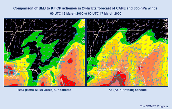
Let’s compare the 24-hour forecasts of CAPE and 850hPa winds from the two runs. Clearly there are significant differences in CAPE over southeastern U.S. There are some interesting differences in the winds as well. Over Georgia, for example, they are generally stronger with a larger southerly component in the Kain-Fritsch run. These differences are due only to the differences between the two parameterizations.
The two runs produced rather different QPFs as well.
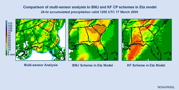
The Kain-Fritsch run emphasized rain over the Gulf of Mexico and southern Alabama much more than the BMJ run , while the BMJ run had more rain over eastern Georgia and much of South Carolina. Comparison with the observed precipitation chart shows that both models had shortcomings in their QPFs.
A detailed look at model soundings from the two runs would shed more light on the specific differences in behavior of the two schemes.
6. CP SCHEMES 2: A Good Synoptic Forecast Implies a Good Convective Forecast » Test Your Knowledge
Question 1
Question
What clues from the model output might indicate that it is exhibiting
"convective feedback"
effects (as a result of grid-scale
convection) at a particular location?
The correct answers are a) and d)
With model convection comes precipitation and a saturated, moist adiabatic atmospheric column. However, if there is too much condensation and too much latent heat release in the model, then a significant upward vertical motion maximum occurs in the column, which causes a surface low pressure centre and a vorticity maximum at 500mb. If all these factors are present and aligned more or less vertically, then the forecaster should suspect the possibility of convective feedback.
Question 2
Question
You suspect that your NWP model's CP scheme is overactive in a convective system that will soon affect your area of responsibility. What effect might this have on the following weather elements?
If very little actual convection is occurring in an area but the model predicted a significant convective precipitation component at that time or location, you might suspect that the CP scheme is overactive there. Model clues as outlined in question 3 should also be considered. An overactive convective scheme may influence your forecast as follows.
a & b) The CP scheme will probably remove too much instability as it overprecipitates. Removing too much instability and moisture from the model atmosphere where convective precipitation is predicted results in air that is too stable and too dry, both in the convective area and, by advection, downstream.
c) The duration of convective precipitation will be too short. The model convective area generates too much rain initially, which then dies out too quickly as the model atmosphere is stabilized too quickly.
d) The subsequent amount of cloudiness will be too little. Excessive drying created by the overactive scheme may lead to an underforecast of subsequent low and middle cloudiness in the model. This will also cause model temperature forecast errors.
e) It is important to remember that these effects can also impact model forecasts at a later time downstream, even after the model's overprediction of precipitation has ended. For example, in this case the model will probably underforecast both precipitation and cloudiness downstream of the main convective area.
Question 3
Question
You suspect that "convective feedback" is occurring in the GEM
regional model in a
forecast valid at 00Z. This involves a
precipitation bull's-eye of 50mm or so in a 6-hour period, and a surface
low-pressure centre forecast in the same location as the precip max. As
a result of the suspected grid-scale convection, you expect that the
model will forecast the low center to be too deep in the following 12
hours. What is/are the most likely model forecast error(s) in
positioning for that low during that time period?
The correct answer is c)
While not true in all cases, what is often noted in such situations is that the NWP models forecast the surface low not only too deep, but also too far left of the correct track. This is similar to the behaviour of any low that is forecast to be too deep: it tends to build its leading ridge too much through warm advection, which in turn deflects the low to the left of the actual track.
6. CP SCHEMES 2: A Good Synoptic Forecast Implies a Good Convective Forecast » Reality
Convection in the real atmosphere affects weather elements such as precipitation, wind, temperature, humidity, and even pressure, both in the convective area and downstream from it. The same is true of model convection. NWP models are often very reasonable in their forecasts of the large-scale, synoptic flow pattern and associated weather elements, but for a variety of reasons this skill does not necessarily transfer down to smaller convective scales in the models. Convective parameterization schemes do attempt to compensate for the lack of resolution of convective events at the sub-grid scale, but with varying degrees of success; different schemes can lead to different results. Another problem is that the model may not be able to resolve data appropriate to convective scales in its initial analysis, while the larger synoptic scale is easily resolved. Furthermore, as we have seen, no single tuning of a convective parameterization scheme will work well in all situations. Moreover, in some cases the scheme may be overactive or underactive. An underactive scheme can lead to convective feedback, in which even the MSL pressure can be badly forecast.
These model problems can occur in model convective areas, even if the synoptic flow is well forecast there. The result in those areas is inaccurate model forecasts of fields influenced by the convection, such as precipitation, temperature, humidity, wind, and pressure. Worse yet, such model inaccuracies can propagate to affect other regions downstream of the original convective areas.
Reality
- NWP models work on grid scale – convection in nature occurs at smaller scales
- The CP scheme tuning does not work well for all situations
- In some situations, CP schemes may be over- or underactive
- Different CP schemes lead to different results
To learn more about this topic, visit: Convective Parameterization a unit in the module: How Models Produce Precipitation and Clouds, part of the NWP Distance Learning Course.
Also, don't miss CP Schemes 1: Convective Precipitation is Directly Parameterized, one of the other misconceptions in this series.
CP Schemes 1: Convective Precipitation is Directly Parameterized
7. Radiation Effect are Well-handed in the Absence of Clouds
- Misconception
- The complexity of radiative processes
- Example of the effects of clouds
- Example of clear sky solar insolation bias
- Example of clear sky skin temperature bias
- How models address radiation processes
- Test Your Knowledge
- Reality
7. Radiation Effect are Well-handed in the Absence of Clouds » Misconception
The only problem with representing radiation in NWP models results from difficulties in emulating the effect of clouds.
Not so.
Certainly clouds complicate the radiation picture, but the truth is that shortwave and longwave radiation are highly complex phenomena to represent, even under clear skies. A full treatment would require intensive schemes that would monopolize computer-processing cycles. The simplifications necessary to streamline the calculations only add to the problem of predicting the effects of solar and infrared radiation in the Earth-atmosphere system. Some variables such as air temperature, skin temperature of the model surface, and evaporation are highly dependent on radiative effects. These variables are in turn related to others such as instability and convective precipitation. The forecast for all these variables depends in part on a correct forecast of radiation and its effects.
7. Radiation Effect are Well-handed in the Absence of Clouds » The complexity of radiative processes

On average, about half of all incoming solar radiation reaches the surface. The other half is reflected, scattered or absorbed by clouds, various atmospheric gases, and other constituents. In addition, the earth’s surface has varied characteristics influencing the amount of solar radiation absorbed and reflected, and itself emits longwave radiation. This longwave radiation is in turn transmitted through the atmosphere, or absorbed and re-emitted by clouds and various atmospheric gases.
All in all, this complex balance of radiative absorption, reflection, scattering, and emission is very difficult to represent in an NWP model. The effect of clouds is only one part of this complex interaction.
7. Radiation Effect are Well-handed in the Absence of Clouds » Example of the effects of clouds
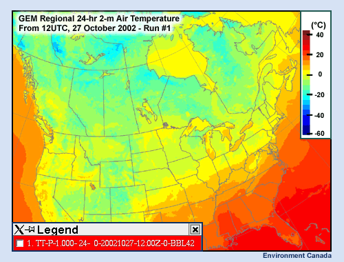
Let’s start by considering a case in which radiative effects did interact with model clouds. This will give us an idea of the complexity of the problem in general, and of errors that can be caused by radiative problems in NWP models. A clear-sky radiative case will follow.
In the fall of 2002, it was noticed that an experimental version of the Canadian GEM regional model was having some trouble with forecast air temperatures close to the model surface: they were often significantly too cold.
Let’s look at two 24-hour forecasts of air temperature at 2 m above the model surface from an initial time of 12Z October 27, 2002. In these graphics, reds represent warmer temperatures and blues cooler temperatures.
Why is the second forecast showing warmer air temperatures than the first? What modification was made for the second run? The answer involves how ice crystal clouds are parameterized in the model. This parameterization defines the effective radius and concentration of ice crystals that make up cold clouds as a function only of the model’s ice water content. In the first run, the model “saw” fewer but larger ice crystals in its ice clouds. In the second (below), it “saw” more but smaller ice crystals in those clouds. This difference resulted in different air temperatures in the two runs.
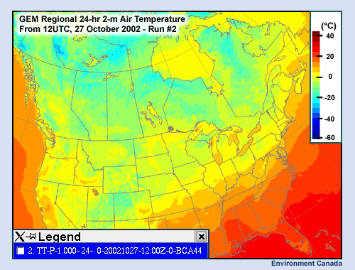
The interaction between the model’s longwave radiation and its ice crystal clouds was important for the air temperature in this example. In the second run, it appears that the larger concentration of smaller crystals in the ice clouds acted to more efficiently absorb longwave radiation emitted by the earth, and then re-radiate it back downward. The extra downward longwave radiation acted to increase the forecast air temperature.
How big was the effect? We can see the answer in the graphic below, which shows the temperature difference between the two runs. Over most of North America, the first run was between zero and 5ºC colder, as indicated by the light green shading. Over parts of northern Quebec, northwestern Ontario, and the western U.S., the light blue shading shows even larger differences in the range of 5 to 10º. These are significant differences, caused by what might at first seem to be a relatively minor change in the model’s cloud parameterization.
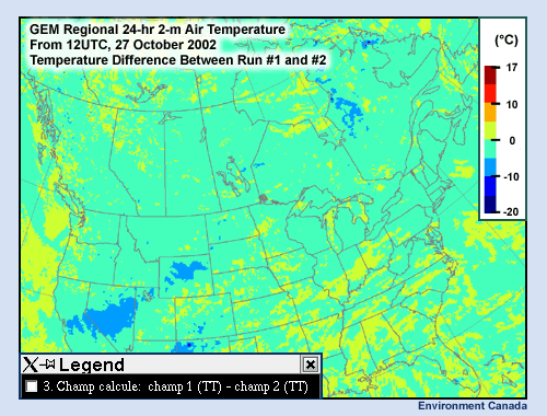
The modified model of the second run produced warmer temperatures and verified much better for this case, as well as others. The modification was subsequently added to the experimental model to improve its temperature forecasts.
7. Radiation Effect are Well-handed in the Absence of Clouds » Example of clear sky solar insolation bias
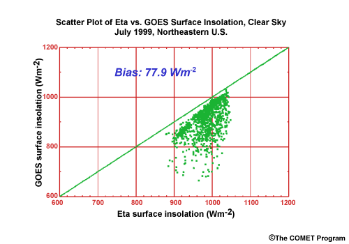
What if there are no clouds? It turns out that even on clear-sky days, numerical models can have a hard time making accurate temperature predications due to problems in modeling radiation processes.
Here is an example of a solar radiation problem in a set of clear-sky cases over the northeastern U.S. in the operational Eta model from July 1999.
Depicted in this scatter plot are the GOES-measured surface insolation versus the Eta-predicted insolation, in watts per square metre. The line representing a perfect, no-bias forecast runs diagonally from the lower left to the upper right corner of the graphic.
All data points to the right of the no-bias line indicate model surface insolation that is greater than the observed insolation. Some of those points show a positive model error of as much as 300 watts per square meter. The mean bias is approximately 78 watts per square meter. It has been calculated that this equates to a positive model skin temperature bias of approximately 6ºC.
7. Radiation Effect are Well-handed in the Absence of Clouds » Example of clear sky skin temperature bias
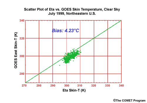
In this graphic is the same set of clear-sky cases, but with measured versus predicted skin temperature in degrees Kelvin. Once again, the diagonal line represents the ideal case of no bias.
Here the data points have an overall positive bias of 4.2ºC in the Eta’s predicted skin temperature, as compared to the measured GOES temperatures. This is not quite the previously calculated bias of 6º, based on the surface insolation data, but is still a significant positive bias.
Clearly, the Eta has radiative problems under clear model skies, but this is only part of the story. It turns out that complex, often non-linear interactions among components of an NWP model can lead to unexpected effects, such as offsetting errors. In fact, the Eta model’s surface physics package does have errors that partially offset its positive solar radiation bias. These errors in may be related to too much ground heat flux or too much evaporation for a given soil moisture condition. The existence of such offsetting errors means that eventual improvements to the surface physics package may actually result in an increased positive bias in the model’s near-surface temperatures!
7. Radiation Effect are Well-handed in the Absence of Clouds » How models address radiation processes
In general, how do models address radiation processes? They do so in various ways:
-
By breaking the atmosphere into layers and predicting or diagnosing the amount of cloud, absorbing gas and aerosols in each layer
-
By using layer-mean values of variables with which radiation interacts, and layer-mean calculations of the effects of both shortwave and longwave radiation
-
By taking into account the radiative effects of each layer on each adjacent layer
-
By making simplifying assumptions about cloud presence, type, and structure, and
-
By calculating radiative effects at the surface, and the resulting influence on the atmosphere in the planetary boundary layer
The largest errors in radiation calculations do result from cloud effects. However, as we have seen, significant model errors related to radiative effects can also occur under clear skies.
One final point to note is that in order to save computing time, radiation schemes are not called as frequently as the model’s dynamic time-step. In the Eta, for instance, they are called every 60 minutes, while the dynamics are calculated every 90 seconds. This procedure can increase inaccuracies in the model’s radiation calculations.
7. Radiation Effect are Well-handed in the Absence of Clouds » Test Your Knowledge
Question 1
Question
Suppose you are working with a model that is known to have a warm bias in its forecast surface temperatures due to solar radiative effects. It is the night shift on a summer night, and you expect a sunny morning with convective clouds developing in the afternoon. What modifications will you have to make to the afternoon values of the following atmospheric variables?
Since the model max temperature is too high, then its PL will be too deep, and as a result it will forecast too much mixing with too much turbulence. This means that winds that are too strong will be mixed down to the surface by the model. Therefore, the forecaster must reduce the forecast depth of the PBL, and must also reduce the near-ground winds and turbulence.
In the actual atmosphere, there will be less evapo-transpiration than in the model due to the lower surface temperatures. This would seem to imply a lower RH near the ground in the real atmosphere. However, there will also be less mixing in the actual atmosphere due to its lower PBL. This means that dry air from the free atmosphere above the PBL will not be able to mix down as much as model forecasts. The near-ground temperature is also lower than forecast by the model, so that the actual atmosphere will end up with a higher RH at the ground. B the same reasoning, the more vigorous vertical development of the model PBL will result in too much upward mixing of near-surface moisture to the top of its PBL.
Even though the RH near the ground is somewhat higher than the forecast by the model, the specific humidity tends to be less because of the reduced evapo-transpiration, resulting in less latent energy available for convection. Combined with cooler actual near-surface temperatures, actual instability will be less in the real atmosphere than in the model, and it is likely that any convective precipitation generated by the model will be overdone.
Question 2
Question
Suppose you are working in the cold season with a model that has a known cold bias in its forecast near-surface temperatures due to infrared radiative effects. What is the most likely effect on model precipitation overall in this situation?
The correct answer is Model precipitation type too “cold”
Since the bias affects the temperatures near the ground, there is no obvious link between the model precipitation amounts and the bias. Cold-season precipitation often has its origins at the middle levels due to the dynamics of synoptic weather systems. On the other hand, a cold low-level temperature bias could affect the forecast precipitation type. In a situation of rain versus freezing rain, the freezing rain could be forecast over too large an area. Similarly, in a situation of snow versus freezing rain, the snow could be forecast over too large an area.
7. Radiation Effect are Well-handed in the Absence of Clouds » Reality
To summarize, the absorption, reflection, scattering, and emission of shortwave and longwave radiation are complex processes that are difficult to represent in an NWP model. The effects of clouds are only one element of this complexity. Models can have radiative problems under clear skies as well. The story is complicated even more by the presence of possible offsetting errors in NWP models: fixing problems in one model physical process may expose weaknesses in others.
Awareness of the biases and limitations of a model’s radiation scheme can certainly help the forecaster to correct a model forecast in some situations.
To learn more about this topic, visit: Atmospheric Processes, a section of the "Influence of Model Physics on NWP Forecasts" module of the NWP Distance Learning Course.
8. NWP Models Directly Forecast Near-Surface Variables
- Misconception
- Illustration of the 2-m Temperature Calculation in GFS Model
- Diagnosis Technique in the GEM, Eta, and RUC Models
- Potential Problems
- Model Vertical Coordinate and Interpolation Distance
- Terrain Representation in the Models
- Test Your Knowledge
- Reality
8. NWP Models Directly Forecast Near-Surface Variables » Misconception
The near-surface temperature, humidity, and wind obtained from NWP models come from direct model forecasts of those variables.
Of course, the dynamics of NWP models are calculated at all levels of the model grid, but that is only part of the story. The model physics must also come into play, not only at upper levels, but also at the lower boundary surface. The surface physics package, through its calculation of skin temperature, for example, necessarily has a major effect on the near-surface air temperature. Dynamics alone cannot account for how the model surface, or skin, affects the near-surface temperature, humidity, and wind. Rather, values of these variables obtained from the model dynamics must be “merged” in some fashion with those obtained from the surface physics. This process is often referred to as the “diagnosis” of near-surface variables. In this sense, the model does generate the values of those variables, but it does not directly forecast them on its grid.
8. NWP Models Directly Forecast Near-Surface Variables » Illustration of the 2-m Temperature Calculation in GFS Model

This graphic depicts schematically how the GFS model creates its 2-m temperature field in each grid box. The lowest-layer midpoint temperature represents the average temperature for the lowest atmospheric layer of the model. The skin temperature comes from the model’s surface energy balance. Both are used to interpolate to a 2-m temperature value.
In the GFS, a logarithmic weighting is used for the interpolation to account for the fact that the greatest rate of change of temperature with height occurs very close to the ground. The blue curve represents such a profile, while the green line shows a linear profile for comparison.
8. NWP Models Directly Forecast Near-Surface Variables » Diagnosis Technique in the GEM, Eta, and RUC Models
The Canadian GEM models use a different approach to calculate the near-surface variables. Monin-Obukhov similarity theory is used to calculate the vertical fluxes of heat, moisture, and momentum at the surface, along with the profiles of temperature, humidity, and horizontal wind between the surface and the first model level above the surface. The treatment is more general than what is done in the GFS and does not assume any particular weighting (such as logarithmic). The GEM technique is designed to provide consistency between the surface layer and the rest of the boundary layer and is valid in both stable and unstable cases and for either strong or light winds. The GEM calculation supplies temperatures and dewpoint depressions at the 1.5-m level and winds at the 10-m level.
The Eta and RUC approach is similar to that of the Canadian models, except for a slightly different diagnosis level for temperature and humidity: 2-m instead of 1.5-m.
8. NWP Models Directly Forecast Near-Surface Variables » Potential Problems
What potential problems can crop up in the model diagnosis of near-surface atmospheric variables?
One is that the diagnosis scheme may lead to poor results if the function used doesn’t accurately represent the variation with height of the variable in question. This is of greater concern in models that use assumed logarithmic profiles, such as the GFS. As we have seen, the GEM, RUC, and Eta models contain more realistic treatments. However, even in these models there is still a functional form assumed through the Monin-Obukhov theory that may not be appropriate in every situation.
Another possible problem that can affect all models is related to the performance of their surface physics packages. For example, the temperature diagnosis relies on the model skin temperature, which comes from the surface physics package via its energy balance. Problems in the physics package can lead to incorrect skin temperatures.
A third source of error is related to model resolution: unresolved terrain and other unresolved surface features down to the microscale will have effects on near-surface temperature, humidity, and wind that the model has no hope of defining.
8. NWP Models Directly Forecast Near-Surface Variables » Model Vertical Coordinate and Interpolation Distance
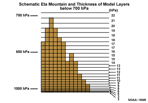
Another factor to consider is the distance over which one is applying the interpolation technique to diagnose the values of near-surface variables. Here we show the model layers for the 50-layer Eta model at surface pressures from MSL to about 700 hPa.
Note that the model layer thickness becomes much larger as the elevation increases. Near MSL, the lowest Eta layer is only about 2.7 hPa thick, while at the 700 level it is 22 hPa thick! This means that at higher levels the Eta interpolation is done through much deeper layers, which can result in greater errors.
The 60-layer Eta model implemented late in 2001 is slightly better because of its somewhat increased vertical resolution.
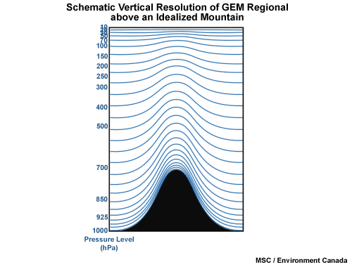
Models that use a terrain-following vertical coordinate do not behave in the same manner. For example, this graphic schematically shows the 28 vertical levels of the GEM regional model above a mountain whose summit is near 700 hPa. The vertical levels above the mountain top are squeezed into less vertical distance than the same levels above MSL, so that the layer thickness decreases as elevation increases. This is the opposite behavior to that of the Eta.
In fact, one can easily calculate that the GEM regional bottom layer is about 5 hPa thick near MSL, and about 3.5 hPa thick at the 700-hPa level. The layer thicknesses for the GFS also decrease with height, but its layers are thinner because of its greater vertical resolution. (GFS uses 64 layers through the first 84 hours of its forecast.) The RUC model vertical coordinate is also terrain-following in the lowest model levels, with a lowest-layer midpoint of only 5 metres above the surface. This smaller interpolation distance will often be to the RUC’s advantage. The Eta, due to its particular vertical coordinates, actually has poorer vertical resolution than the GFS, for example, at levels above 970 hPa.
8. NWP Models Directly Forecast Near-Surface Variables » Terrain Representation in the Models
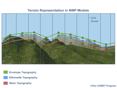
Finally, the effect of model terrain representation on near-surface variables cannot be neglected. This graphic represents a vertical slice through a mountainous region, with various model topographies superimposed. The vertical lines separate the grid boxes, and the dots represent the model terrain height for each grid box. Suppose you must predict the 2-m temperature for a town in the valley near the centre of the image. Clearly, the town’s real altitude is very different from the model’s terrain height at that location. In such a case, the model’s 2-m temperature is of little or no use unless we know both the lapse rate and the difference in elevation between the model topography and the real topography.

What are typical differences in height between model and real terrain? To get an idea, let’s look at a cross section of the GEM regional model terrain along the line shown. This line crosses British Columbia near both Vancouver and Kelowna. Here is the terrain cross section, with approximate pressure levels for reference. Kelowna is located in the Okanagan valley of BC at an altitude of 430 m, but the model terrain places the town near 1120 m, a difference of roughly 700 m! Nor is the effect limited to mountain valleys. Vancouver airport is at about 5 m above MSL, but the model terrain is not steep enough to match the real world at the coast. The model places Vancouver at approximately 110 m, roughly 100 m too high. It is interesting to note that the RUC model attempts to compensate for the terrain representation problem for temperature by extrapolating its temperature downward from the model terrain level to the actual station level, using the lapse rate in the lowest 25 hPa of the model atmosphere.
8. NWP Models Directly Forecast Near-Surface Variables » Test Your Knowledge
Question 1
Question
Mount Washington is the highest point in New England, with an altitude of 1910 m. It is an unusual site because a weather observatory is located at the summit.
What difference would you expect between the altitude of the real observatory and the altitude of the model observatory?
The correct answer is c)
NWP models have smoother terrain than the real world. As a result, stations in valleys are too high in NWP models. This is the usual case since communities and observing sites are almost always located in the valleys of mountainous regions. Conversely, real mountain peaks will be higher than seen by the model.
Question 2
Question
What typical error in the model’s 2-m temperature forecast would you expect for the Mount Washington observatory?
The correct answer is a)
Under usual atmospheric conditions, the temperature decreases with height. Since the model sees the Mount Washington summit at too low an altitude, it will generally forecast the temperature there to be too warm.
Question 3
Question
You expect clear nighttime conditions under a strong high pressure centre with calm winds and significant outgoing longwave radiation.. This should lead to an unusually sharp inversion very close to the ground by 12 UTC. If you believe that the surface physics packages of the GEM regional, GFS, RUC, and Eta are performing equivalently, which model would you expect to have the most difficulty in forecasting the 2-m temperature?
The correct answer is b)
Under these circumstances, the logarithmic profile of the GFS is less likely to correctly handle the sharp variation of temperature with height than the more general formulations of the other models.
8. NWP Models Directly Forecast Near-Surface Variables » Reality
It seems at first glance that NWP models might directly forecast the values of near-surface atmospheric variables. However, the truth is that the results of the model dynamics and the surface physics package must be combined to diagnose the near-surface temperature, humidity, and wind.
Different models do this in different fashions. The GFS uses an interpolation based on a logarithmic profile, while the GEM, Eta, and RUC models use more general formulations involving Monin-Obukhov similarity theory as the basis of their diagnosis.
Potential errors can come from several different sources:
1. The procedure used may not accurately reflect the vertical profile;
2. There may be errors in fields such as skin temperature in the surface physics package;
3. The effects of unresolved terrain and other unresolved surface features can not be accounted for;
4. Relatively large interpolation distances can result in greater errors; and
5. Model terrain representation in the mountains can cause problems because of inaccurate model terrain height.
If the forecaster recognizes the presence of such errors in NWP models, then he or she may be able to compensate for them in the forecast.
To learn more about this topic, visit the NWP module, Impact of Model Structure and Dynamics, a part of the NWP Distance Learning Course.
9. MOS Forecasts Improve with Model Improvements
- Misconception
- A Brief Introduction to MOS
- An Example of the Development of a MOS Scheme
- Cases with Few Observations of the Predictand
- Smoothing in MOS Schemes
- Advantages of MOS Schemes
- Disadvantages of MOS Schemes/li>
- The Canadian Meteorological Centre’s Updateable MOS Scheme
- In What Situations Might MOS Produce a Poor Forecast?
- Test Your Knowledge
- Reality
9. MOS Forecasts Improve with Model Improvements » Misconception
When an NWP model is improved, its Model Output Statistics forecasts will automatically improve as a result.
Not true. MOS systems are based on statistical relationships between a numerical model’s forecast fields and the observed weather. If the model is changed, then those relationships will also change, and new MOS equations will be required. If the equations are not re-derived, there is no guarantee that the existing ones will provide improved forecasts following the model improvement.
9. MOS Forecasts Improve with Model Improvements » A Brief Introduction to MOS
MOS finds the best statistical relationships between various model forecast variables and the weather elements of interest. If multiple linear regression is used to develop the statistical model, then by its design the model minimizes the root mean square error. Of course, scatter, or variance, is inherent in any statistical relationship. Therefore MOS by its design will produce a few bad forecasts, but will also minimize the frequency and severity of those busts.

Statistical methods work well in situations that are close to “normal.” For example, statistics will always assume that the circulation is from west to east in the mid-latitudes. But it can happen that the actual circulation is significantly different from the one seen on average in the development sample. In using MOS, the forecaster—with his or her human intelligence—must always be on the lookout for abnormal situations in which MOS output must be adjusted or perhaps ignored completely.
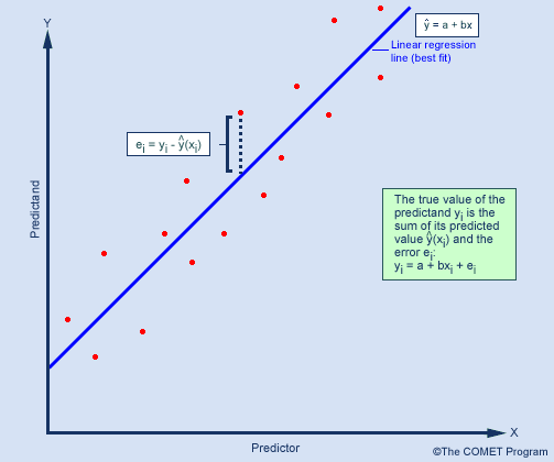
9. MOS Forecasts Improve with Model Improvements » An Example of the Development of a MOS Scheme
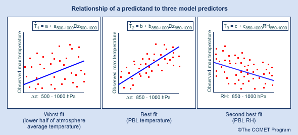
These plots illustrate hypothetical but physically realistic relationships between the maximum 2-m temperature (the predictand) at a given location and several model predictors at that location. The graphics show the relationship of the predictand to the 1000-500 hPa thickness, the 1000-850 thickness, and the 1000-850 mean RH. These three variables represent, respectively, the temperature of the lower half of the atmosphere, the temperature of the PBL, and a surrogate for PBL cloudiness.
In the 1000-500 thickness plot, there is large scatter with a relatively weak positive correlation. In the next plot, though, we see a significant positive correlation between the 1000-850 thickness and the predictand. In the RH plot, the correlation is negative, with relatively wide scatter. In this example, the MOS equations would first make use of the 1000-850 hPa thickness as a predictor of the maximum 2-m temperature, since the correlation is strongest in that case. More predictors would then be added to the prediction equation until the MOS forecast would no longer be significantly improved by further additions.
9. MOS Forecasts Improve with Model Improvements » Cases with Few Observations of the Predictand
In creating MOS relationships, enough data must be available in the development sample to ensure a robust, stable, and statistically significant result. However, some forecast variables such as fog, thunderstorms, and freezing rain occur relatively infrequently. To compensate for this lack of data, climatologically-similar areas can be grouped together to create a larger sample for the development of MOS equations. These regions will vary by season as climatologically-similar regions shift with the seasonal cycle.
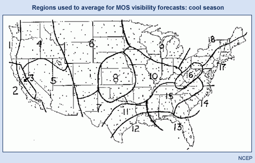
In this graphic, we see 18 cold-season regions grouped together for the development of MOS visibility equations over the continental USA. Those of you familiar with fog climatology will recognize, for example, the foggy Central Valley of California that has been made into a single climatological region.
In the warm season, the regions naturally shift to account for changes in climatological similarities. The entire west coast, for example, is now broken up into two regions, one southward and the other northward from Cape Mendocino. Here the marine influence and cold upwelling water off the coast frequently cause fog. A similar region appears along the New England coast. In addition, the influence of mountainous regions on radiation fog formation can be seen in the central and southern Appalachians.
9. MOS Forecasts Improve with Model Improvements » Smoothing in MOS Schemes
Some MOS schemes apply smoothing to the model fields used as predictor variables. This is done in order to avoid noise and emphasize the synoptic scale signal. These schemes are, in effect, designed not to “see” smaller-scale features predicted by the models. For example, the GFS MOS uses a 25-point (5x5) smoother on a 95-km grid.
In the Canadian MOS system, no such generalized smoothing is done. Instead, the necessary interpolations to station locations are in most cases done directly from the model grid. This retains the full model horizontal resolution (24-km for the GEM regional model as of June, 2003).
However, some predictors involving gradients or Laplacians are calculated on a standard 50-km resolution grid in the Canadian system. This procedure does in effect provide some smoothing for those predictors.
As of June, 2003, tests are underway at the Canadian Meteorological Centre to assess the value of smoothing all predictors before developing the statistical model.
9. MOS Forecasts Improve with Model Improvements » Advantages of MOS Schemes
MOS schemes in general have several advantages.
One is that they account for persistent model biases by using model output variables as predictors. However, this does not mean that they will remove a regime-dependent or situation-dependent bias.
A second advantage is that MOS equations can take advantage of useful model-derived variables that are not directly observed, such as vorticity or vertical velocity.
Also, since they relate model forecast variables to observations, MOS systems can be used to evaluate a model’s performance in its forecast of those variables.
Finally, we note that MOS tends to ensure the reliability of the statistical forecast, but often at the expense of sharpness.
9. MOS Forecasts Improve with Model Improvements » Disadvantages of MOS Schemes
There are also some disadvantages of MOS schemes.
As already mentioned, a change in the driving model means that the MOS equations must be re-derived using data from that new model.
In general, the more cases that go into the statistical relationship, the more reliable it is likely to be. One estimate from a 1986 paper by G. M. Carter is that about two seasons of data (around 300 cases) are necessary for stable statistical relationships to be developed. This means that with traditional MOS development methods, it would take about two years after a model change to develop acceptable MOS equations using predictors from the new model.
Another point to note is that a MOS system is generally expensive to develop and maintain because it may consist of thousands of equations, these being developed for multiple locations according to both valid time and projection time. Given the frequency of model changes in Canada and the USA in the 1990s, it has been very difficult and expensive to maintain statistically-stable MOS systems.
Finally, as already mentioned, while MOS tends to ensure forecast reliability, it does so at the expense of forecast sharpness.
9. MOS Forecasts Improve with Model Improvements » The Canadian Meteorological Centre’s Updateable MOS Scheme
In the 1990s, the Canadian Meteorological Centre investigated an updating method for its MOS scheme: new information about model variables would be ingested into the forecast equations on an ongoing, regular basis. This research led to the Updateable MOS scheme (known as UMOS) that was implemented operationally in the spring of 2001. In it, MOS forecast equations based on output from the GEM regional model are updated four times per month. This means that the current weather regime is taken into account in the development of the UMOS equations. This is true whether the regime is a normal one, or an abnormal one such a prolonged dry period or a prolonged cold spell.
Furthermore, UMOS ensures a smooth transition from old equations to new ones after a significant model change. It does this through a weighting scheme that gives priority to the latest data from the new version of the model. At the same time, it retains enough data from the previous version to ensure the generation of stable statistical relationships.
The Canadian UMOS system is built around two seasons and two transition periods:
- Warm season (16 May - 14 October)
- Fall transition (15 October - 28 November)
- Cold season (29 November - 31 March)
- Spring transition (1 April - 15 May)
A weighting scheme is also used to ensure smooth transition of the MOS equations from one season to the other. The system is designed so that if the GEM model changes near the beginning of the warm or cold seasons, then the blending of old and new equations takes place such that the new model data will have a significant effect on the UMOS forecasts by about one month after the new model implementation. If the model changes near the end of the warm or cold seasons, then the new model data will significantly affect the UMOS forecasts by about three months after its implementation, since in such cases it is also necessary to work through the transition periods to move from the equations of one season to those of the other. However, it is important to note that after a model change it can take up to 300 days for data from the old model to disappear completely from the UMOS system. These times are a vast improvement over the two-year period typically required to develop statistically significant MOS equations through the traditional approach.
9. MOS Forecasts Improve with Model Improvements » In What Situations Might MOS Produce a Poor Forecast?
Statistical schemes have difficulties in unusual events because such events cannot be well represented in the development sample. In general, MOS forecasts will be poor if the statistical relationship is not appropriate for today’s weather. This can happen in several ways:
1. After a model change - As already mentioned, in the traditional approach it can take two years after a model change to develop a statistically-significant set of new equations. The old equations can give poor results during that period. The Canadian UMOS system goes a long way toward eliminating this problem, with new MOS equations able to take full effect within one to three months of a model change.
2. If today’s regime was uncommon or not sampled at all during the MOS development period - It can happen that the current weather regime was not well-sampled, or perhaps was not sampled at all during the MOS equation development period. One example would be if the equations were developed during a couple of relatively mild winters over eastern North America, and then applied in the cold winter of 2002-2003. In the Canadian UMOS system, this is much less of a concern, since the equations are updated four times per month, so that they will reflect an unusual regime if it lasts longs enough.
3. If the particular circumstances of today’s case differ from the norm for similar cases - Such events can happen. For example, a given location that usually has snow cover with an Arctic outbreak could experience one in which there is no snow cover. A traditional MOS system will not handle such an event, since any Arctic outbreaks in its development sample likely included snow cover. The Canadian UMOS system is also unlikely to handle it in the very short term, but will tend to “catch up” if the event lasts long enough to be incorporated into the next few updates of the UMOS forecast equations.
4. If the weather depends on mesoscale effects either not represented by the model, or filtered out of the model data that were used to develop the MOS equations
9. MOS Forecasts Improve with Model Improvements » Test Your Knowledge
Question 1
Question
The GFS MOS was developed using observations and forecasts during the 1997-1998 El Niño and subsequent strong La Niña, during which there were few Arctic incursions into the northern continental USA. If you are facing an Arctic outbreak in Michigan, what is the most likely use you will make of the GFS MOS temperature forecasts?
The correct answer is e)
You will want to substantially lower the MOS temperatures, because there were few Arctic outbreaks and presumably not much snow cover over the northern USA in the development sample. In other words, the outbreak represents a significantly different regime that we have to account for in our use of MOS.
Question 2
Question
Suppose you are using the GEM regional UMOS in early 2002 and are facing an Arctic outbreak in southern Ontario. What is the most likely use you will make of the UMOS temperature forecast?
The correct answer is f)
The answer to this question is more delicate than the answer to Question 1, which posed the corresponding problem for a traditionally-developed MOS scheme. In the case of UMOS, equations are updated every week. If the expected Arctic outbreak is the first one of the winter season, then it will represent a significant change in weather regime with respect to the recent past, and so we will probably have to substantially lower the UMOS temperatures. On the other hand, if the Arctic outbreak will simply be the latest in a series of such outbreaks that have occurred in an overall cold weather pattern, then we would expect this pattern to be already incorporated into the UMOS equations.. In this case, we might expect to have to lower the UMOS temperatures somewhat in the fresh Arctic outbreak.
Question 3
Question
Suppose your area is experiencing a prolonged drought in the spring of 2002, and you are considering a traditional MOS scheme such as the GFS MOS for a maximum temperature forecast. This scheme was developed during a period of normal weather. What is the most likely use you will make of this MOS forecast?
The correct answer is a)
You will want to substantially increase the MOS forecast temperatures in a period of extended drought. This unusual regime was probably completely absent from the development sample that was used in the creation of the MOS equations. We would then expect that the effects of the soil moisture deficit on the maximum temperature would not be well-handled by the MOS forecast, since its development sample would have included surface energy balance conditions inappropriate for drought conditions.
Question 4
Question
Suppose your area is experiencing a prolonged drought in the spring of 2002, and you are considering the CMC UMOS scheme for a maximum temperature forecast. What is the most likely use you will make of the UMOS forecast?
The correct answer is c)
Again, the answer to this question is more delicate than for Question 3. The drought has persisted for a long time, so we can expect that this regime is now well-represented by the UMOS equations, which have been updated four times per month through to the present. As such, we could reasonably expect that the UMOS statistical relationships now take the drought conditions into account, so that the forecast temperatures will be fairly close to the actual temperatures in the drought area.
9. MOS Forecasts Improve with Model Improvements » Reality
As we have seen, MOS equations must be redeveloped after a model change in order to take advantage of that change.
Traditionally, to obtain a robust, stable and statistically significant set of MOS equations, a development period of about two years is required to obtain enough cases.
The CMC UMOS system has considerably shortened the required development period, through a regular updating of the MOS equations, combined with a weighting scheme that smoothly blends old MOS equations with new ones. The continuous updating of the UMOS equations also has the advantage that the current weather regime is accounted for in the equations, whereas traditional MOS schemes work best for the weather regime in which they were developed, which usually will include mostly “normal” weather.
In general, MOS schemes might produce poor forecasts in the following situations:
- After a model change, and before new equations have come into effect
- If today’s regime was uncommon or not sampled at all during the period used to develop the MOS equations
- If the particular circumstances of today’s case differ from the norm for similar cases
- If the weather depends on mesoscale effects either not represented by the model or filtered out of the model data that were used in the MOS development sample
To learn more about this topic, visit Intelligent Use of Model-Derived Products, a part of the COMET NWP Distance Learning Course.
References
Carter, G. M., 1986: Toward a more representative statistical guidance system. Preprints, 11th Conference on Weather Forecasting and Analysis, Kansas City, MO, Amer. Meteor. Soc., 39-45.
Wilson, L. J. and M. Vallée, 2002: The Canadian Updateable Model Output Statistics (UMOS) System: Design and Development Tests. Weather and Forecasting, Vol 17, #2, 206-222.
Wilson, L. J. and M. Vallée, 2003: The Canadian Updateable Model Output Statistics (UMOS) System: Validation against Perfect Prog. Weather and Forecasting, Vol 18, #2, 288-302.
10. Full-Resolution Model Data are Always Required on Output Grids
- Misconception
- Comparing Various Resolutions from a 22km Model
- Comparing Various Resolutions from a 22km Model (cont.)
- Resolution versus Scale of Atmospheric Features
- Resolution versus Scale of Atmospheric Features (cont.)
- The Issue of Smoothers
- Vertical Resolution
- Vertical Resolution (cont.)
- Test Your Knowledge
- Reality
10. Full-Resolution Model Data are Always Required on Output Grids » Misconception
We always lose valuable information by not seeing the model forecasts at their full native grid resolution, both in the horizontal and the vertical.
Untrue. We know that due to computer communications bandwidth considerations, as well as mass storage limitations, NWP model data are often sent to users on output grids at less than full model resolution.
This is done through the post-processing of NWP model data, in which native grid data are interpolated to lower-resolution output grids. The model data may also be smoothed as part of the process. How much information is lost due to such procedures?
This misconception will focus on the resolution of model output grids and how it affects the definition of fields on those grids. A previous module in the 10 Common NWP Misconceptions series, entitled “A 20 km Grid Accurately Depicts 40 km Features”, considered the horizontal resolution required on native model grids in order that atmospheric features be well-forecast. The two concepts, apparently similar, are in fact quite different.
10. Full-Resolution Model Data are Always Required on Output Grids » Comparing Various Resolutions from a 22km Model
Let’s start with an example of model data on output grids of various horizontal resolutions from a version of the Eta model with a 22 km native grid horizontal resolution. We’ll compare the AWIPS 215, 212 and 211 output grids that have, respectively, 20-, 40- and 80 km horizontal resolution.
The fields shown in the following graphics are:
- 1000 hPa absolute vorticity;
- 10 m winds;
- and the model topography.
The 20 km grid represents near-native model grid spacing. The 40 km grid has approximately half the resolution of the native model grid at two times the native grid spacing. The 80 km output grid has about one quarter the resolution of the native grid, at four times the native grid spacing.
Keep in mind that the conclusions drawn here will apply to 2-times and 4-times native grid resolutions for any NWP model, not only for the Eta. Note that smoothing of Eta model data is done in the 80 km grid, but not in the 20 and 40 km grids.
10. Full-Resolution Model Data are Always Required on Output Grids » Comparing Various Resolutions from a 22km Model (cont.)
We first examine output on the 20 km grid, which is more or less the same resolution as the native Eta-22 grid.The main larger-scale feature is the 1000-hPa trough entering the west coast of California. This feature has a large-scale cyclonic flow defined by the broad cyclonic pattern of the 10 m winds.
Orographically-induced features near the Sierra Nevadas, in the mountains north of Los Angeles, and in the Central Valley, are all reflected in the vorticity field. They are associated with varying vertical and horizontal shears related to the mountains. The waves in the vorticity field along the Sierra Nevadas have a wavelength of roughly 160 km.
Other wavelike features of similar or larger scales are also evident, such as the vorticity maxima and minima to the east of the Sierra Nevadas. This pattern, with a wavelength of around 300 km, may be related to vorticity tube shrinking and stretching, with a deeper flow layer leading to increased vorticity immediately to the lee of the mountains.
Next we go to two times the native grid spacing, or half the resolution of the native grid. In this image, the overall vorticity picture is very similar to that of the 20 km grid in all areas. The main difference is that the vorticity maxima and minima have somewhat less amplitude than they do on the 20 km output grid. There is no real degradation of information as a result of going to half the native grid resolution.
At four times the native grid spacing, however, we see serious degradation in the information provided by the output grid data. Only the large-scale features are shown, and even these have little definition.
All the detail in the vorticity field has been completely lost, partly because of the interpolation, but mostly because of the numerical smoothing of the native grid data that is done for this output grid.
The reason for this smoothing has little to do with current needs, and more to do with AWIPS’ history. The 211 80 km grid was originally used for the NGM, whose data had to be smoothed from its native grid resolution in order to remove noise that interfered with the local forecast offices’ calculation of quasi-geostrophic forcing on this output grid. The smoothing routine for the 211 grid has never been removed from the NCEP post-processing for AWIPS.
10. Full-Resolution Model Data are Always Required on Output Grids » Resolution versus Scale of Atmospheric Features
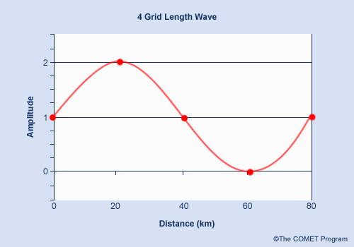
The previous example demonstrates that in some cases the information carried in full native grid NWP model data can be represented without much loss on output grids with lower horizontal resolutions. Ignoring the effect of numerical smoothers on model data for the moment, how far can we go toward representing model data on coarser and coarser output grids?
The example showed that there is little loss in going from a 22 km grid to a 40 km grid in the case of an atmospheric field - like the 1000 hPa vorticity – whose horizontal scale in terms of wavelength is on the order of 160-300 km.
Clearly the answer to the question of what output grid resolution can be used depends on the scale of the atmospheric phenomenon being considered: larger scales can be represented with more widely-spaced grid points.
Recall that waves will be aliased (incorrectly projected into longer wavelengths) if their wavelength is shorter than four grid lengths of the grid being used. This is true for a static representation of a wave on that grid. However, within an NWP model, a feature will be well-forecast in time only if its native grid is fine enough that at least eight grid lengths are used to define the feature.
For more discussion of this point, see the module “A 20 km Grid Depicts 40 km Features” in this series. In that misconception, the focus is on the horizontal resolution of the native grid of the forecast model. This discussion emphasizes the resolution of the output grids.
The four-grid length wave can provide us with a first rough estimate for how coarse a horizontal output grid can be while retaining model information without much loss. For a 1000 km wave (in the meso-alpha range), a 250 km grid spacing is the maximum. For a 100 km wave (in the meso-beta range) a 25 km grid spacing is the maximum. A 10 km wave (in the meso-gamma range) requires at least a 2.5 km grid.
This simple argument would suggest that atmospheric features with wavelengths in the 160-300 km range can be reasonably represented on a 40 km output grid, as noted in the example already presented. However, even in the absence of numerical smoothing, the four grid length rule suggests that such waves will be poorly-represented on the 80 km output grid. But remember that things are different when considering the native grid of the forecast model. For a numerical model with a native grid resolution of 40 km, features in the 160-300 km size range span fewer than 8 grid lengths, and so would likely be poorly predicted.
10. Full-Resolution Model Data are Always Required on Output Grids » Resolution versus Scale of Atmospheric Features (cont.)
Some features, such as small precipitation zones, could be considered as half waves in this simple treatment (they consist of a maximum with values dropping to zero on either side). Such small-scale precipitation features need high-resolution output grids to be accurately depicted.
For example, a band of precipitation 20 km wide (half of a full 40 km wave) would need at least a 10 km output grid according to our simple rule. But don’t forget that at such small scales, inadequacies in the model’s physics parameterizations and terrain representation can lead to incorrect forecasts on its native grid. No output grid can compensate for such difficulties.
For example, in convective situations, it is well known that due to inherent limitations in the convective parameterization scheme, a model can forecast convective precipitation areas with incorrect position and intensity.
On the other hand, higher-resolution NWP models have demonstrated skill in forecasting small-scale precipitation patterns related to orographic forcing. This point was discussed in the module “High Resolution Fixes Everything” in the 10 Common NWP Misconceptions series.
Precipitation forced by orography needs high-resolution output grids to be accurately depicted, and can be used with a certain degree of confidence in that case. Low-resolution output grids are of no use in depicting such precipitation.
10. Full-Resolution Model Data are Always Required on Output Grids » The Issue of Smoothers
The question of smoothing deserves a few words here. Numerical smoothers are applied for various reasons, and their effects depend on their type and strength. The forecaster should at least be aware of whether or not a smoother is applied to the data on the particular grid being used.
We have already seen that Eta model data are smoothed on the 211 80 km AWIPS grid, but not on the 40 and 20 km grids. In fact the smoothing on the 211 grid is characterized as “heavy”.
In Canada, GEM model data are available in GRIB format in two versions: high and low resolution. The high-resolution data are at the full horizontal resolution of the model. As of Dec, 2003, 24 km for the GEM regional model and 110 km for the GEM global model.
The low-resolution data are at approximately half the full horizontal model resolution: 60 km for the regional model and 220 km for the global model.
Other than the implicit smoothing caused by the interpolations, there is no smoothing used in the Canadian GRIB data.
Some effects of smoothing can be quite unexpected. For example, recall that it is possible to generate artificial supersaturation by averaging the mixing ratio and the temperature. This is because the exponential form of the Clausius-Clapeyron equation for saturation vapour pressure means that averaging two subsaturated states, one warm and one cold, can lead to supersaturation of the average.
This effect is illustrated at the 850 hPa level in the following two graphics. The first shows a large area of supersaturation due to this effect on the AWIPS 80 km 211 output grid, on which as we know the Eta model data are strongly smoothed.
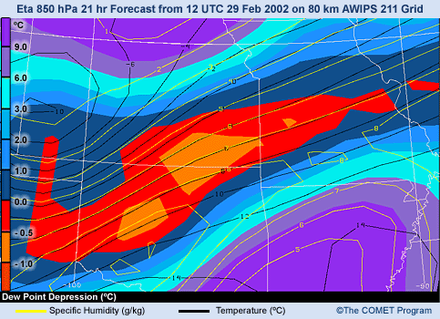
The second image shows the same variables on the 40 km 212 output grid. The artificial supersaturation effect is almost nonexistent on this grid, on which the model data are unsmoothed.
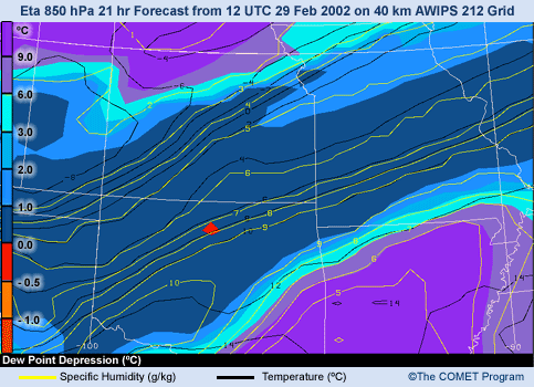
10. Full-Resolution Model Data are Always Required on Output Grids » Vertical Resolution
The question of the vertical resolution at which model data are available is also important. Various datasets can be available at various vertical resolutions, from the full model native grid resolution to something much coarser. The tendency over the years has been to increase NWP model vertical resolution, and correspondingly to increase the vertical resolution of the output grids.
This figure shows a tephigram with three superimposed profiles of temperature and dew point from Iqaluit, Nunavut, at 00UTC Oct 10, 2003. The black curves show the radiosonde observations and the green curves show the initial analysis of the GEM regional model at full vertical resolution (28 levels). The red curves show the same initial analysis, but on a reduced set of pressure levels in the vertical. A forecaster working with only the red profile of temperature would completely miss the warm air centred at around 800 hPa. This would have serious consequences for a forecast of precipitation type.
In practice this is not a concern for Canadian forecasters, since they receive GEM model output at full vertical resolution through BUFR format model profiles. However, those working on case studies with older or special datasets having limited vertical levels could potentially face this problem. For example, through December 2003, the GEM regional data available via Unidata did indeed include only a limited set of vertical levels.
10. Full-Resolution Model Data are Always Required on Output Grids » Vertical Resolution (cont.)
In cases in which there is a sloping tight gradient, such as a frontal zone, a vertical profile can be affected by horizontal smoothing and the interpolations used to transfer native model grid data to coarser horizontal output grids. As we already saw, such actions can lead to artificial supersaturation on the output grid. Certain profiles of temperature and dew point taken from the output grid will then show those supersaturated areas, where the dew point is greater than the temperature.
One final point about vertical resolution is worth mentioning. It relates to the terrain representation effect in complex terrain.
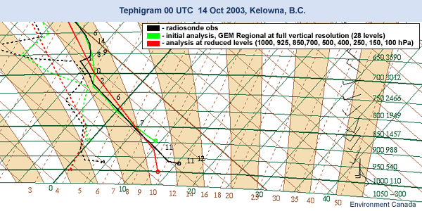
This figure shows a tephigram from Kelowna, BC, from 00UTC Oct 14, 2003. In it we see that the radiosonde observation places Kelowna at about 965 hPa, with a temperature of 15ºC and a dew point close to 5ºC. The model sounding at low resolution on standard pressure surfaces extrapolates the two curves downward to the 1000 hPa level.
Note that the full-resolution model profiles place Kelowna at about 900 hPa, with a temperature of 9ºC and a dew point just under 0ºC. This is an illustration of the terrain representation effect: even with full-resolution model vertical profiles, the user in complex terrain cannot rely on the model for accurate values of variables near the surface.
Of course, as model horizontal resolution increases, the terrain representation issue becomes less of a problem, since the model terrain becomes correspondingly better defined. Further discussion of the terrain representation effect can be found in “NWP Models Directly Forecast Near-Surface Variables” in this series.
In general, forecasters should consider NWP model data with full resolution in the vertical. This is because vertical variations in atmospheric variables can occur over very short distances. Datasets with low vertical resolution may lead the forecaster down the path of error.
10. Full-Resolution Model Data are Always Required on Output Grids » Test Your Knowledge
Question 1
Question
Is a feature with a wavelength of 200 km able to be well-forecast by the GEM regional model (native grid horizontal resolution 24 km)?
The correct answer is Yes
To be well-forecast, a wave must be represented by at least 8 gridpoints in the horizontal on the native grid of a numerical model. Therefore, we can estimate that waves of 8X24 km or larger will be well-forecast.
Note: The answer to this question is based on application of a simple rule and should be considered no more than a rough estimate. In reality, no sharp cutoff can be defined.
Question 2
Question
Is a feature with wavelength of 200 km well-depicted on the output grid of the GEM regional low-resolution GRIB data (60 km resolution)?
The correct answer is No
These GRIB data are at a horizontal resolution of 60 km. Using the four-grid length rule for output grids, we know that features with wavelengths greater than 240 km can be depicted on a 60 km grid.
Note: The answer to this question is based on application of a simple rule, and should be considered no more than a rough estimate. In reality, no sharp cutoff can be defined.
10. Full-Resolution Model Data are Always Required on Output Grids » Reality
Because of considerations of speed and economy, full-resolution model datasets are not always made available to the forecast community. We have seen that in some cases this is an acceptable practice, while in others it can cause problems.
In general, the accuracy of representation of a feature on a given output grid depends upon the horizontal scale of the feature. Relatively large features, with scales on the order of 1000 km, will be correctly depicted at any of the horizontal resolutions used in common output grids. Smaller features require finer output grids to be correctly depicted.
We have seen that a wavelike feature will be well-depicted on a horizontal output grid if its wavelength is longer than four grid lengths of that grid. However, when considering the NWP model itself, features other than those tied to orography, such as orographically-forced precipitation, must have a wavelength at least eight times larger than the resolution of the native model grid. Otherwise, the model forecast itself is likely to be inaccurate.
A complicating factor is that smoothing may be done as part of the process of transferring NWP data from model grids to output grids. In addition to knowing the resolution of the output grid, the forecaster should be aware of what smoothing if any has been applied to the data on that grid.
Vertical resolution of output grids is also important. Using low-resolution vertical grids exposes the forecaster to the risk of misinterpretation of what the model is doing. Low-resolution grids can easily miss important features in the vertical. Forecasters should always try to work with full-resolution model vertical profiles. Those using older or special output grids with lower-than-native vertical resolution will have to proceed with care.
The forecaster in complex terrain is faced with an additional challenge: due to the terrain representation effect, the model cannot supply accurate vertical profiles near the ground, even at full model vertical resolution.
To learn more about this topic, visit Influence of Model Physics on NWP Forecasts, a module of the COMET NWP Distance Learning Course.
Contributors
COMET Sponsors
Sponsors
- Meteorological Service of Canada (MSC)
- National Weather Service (NWS)
- National Oceanic and Atmospheric Administration (NOAA)
To learn more about us, please visit the COMET website.
Project Contributors
Principal Science Advisor
- Stephen Jascourt — UCAR/COMET
- Bill Bua — UCAR/COMET
Project Lead/Instructional Design
- Bruce Muller — UCAR/COMET
- Patrick Parrish — UCAR/COMET
Project Meteorologist
- Garry Toth — MSC
Multimedia Authoring
- Bruce Muller — UCAR/COMET
- Dan Riter — UCAR/COMET
- Carl Whitehurst — UCAR/COMET
Audio Editing/Production
- Seth Lamos — UCAR/COMET
Audio Narration
- Garry Toth — MSC
- Dominique de LaBruère Toth
Computer Graphics/Interface Design
- Heidi Godsil — UCAR/COMET
Illustration/Animation
- Steve Deyo — UCAR/COMET
Software Testing/Quality Assurance
- Michael Smith — UCAR/COMET
Copyright Administration
- Lorrie Fyffe — UCAR/COMET
Data Provided by
- MSC
- NWS — NOAA
COMET HTML Integration Team 2021
- Tim Alberta — Project Manager
- Dolores Kiessling — Project Lead
- Steve Deyo — Graphic Artist
- Ariana Kiessling — Web Developer
- Gary Pacheco — Lead Web Developer
- David Russi — Translations
- Tyler Winstead — Web Developer
COMET Staff, Summer 2002
Director
- Dr. Timothy Spangler
Assistant Director
- Dr. Joe Lamos
Meteorologist Resources Group Head
- Dr. Greg Byrd
Business Manager/Supervisor of Administration
- Elizabeth Lessard
Administration
- Lorrie Fyffe
- Bonnie Slagel
Graphics/Media Production
- Steve Deyo
- Heidi Godsil
- Seth Lamos
Hardware/Software Support and Programming
- Steve Drake (Supervisor)
- Tim Alberta
- Carl Whitehurst
Instructional Design
- Patrick Parrish (Supervisor)
- Dr. Alan Bol
- Lon Goldstein
- Dr. Vickie Johnson
- Bruce Muller
- Dr. Sherwood Wang
Meteorologists
- Dr. William Bua
- Patrick Dills
- Doug Drogurub (Student)
- Kevin Fuell
- Jonathan Heyl (Student)
- Dr. Stephen Jascourt
- Matthew Kelsch
- Dolores Kiessling
- Dr. Richard Koehler
- Wendy Schreiber-Abshire
- Dr. Doug Wesley
Software Testing/Quality Assurance
- Michael Smith (Coordinator)
National Weather Service COMET Branch
- Richard Cianflone
- Anthony Mostek (National Satellite Training Coordinator)
- Elizabeth Mulvihill Page
- Dr. Robert Rozumalski (SOO/SAC Coordinator)
Meteorological Service of Canada Visiting Meteorologist
- Peter Lewis
- Garry Toth