Produced by The COMET® Program
Introduction
This is part two of the two-module series on estimation of observed precipitation.
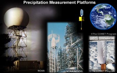
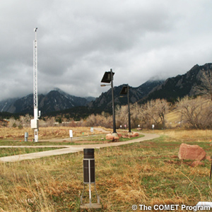
The first module focused on measurement: understanding measurement sensors—radar, satellite, and rain gauges—along with precipitation climatology tools.
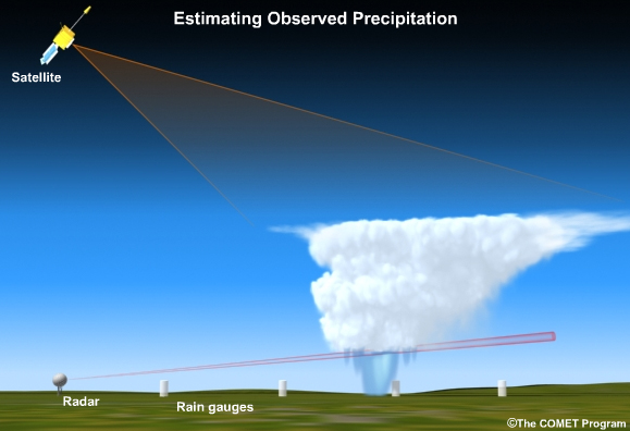
In this module, we’ll focus on how to make the best use of different precipitation measurements for an analysis. The ultimate goal is to develop a blended product that combines the best of radar, satellite, and rain gauge measurements for an optimal analysis of observed precipitation. The module draws on the experience of forecasters in NOAA’s National Weather Service (NWS) to suggest the best way to do this.
Related training is also available through the NOAA Warning Decision Training Branch (WDTB).
Multisensor Precipitation Estimator Product Training, NOAA/WDTB
http://www.wdtb.noaa.gov/buildTraining/FFMP-A/MPE/player.html
Multi-sensor Precipitation Estimator (MPE)
In the United States, NOAA’s NWS uses a program called the Multisensor Precipitation Estimator, or MPE. MPE allows forecasters the flexibility to address the variety of issues encountered when trying to develop accurate and timely estimates of observed precipitation.
MPE consists of two core programs: MPE Field Generation and MPE Editor. The Field Generation generates data for display. The editor is the primary user interface that allows the forecaster to evaluate and edit the precipitation analyses. Using the edited data, the Field Generation can be re-run to generate new MPE products. In this module, we will focus on effective use of the MPE Editor.

MPE’s primary purpose is to combine the most desirable aspects of each precipitation estimation platform; radar, satellite, and gauges, into one precipitation analysis. These estimates may be enhanced with climatology where appropriate.
- Radar and rain gauge often most influential on MPE product
- However, radar less reliable for
- Regions of rugged terrain
- Events dominated by snow
Of the three precipitation measurement platforms, the radar and rain gauge data are usually the most influential on the final MPE product. However, there may be less reliance on radar in regions of rugged terrain and in events dominated by snow.
MPE products show liquid precipitation plus the liquid equivalent of frozen precipitation.
Other Precipitation Estimation Programs
Programs incorporated into MPE:
- Mountain Mapper’s Daily QC
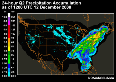
- National Mosaic and Multi-sensor QPE (NMQ)
- Referred to as “Q2"
Within the hydrometeorological community in the United States, several other programs have been used over the years that address QPE. Although these were developed independently of MPE, the functionality of two key programs has been incorporated into MPE. These are Mountain Mapper’s Daily QC program, and the National Mosaic and Multi-sensor QPE (NMQ), most commonly referred to as Q2.
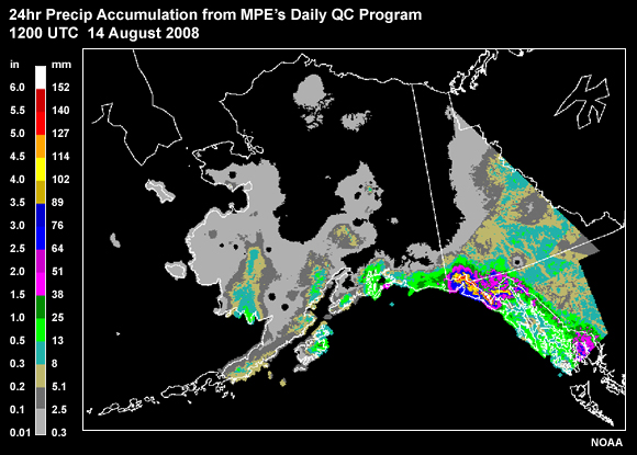
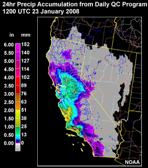
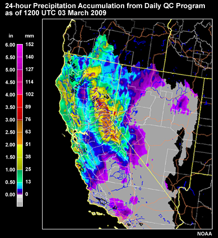
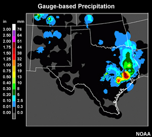
Daily QC: QPE with quality-controlled, or “QC’d” gauge observations and precipitation climatology.
Mountain Mapper has been in use by River Forecast Centers (RFCs) in the West where orographic forcing can play a big role in precipitation distribution. The Daily QC part of that system generates QPE using available quality-controlled, or “QC’d” gauge observations and precipitation climatology. This Daily QC function is part of the MPE suite of functions.
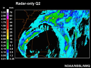
NOAA's National Severe Storm Laboratory radar-derived precipitation product (part of NMQ Q2 program) is a dataset available to MPE
Thus, Q2 functionality, especially the hourly radar-based accumulation, is a dataset available to MPE.
MPE Methodolgy
The MPE methodology may vary from region to region, and even from season to season within a region. But the basic methodology when good radar coverage exists will include the following:
1. Locate and differentiate areas of general rain, convective rain, hail, snow, virga and melting precipitation.
2. Evaluate gauge data and correct bad reports.
3. Re-generate and re-evaluate the different radar-based QPE fields after the gauge quality control is performed.
4. Correct remaining problem areas with editing tools, including polygon edits.
5. Correct inaccuracy that may become apparent later when more data are available.
Step 1: Differentiate areas of general rain, convective rain, hail, virga, snow, bright band, and radar blockage areas.
Step 2: Evaluate gauge data and make necessary edits
Step 3: Re-evaluate precipitation fields after gauge edits
Step 4: Correct remaining problems, possibly with polygon edits
Step 5: Adjust precipitation analyses with data that comes in later
This five step process is especially useful when good radar coverage exists.
For regions and seasons with areas of poor radar coverage, there may be a few differences in the process.
For frozen precipitation, it’s likely that none of the radar-based products provide suitable QPE. After steps 1-2, the most efficient option may be to gather as many liquid equivalent reports as possible and produce a gauge-based QPE. This QPE may get updated with additional data as described in step 5.
For regions with large areas of radar blockage, the best estimates may be from climatology-adjusted, gauge-based QPE.
This PRISM-adjusted QPE product is an example. If a region has a dense gauge network and some areas of good radar coverage, QPE can take advantage of both in a multiple sensor mosaic.
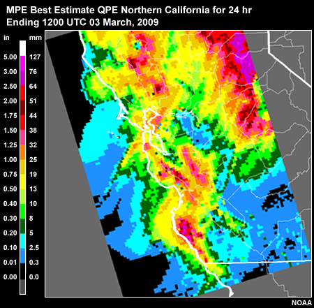
This MPE product takes advantage of radar where it can, and uses PRISM-adjusted gauge information elsewhere.
In This Module
More recent developments and manuals as of 2020 can be found on the Office of Hydrologic Development website:
https://www.nws.noaa.gov/oh/hrl/general/indexdoc.htm
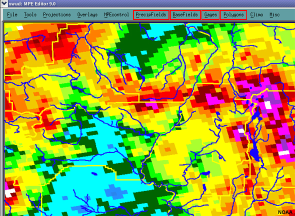
This module will not be a tutorial on running MPE, but rather will provide an overview of the scientific issues impacting effective use of the application.
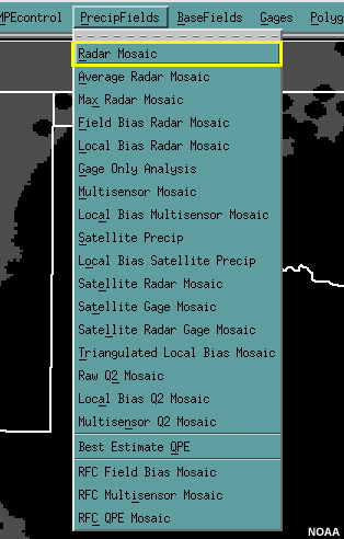
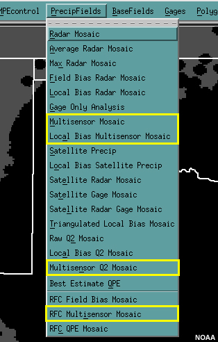
As we work through sections 2-5, we will focus on some of the products available under the PrecipFields, BaseFields, Gages, and Polygons menus.
More recent developments and manuals as of 2020 can be found on the Office of Hydrologic Development website:
https://www.nws.noaa.gov/oh/hrl/general/indexdoc.htm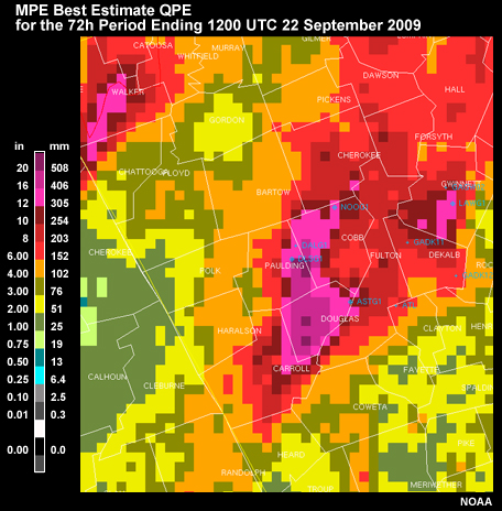
- Section 2: Information in Precipitation Fields, including:
- Bias-adjusted fields
- Multisensor fields
- Section 3: Tools for evaluating and editing data:
- Section 4: MPE Case Study Examples
- Section 5: Summary
Section 2 discusses some of the important information in the MPE Precipitation Fields. This includes the bias-adjusted and multisensor fields.
Section 3 reviews some important tools for evaluating and editing the precipitation information.
Section 4 provides MPE case study examples.
Section 5 provides a module summary.
Precipitation Fields
Automated MPE products provide precipitation analyses:
- From each source: radar, gauges, and satellite
- Adjusted for bias in the radar or satellite fields
- Based on blended multisensor information
The MPE editor PrecipFields menu provides access to a number of accumulation products. These products are based on automated procedures and together they provide:
-
Precipitation analyses from each source—radar, gauges, and satellite
-
Precipitation analyses adjusted for bias in the radar or satellite fields
- Precipitation analyses based on blended information from multiple sensors.
In this section we will explore a few select products in order to explain scientific issues common to all of the products.
MPE Precipitation Field Options
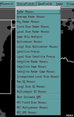
Although there are only three measurement platforms—radar, gauges, and satellite you can see there are many more than three precipitation fields to choose from. And the list is likely to grow in future versions of MPE.
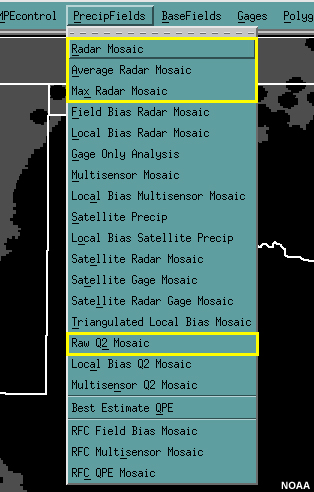
We will group these fields to focus on some of the underlying scientific issues. Group one will be those products based on radar-only QPE. These include NMQ’s Q2.
Group 2 will look at the gauge-only QPE.
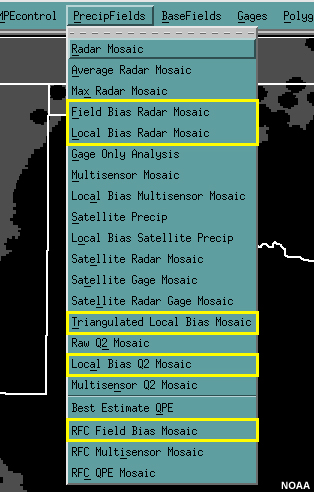
Group 3 will go over the concept of gauge-generated bias adjustments for radar QPE.

Group 4 will look at multisensor analyses that use radar and gauge QPE.
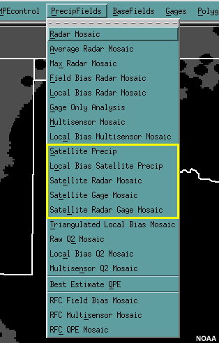
Group 5 contains products that use satellite QPE.
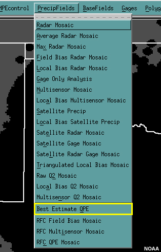
Best Estimate QPE:
- Set by forecaster to save the best possible gridded precipitation estimate that hour
- Consists of one of existing products with user edits and alterations
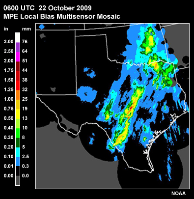
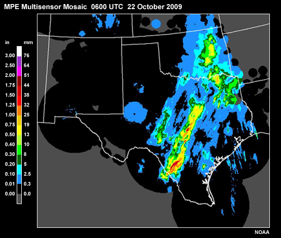
- By default set to Multisensor Mosaic (Build 9.2)
The Best Estimate QPE is simply what the forecaster believes to be the best possible gridded precipitation estimate that hour. It is therefore one of the existing products, with whatever edits and alterations the forecaster may have made before saving. As of MPE Build 9.2 it is set by default to the Multisensor Mosaic. An RFC can change the default Best Estimate QPE to any of the other Precip Fields based on event, season, location, etc. See the User’s Guide for more information.
Radar QPE Input: MPE Radar Mosaics
Radar data provide useful QPE info:
- Timing
- Spatial distribution
- Best for convective, liquid precipitation
Radar data supply very useful information about timing and spatial distribution of precipitation. Radar QPE is particularly useful for liquid precipitation, especially convective systems.
As a starting place for radar QPE, there are several options within MPE. Although the radar data come from the same radars, there are different ways the data are processed to arrive at the raw precipitation estimates. One of those is the radar QPE field called Radar Mosaic.
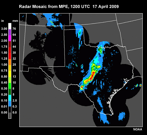
It is obtained directly from the NWS’s Digital Precipitation Array (DPA) and displayed on the Hydrologic Rainfall Analysis Project (HRAP) grid. There is no gauge-generated bias correction.
RMosaic data meets criteria:
- Considered good coverage by radar climatology
- Lowest elevation radar is used
Data displayed in Radar Mosaic meet two criteria:
One, the data are considered usable if the Radar Climatology guidance (described in Precipitation Estimates Part I, section 2) indicates good coverage.
Two, if an HRAP grid bin is covered by more than one radar, the radar which provides the lowest elevation coverage is used. The philosophy is that the lowest possible radar sample will most closely match the precipitation reaching the ground.
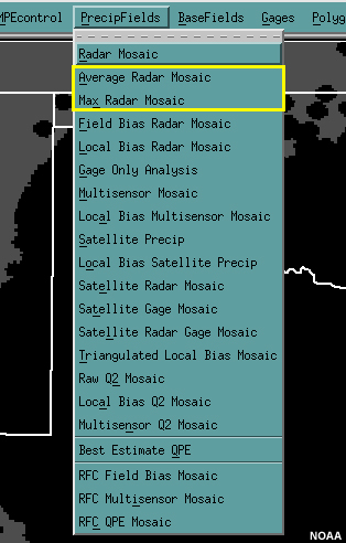
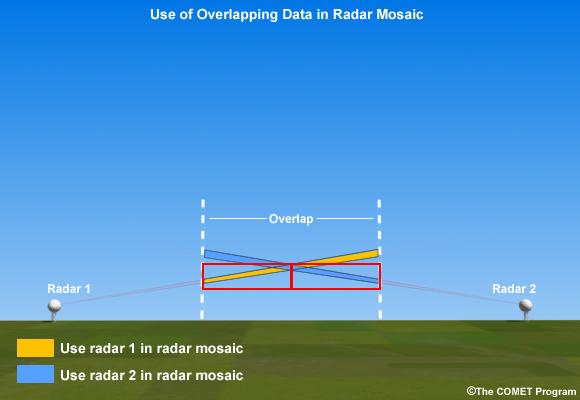
There are other radar QPE mosaics that can be used as a starting point in MPE. These include the Average Radar Mosaic and Max Radar Mosaic. Like Radar Mosaic, these contain raw precipitation estimates and are generated in areas that have reliable coverage according to the Radar Climatology guidance. The difference is in how areas of radar overlap are handled.
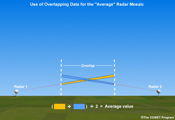
Average Radar Mosaic uses the average of different radar values in areas of overlap. This product is sometimes used to help smooth out abrupt differences between radars.
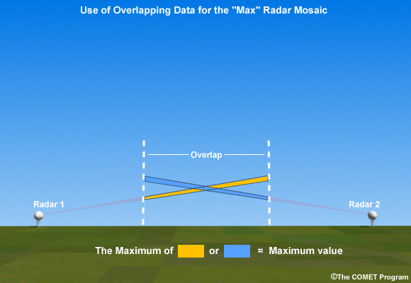
Max Radar Mosaic uses the maximum value of the different radar values in areas of overlap.
Radar QPE Input: NMQ Q2
NOAA/NSSL NMQ site: http://www.nssl.noaa.gov/projects/q2/
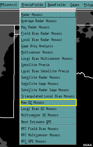
An alternate source of radar-derived QPE for MPE input is NMQ’s Q2.
Some of the processing techniques used in the Raw Q2 Mosaic are different than those used in the Radar Mosaic. More detail can be found at the website.
- Dynamic Z-R relationships based on reflectivity characteristics
- Better clutter suppression.
- Range coverage out to 460 km
Among the highlights of the Raw Q2 Mosaic that may be useful when compared to Radar Mosaic:
- Dynamic Z-R relationships that are based on the vertical profile of radar reflectivity.
- Clutter suppression techniques that work better in some areas.
- Range coverage out to 460 km.
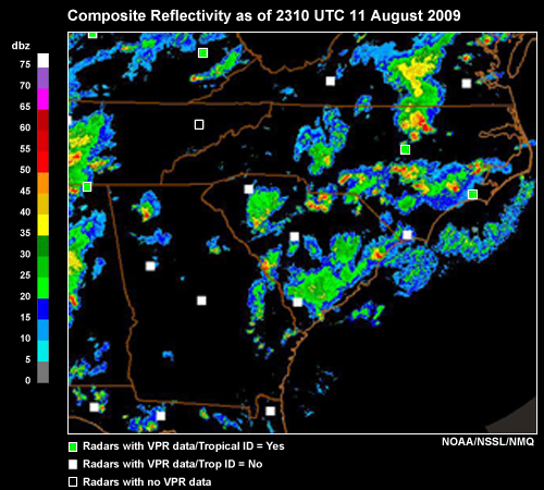
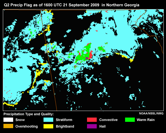
The dynamic Z-R equation function of Q2 uses the vertical profile of reflectivity, to infer characteristics of precipitation production. The green squares indicate radars with areas that exhibit some tropical or warm rain characteristics. The warm rain Z-R coefficients are used in these areas.
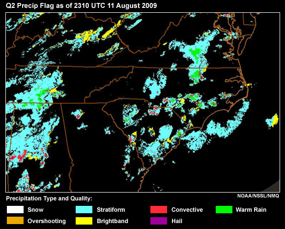
The corresponding Q2 Precip Flag shows different areas of similar precipitation characteristics. Each area uses Z-R coefficients appropriate for the precipitation there. The green shaded areas are where the warm rain Z-R is used.
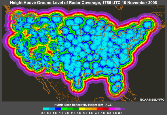
Although some users like the greater range coverage, keep in mind that just because the data extend beyond 230 km, the data are not necessarily useful. The yellows through reds on this map depict areas where radar sampling is more than 3 km above the ground. Only well-developed, deep, convective clouds are likely to be sampled at such elevations. Even in the dark blue and green areas where the radar sample is more than 1 km above the ground, there may be problems with precipitation sampling in stratiform and low-centroid convective clouds.
NOAA/NSSL NMQ site: http://www.nssl.noaa.gov/projects/q2/
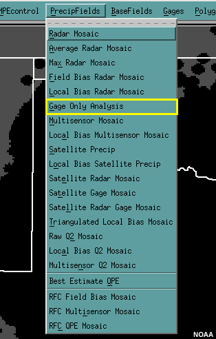
Gauge-Only Field
This Gage Only Analysis results in a field that’s based on only the gauge reports, along with a precipitation climatology adjustment.

There are settings within MPE that determine the radius of influence of a gauge report, as well as whether a report of 0.00 will be considered even if the radar at that location suggests a non-zero amount. The current MPE defaults are for a radius of influence around the gauge of 15 HRAP bins, or about 60 km.
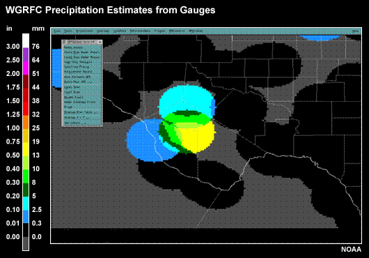
In areas of sparse gauge density, the gauge value is spread throughout the entire radius of influence. “Missing” values are assigned to bins outside the radius of influence of any gauge.
When the gauge density increases enough so that there are overlapping radii of influence, distance weighting is applied to the gauge value. For example, a bin halfway between two gauges and within the radius of influence of each gauge will have a value that is the average between the two gauge reports. If the bin is closer to gauge 1, but still under the radius of influence from gauge 2, the value will be a blend of the two, but with greater influence from gauge 1.
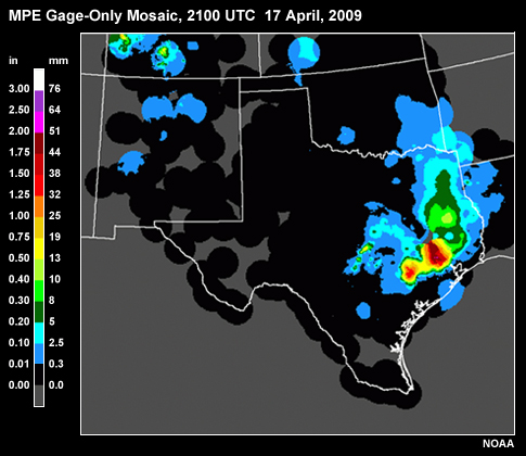
With dense gauge networks, we start getting gauge-only fields that look like this one.
The Gage Only Analysis is adjusted by precipitation climatology, such as the PRISM data. This will be more apparent in the West where orographic influences have a greater impact on precipitation distribution.
Gauge-Adjusted Radar Exercise
- Methodology 1: use gauges to compute a bias correction for the radar QPE
- Field bias: one bias correction for entire radar coverage
- Local bias: bias correction for each grid bin
- Methodology 2: merge radar QPE and gauge reports into a multisensor mosaic
There are a number of MPE precipitation fields that adjust radar QPE using quality-controlled gauge reports. But there are only two primary methodologies for doing this adjustment.
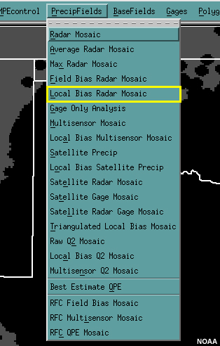
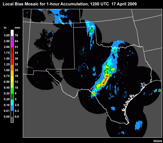
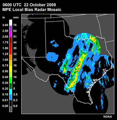
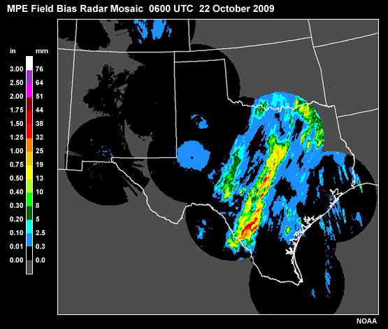
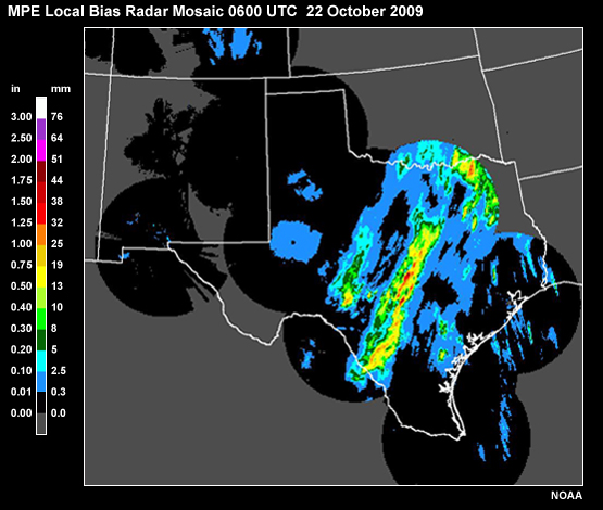
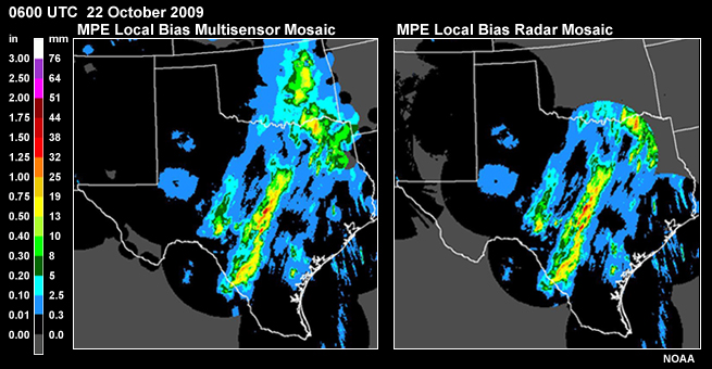
1) Use gauge reports to compute a correction factor, or bias, for the radar QPE as we see in the Local Bias Radar Mosaic:
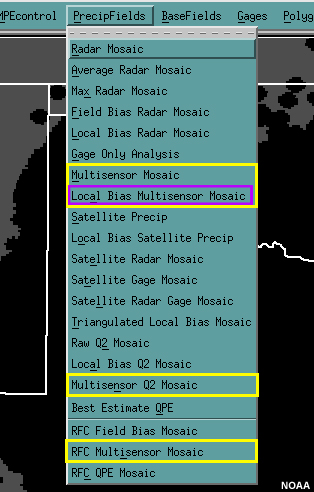
Or, 2) merge the radar QPE with rain gauge reports to get a multiple sensor QPE as we see in the Local Bias Multisensor Mosaic:
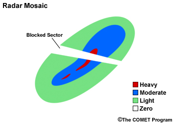
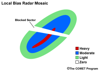
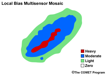
Now, let’s take a look at three idealized scenarios: a Radar Mosaic, a bias-corrected field such as the Local Bias Radar Mosaic, and a multiple sensor field such as the Local Bias Multisensor Mosaic.
Assume we have an adequate distribution of accurate gauge reports for the hour.
Compare each idealized scenario with the true QPE. Note how they compare with the “truth” and with each other.
Question 1 of 2
Which one seems to have the closest magnitudes to the “truth” and preserves
the radar QPE coverage?
Choose the best answer.
The correct answer is a) Local Bias Radar Mosaic
Question 2 of 2
Which one seems to have the closest magnitude to the "truth" when
considering both the good and bad radar coverage areas?
Choose the best answer.
The correct answer is b) Local Bias Multisensor Mosaic
Mean Field Bias
Field bias computation:
- Requires minimum number of non-zero gauge-radar comparisons
- Gauge radar pairs from anywhere in good coverage area
- Use pairs from previous hours to reach the minimum number
Bias Value = Avg. of Gauges ÷ Avg. of Radar for all gauge-radar pairs
So let’s review a little more detail regarding the science in the bias-corrected radar QPE. Computing the bias correction factor requires a minimum number of comparisons between the gauge reports and the radar QPE at the gauge locations. These gauge-radar comparisons, called gauge-radar pairs, are for locations where both the gauge and the radar indicate non-zero values. This is set to 10 pairs by default. Fewer pairs can increases the risk of inaccurate bias corrections.
For the Field Bias Radar Mosaic, those pairs can come from anywhere in the radar coverage area.
And if the minimum number of pairs is not obtained in a particular hour, the program will use pairs from previous hours to reach that number. Weighting factors are applied so that older data have less influence. The actual bias value is the average of the gauge values divided by the average of the radar values for all of the gauge-radar pairs.
Question 1 of 2
A gauge-radar pair is _____.
Choose all that apply.
The correct answers are b) and c)
Question 2 of 2
Under what conditions would the single field bias correction be useful?
Choose the best answer.
The correct answer is c) Area-wide radar calibration problem
Field bias correction works best when a uniform bias exists across the entire area of good radar coverage.
Field bias correction best for uniform problems, such as radar calibration issue
Field bias correction works best when a uniform bias exists across the entire area of good radar coverage.
Local Bias
Local bias computation:
- Gauge radar pairs from within local radius of influence
- Minimum number of non-zero gauge-radar comparisons
- Use pairs from previous hours to reach the minimum number
- Advantage: can account for local conditions and storm characteristics
- Disadvantage: bias correction may be computed with data that is spread over multiple hours
The Local Bias Radar Mosaic computes a bias correction the same way but the gauge-radar pairs come from within the radius of influence of a gauge. Once again, there is a minimum number of pairs required, often set to 10, and the program will look back at previous hours to reach the minimum number of pairs.
An advantage of this type of bias correction is that theoretically it can account for changing conditions and storm characteristics by using the local comparisons between the gauge reports and the radar QPE.
A disadvantage is that it is more difficult to get the minimum number of gauge radar pairs in a local area. As a result, the 10 pairs may spread over a long period of time, perhaps many hours. In that time period the local conditions could change significantly rendering the local bias correction factor irrelevant.
Question
Under what conditions would the local bias corrections be most useful?
Choose the best answer.
The correct answer is b) Convective rain in one part of the area and stratiform rain in another
The local bias adjustment is intended to adjust the radar QPE based on local conditions and storm characteristics. Blockage cannot be corrected with bias adjustments. Snow and sleet are often inadequately represented by radar-based fields.
- Adjust radar QPE based on local conditions
- Radar blockage is not corrected
- Snow QPE is often inadequate
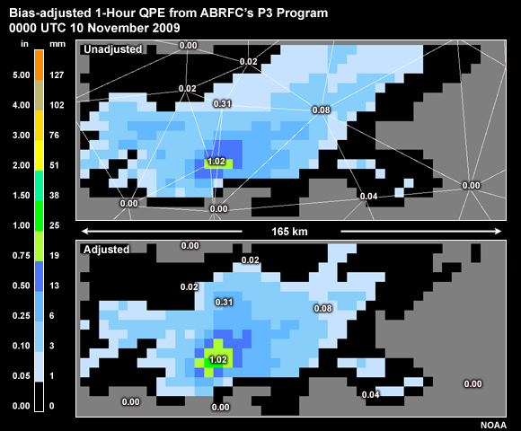
The Arkansas Basin River Forecast Center sometimes uses a method that creates a Triangular Irregular Network, or TIN, with the gauges. The TIN is used to distant weight the gauge and corresponding radar values when creating a local bias correction factor. The method requires a dense gauge network. After the correction, the grid values better match the reports of 1.02 and 0.31 in (26 and 8 mm).
Multisensor Fields
The merging of QPE from multiple sensors is typically seen as the final step in the science behind radar-based QPE. Although multisensor mosaics can use satellite as one of the sensors, currently the most common approach is to use a radar and rain gauge combination. That’s what we will focus on here, but you are encouraged to consult the NWS MPE Users Guide for more information about those products that use satellite.
The merging of gauge and radar data into one product is the basis for these PrecipFields selections. Differences in the menu options have to do with which radar QPE field you start with.
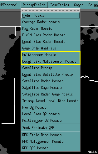
- Focus on multisensor fields that merge gauge and radar QPE
- Multisensor Mosaic = Field Bias Radar Mosaic + Gage Only Analysis
- Local Bias Multisensor Mosaic = Local Field Radar Mosaic + Gage Only Analysis
We will focus on these two multisensor mosaics because the others follow the same scientific philosophy. The Multisensor Mosaic is the merging of the Field Bias Radar Mosaic and the Gage Only Analysis. The Local Bias Multisensor Mosaic is the merging of the Local Bias Radar Mosaic and the Gage Only Analysis.
The gauge values in a multisensor mosaic are used as anchoring points at the gauge locations.
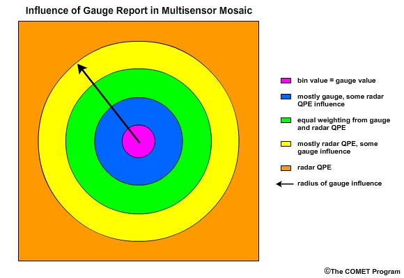
Multisensor Mosaic can alter relative values and spatial distribution of the radar QPE.
The grid bin associated with the gauge location must be the gauge value. For grid bins not directly associated with a gauge report, the value is based on blending the radar QPE value and the distance-weighted value from the gauge analysis. As you get further from the gauge location, the radar QPE value will become more dominant until you are beyond the influence of the gauge and use only the radar QPE. With the merging of the gauge data, the Multisensor Mosaic can alter the relative values and spatial distribution of the radar QPE.
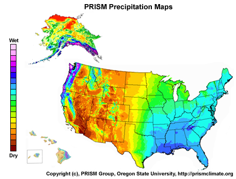
Climatology can impact gauge QPE and thus the Multisensor Mosaic too. Currently, the PRISM-adjusted gauge analyses have a strong impact on multisensor analyses in regions with sharp terrain features and poor radar coverage.
Bias Correction versus Multisensor
Comparison of Multisensor Products vs. Bias-adjusted Products:
| Multisensor Products | Bias-adjusted Products |
|---|---|
| Can fill in areas with missing radar QPE | Only values where radar QPE exists |
| Grid box value at gauge location equals gauge value | Grid box value at gauge location does not always equal gauge value |
| Spatial detail and relative values of radar QPE may be altered | Spatial detail and relative values of radar QPE preserved |
| Performed with very few gauges | Minimum number of gauge-radar pairs required |
To summarize, there may be some important benefits to the different bias-adjusted radar QPE mosaics. But the bias-adjusted fields are often viewed as an intermediate step on the way to one of the multisensor products as the final QPE. Here is the Local Bias Multisensor Mosaic which is based on the Local Bias Radar Mosaic.
The table compares the bias-adjusted product characteristics with the multisensor product characteristics. A bias-adjusting approach may be the approach of choice if it is important to preserve the exact spatial detail of the radar QPE.
Otherwise, the multisensor techniques have the advantage of using gauge data to fill in areas of poor, or missing, radar coverage while using information from bias-adjusted radar QPE in other areas.
The multisensor approach also forces the QPE grid to match the gauge report at gauge locations and can be performed with fewer gauges.
Keep in mind, a single bad gauge report can have a large impact on a multisensor mosaic, so careful gauge QC is essential.
Satellite QPE
Satellite QPE fields can be used either as is or with a gauge-based bias correction. Satellite QPE can also be part of a multisensor field. When radar and satellite QPE are used in the same multiple sensor field, the satellite QPE is only used where radar QPE is unavailable due to poor radar coverage.
As of 2009 the satellite products are not frequently used due to issues with accuracy and spatial resolution.
Review Questions
Question 1 of 6
The difference between Radar Mosaic, Max Radar Mosaic and
Average Radar Mosaic is in
_____.
Choose the best answer.
The correct answer is c) how areas of overlap are handled
Question 2 of 6
The radar QPE field known as Q2 differs from the Radar Mosaic in that
_____.
Choose all that apply.
The correct answers are a) and c)
Question 3 of 6
The Gage-Only Analysis does not consider precipitation climatology.
Choose the best answer.
The correct answer is b) False
Question 4 of 6
The local bias adjustment is computed from gauge reports that _____.
Choose all that apply.
The correct answers are b) and d)
Question 5 of 6
Unlike the bias-corrected mosaics, the multisensor mosaics _____.
Choose all that apply.
The correct answers are a) and d)
Question 6 of 6
A vital assumption for the input to all of the bias-corrected and multisensor QPE
fields is the _____.
Choose the best answer.
The correct answer is d) gauge reports are accurate and representative
Quality Assessment and Adjustments of Data
In this section:
- Options for data
- Evaluation
- Editing
This section focuses on some of the options for data evaluation and editing found in the Gages, Basefields, and Polygons menus of the MPE editor. Those in the Gages menu are used for displaying, evaluating, and possibly altering gauge data. In the Basefields menu we will focus on the options for determining the representativeness of the gauge-generated bias adjustments. The Polygons menu is where the user can use the polygon tool to edit MPE data.
Gauge data QC vitally important because they are used for:
- Computing bias corrections to radar and satellite
- Anchoring points of “ground truth” for QPE in multisensor products
- Ground observation for climo-adjusted QPE in radar-blocked areas
The quality of rain gauge data is vitally important for precipitation analyses such as those performed within MPE. Gauge data are used to compute bias corrections to radar and satellite QPE. They are the anchoring points of “ground truth” for QPE in the multisensor products. They are also the anchoring points of ground observation for climatology-adjusted QPE often used in radar-blocked areas through either the gauge only or multisensor products.
Gauge Data Evaluation & Quality Control
- MPE treats QC’d gauge data as ground truth
- Bad data adversely affects MPE PrecipField
Although there are error sources in all forms of precipitation measurement, MPE treats quality-controlled gauge data as ground truth.
If poor quality gauge data make it through the quality control checks, these data can adversely affect many of the precipitation fields that depend on accurate and spatially representative reports of rain and liquid equivalent of frozen precipitation.
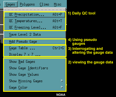
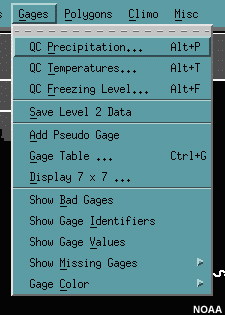
MPE offers a suite of tools for assessing, adjusting, and if necessary, removing gauge data. The MPE User’s Guide can assist with details of selections within the Gages menu. For this training, the Gages menu options are divided into four groups: (1) the Daily QC tool, (2) viewing the gauge data, (3) interrogating and altering the gauge data, and (4) using pseudo gauges.
Daily QC and QC Precipitation
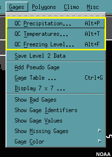
MPE’s QC Precipitation, QC Temperatures, and QC Freezing Level are based on the Daily QC function.
Daily QC is a component of the Mountain Mapper Program. It is used primarily in the West to produce precipitation analyses for input to river models.
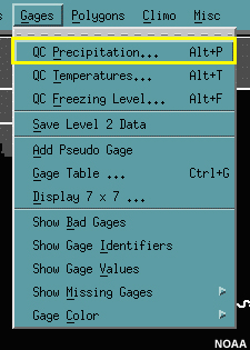
We will focus on the QC Precipitation menu option.
Gauge-based QPE, adjusted with precipitation climatology, is useful in regions where mountainous terrain greatly affects the distribution of precipitation while at the same time reducing the effective radar coverage.
The QC Precipitation option uses the available gauge data and performs spatial and temporal checks. Gauges are flagged “questionable” but not removed if they don’t pass these checks. The forecaster may choose to further evaluate these questionable values.
As of MPE Build 9.2, QC Precipitation is for 6 and 24 hour time durations. However, during the “save” step in MPE, the data can be disaggregated into 1-hour time steps for some stations.
Viewing Gauge Data
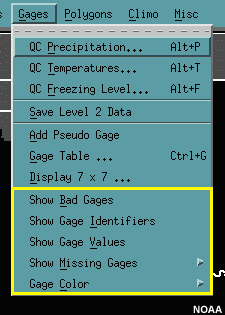
This group in the Gages menu provides map display options that allow the forecaster to make a quick assessment of the gauge field. One approach can be as simple as looking at the plotted gauge values to pick out any outliers.
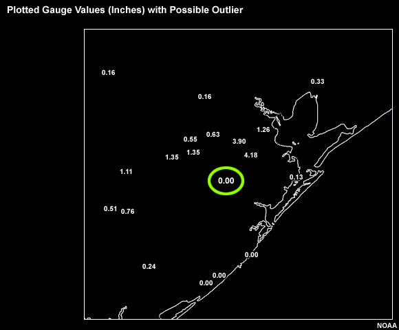
This zero value in a region of significant non-zero values may seem to be in error.
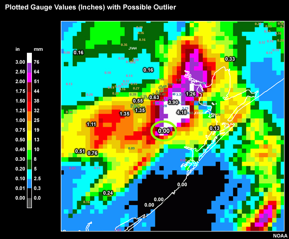
Overlaying a radar-derived precipitation plot further confirms that this should probably not be a zero value.
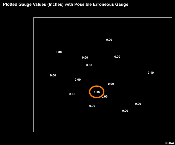
This large value of 1-hour precipitation surrounded by minimal values also appears to be in error.
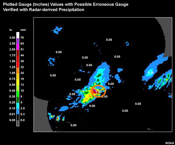
Here the radar-derived precipitation may be used to confirm that the outlier gauge report may be valid.
Functions within the MPE gauge data processing can help with automatically identifying outlier, or suspicious gauge reports. Remember that the first of two core programs within MPE, MPE Field Gen, performs automated quality control checks on all of the hourly gauge reports.
Gauges that fail to pass the QC checks are flagged but not automatically removed. They can be manually removed by forecasters using the MPE Editor or remain available for further computations.
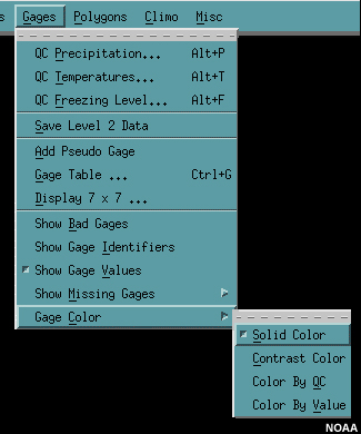
The colors of the plotted gauge values can be based on how they did in the automated QC checks. This option, Color by QC, is reached from the gages menu.
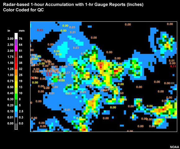
For example, gauges are flagged in yellow or red to indicate inconsistencies with radar or neighboring gauges.
Red ones are non-zero gauge reports. Yellow ones are zero gauge reports. The user has the option to remove any of these gauges from further computations.
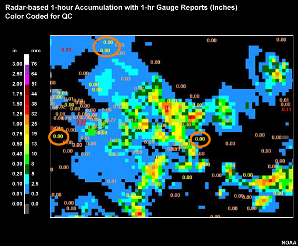
You can see here that some of the zero reports don’t seem to be outliers. They may be in areas where the radar is sampling virga (as shown in top circle).
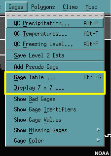
Interrogating Gauge Data: “Gage Table”
This group in the Gages menu permits more gauge-specific detail when assessing gauge values.
Gauge table allows forecaster to:
- Interrogate gauge value
- Compare gauge value to MPE grid value
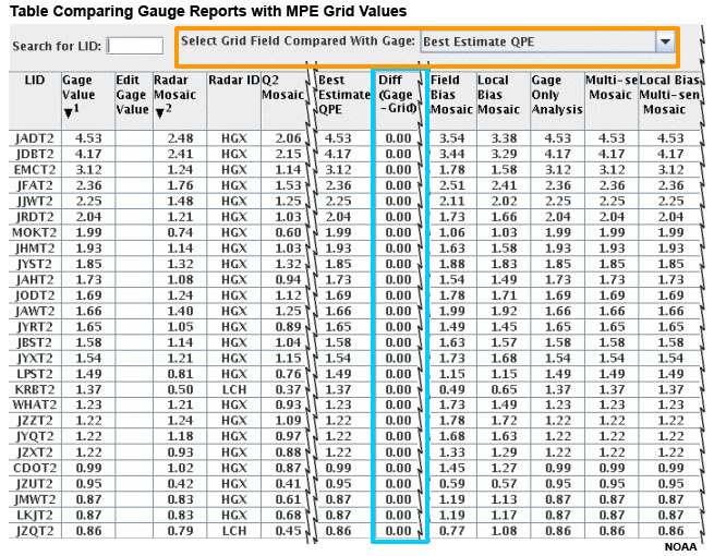
The Gage Table allows the forecaster to interrogate a specific gauge value and compare it with other precipitation estimates.
The left two columns of this table show the gauge identification and its hourly accumulation in inches.
A gauge value can be directly compared with any MPE precipitation field at the grid bin where the gauge is located. This is especially important if the density of the gauge network does not permit good consistency checks with neighboring gauges.
The edit gauge value column allows the user to assign a specific accumulation value to a gauge or set it to missing.
Notice how the gauge values compare with the (2) Radar Mosaic and (3) Q2 Mosaic values. (4) In this case the radar precipitation fields seem low compared to the gauge reports. (5) Bias corrected values show some improvement, assuming the gauge report is correct, but the values are still generally low compared to the gauge reports.
Note that all Multisensor Mosaic values exactly match their corresponding gauge reports. By definition that is what the multisensor fields are supposed to do at the gauge location. Be aware that outside the influence of gauge reports, the multisensor fields may contain large errors due to radar bias. That won’t show up in this table which shows only comparisons at the gauge locations.
- Multisensor mosaic value are supposed to match gauge values at gauge locations
- Multisensor mosaic can have large errors between gauge locations
The blue-highlighted column (below) shows the difference between the gauge report and the MPE grid value at the gauge location. The forecaster can select which MPE grid to compare with. Here we are comparing the Best Estimate QPE with the gauges. Remember that the Best Estimate QPE is whichever MPE grid the forecaster has chosen it to be. In this case, it is the Multisensor Mosaic.
Question
Why are the values all 0.00?
Choose the best answer.
The correct answer is a) By definition the grid and gauge values in a multisensor mosaic should match at gauge locations.
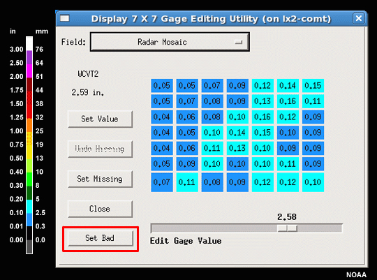
Interrogating Gauge Data: “Display 7X7”
The Display 7X7 is another gauge interrogation tool that allows some important alterations. The gauge identifier (BMDT2) and hourly value is shown in the upper left. This gauge reports 3.66 inches (93 mm).
With the 7X7 display, a forecaster can view the neighborhood of gridded precipitation field values relative to the gauge.
The precipitation field that the gauge is being compared with here is the Radar Mosaic as shown with the Field box, but it can be any MPE Precip Field.
The grid bin that corresponds to the gauge location is in the center and has a value of 2.21inches (56 mm). The display shows the Radar Mosaic values extending 3 bins in each direction.
Notice that within the gauge neighborhood there are no radar mosaic values that match the gauge value. The range of gridded values goes from (8) 0.51-2.48 inches (13-63 mm), all well below the gauge value of 3.66 inches (93 mm).
Question 1 of 2
The gauge is 1.18 inches (30 mm) higher than the highest gridded value in the
gauge neighborhood. What does this mean?
Choose the best answer.
The correct answer is c) Can't tell if it's (a) or (b)
Discrepancies between a gauge and a radar-based precipitation field suggest possible errors in either the gauge report OR the gridded precipitation field. Whether or not the discrepancy is indicative of a bias requires more data, including more reports over time from this gauge, as well as reports from other gauges.
Question 2 of 2
Why do we look at the neighborhood of gridded values instead of just the
grid bin associated with the gauge location?
Choose the best answer.
The correct answer is a) Because there may be precipitation drift between the radar sample and the gauge.
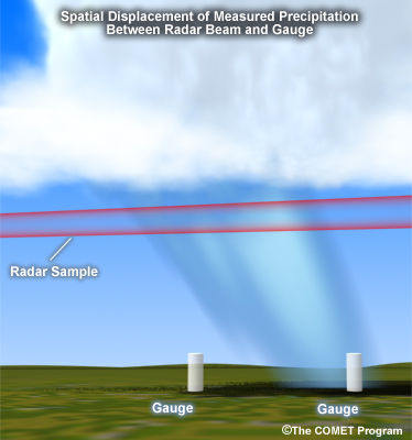
Even if both gauge and radar are functioning perfectly, they should not be expected to always match at the gauge location. There can be a spatial displacement in precipitation between where the radar measures it and where it reaches the ground-based gauge. This displacement is likely to increase as the vertical distance between gauge and radar sample increases with distance from the radar. In addition, the radar may be sampling over a couple square kilometers while the rain gauge aperture may be only 300 square centimeters.
Bad Gauge
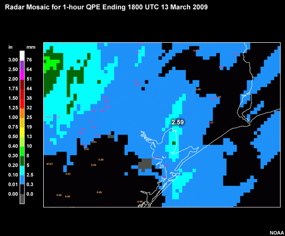
This graphic from 1800 UTC on March 13th 2009 shows MPE’s 1-hour Radar Mosaic zoomed in along the upper Gulf Coast of Texas.
Right here an hourly gauge report shows 2.59 inches (66 mm). This certainly appears to be inconsistent with the radar QPE, especially considering that the radar coverage in this area should be quite good.
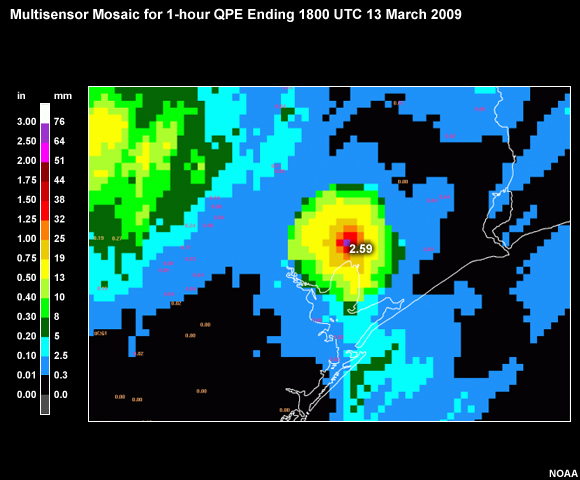
If we look at a Multisensor Mosaic, notice how the gauge location jumps out. Remember that the multisensor fields force the grid value associated with the gauge to the gauge value.
So that explains the one purple grid value associated with the gauge report.
Question
Why does there seem to be a circular area of enhanced values?
Choose the best answer.
The correct answer is d) This reflects one gauge’s radius of influence.
The gauge has a radius of influence where the gauge value is gradually blended back to the radar values.
To remove this potentially bad gauge report let’s use the Display 7X7 function centered on this gauge report with Radar Mosaic as the field. So this bin with a value of 0.14 inch corresponds to this spot on the Radar Mosaic where the gauge is reading 2.59 inches.
Notice how all of the radar values at and within the vicinity of the gauge are much lower than the gauge report.
Among the Display 7X7 functions, the forecaster can set a gauge to “bad” that will remove it from the current and subsequent computations. And like the functions in the Gage Table, the forecaster can change the gauge value with “set value” if that seemed like a more appropriate solution, or set it to “missing”.
Pseudo Gauges
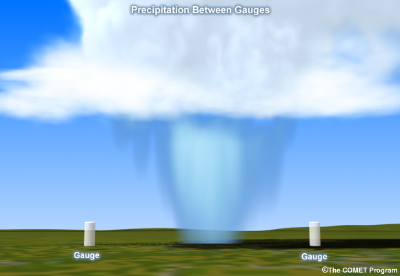
Imagine the following two scenarios. Precipitation is occurring, but most of it is missing the gauge locations.
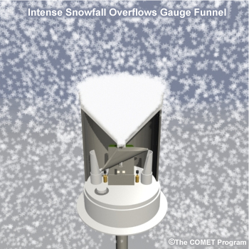
Or, frozen precipitation is occurring and the automated gauges available to MPE are not able to produce accurate liquid equivalent reports. Now consider that in either scenario you may receive a reliable manual report. How can you incorporate this important piece of information?
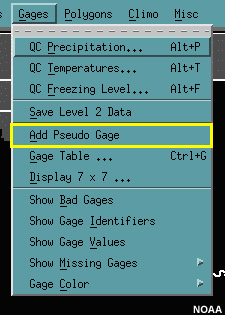
- Pseudo gauge input influences precipitation mosaic for the hour it was created
- Psuedo gauge can be displayed and edited with Gage Table and Display 7x7
This is where adding a pseudo gauge can come in. Available through the “Gages” menu, a pseudo gauge is treated like any other gauge report and can influence the hour’s precipitation fields, including bias computations. The use of a pseudo gauge will only affect the hour in which it was created. It can be altered during that hour with tools like Display 7X7 and the Gage Table.
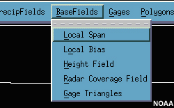
Local Bias Display and Evaluation
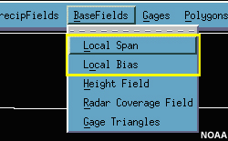
The “Basefields” menu provides access to local bias and radar information. Radar information including beam height and coverage area is accessed through this menu. These aspects of radar data were discussed in Precipitation Estimates 1: Measurement. In this section we will focus on two products associated with the local bias generation. These are the Local Span and the Local Bias.
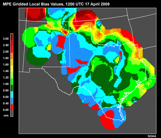
The Local Bias shows the actual value that is applied to gridded radar values for the local bias correction. Values near 1, the green colors, indicate little or no bias. Low values, in blue, are the high bias correction (gauges read lower than the radar). High values, the yellows and oranges, represent the low bias correction (gauges read higher than the radar). Red is used for extreme bias corrections on both ends of the spectrum. Note that on the left side of the area where radar and gauge coverage is sparse, more influence of individual gauges can be seen with the circular patterns.
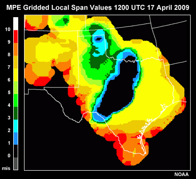
The corresponding Local Span provides information about the time period over which the minimum number of gauge reports was gathered for the bias calculation. The numbers on the color legend represent time periods as shown in the table.
The black in the middle of the Local Span indicates the bias has been updated within the most recent hour.
You can see that this is where the radar accumulation has occurred in the past hour. The blues and greens, categories 1-5, are where rainfall allowed the local bias to update during recent hours. Categories 6-9 indicate where the local bias has not been updated in at least a week. This suggests the bias correction values are rather old, possibly because it has been a dry period, and may not be representative of the current conditions.
Polygon Edits
Precipitation Estimation Process
- Step 1: Differentiate areas of general rain, convective rain, hail, virga, snow, bright band, and radar blockage areas.
- Step 2: Evaluate gauge data and make necessary edits
- Step 3: Re-evaluate precipitation fields after gauge edits
- Step 4: Correct remaining problems, possibly with polygon edits
- Step 5: Adjust precipitation analyses with data that come in later
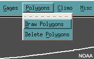
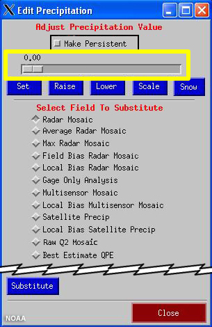
Polygon edits are an important tool for altering data within the MPE precipitation fields. It’s typically a step that comes in after quality control of the gauge data and re-creating the different mosaics. Any problems that still remain may be minimized with polygon edits.
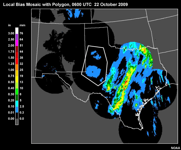
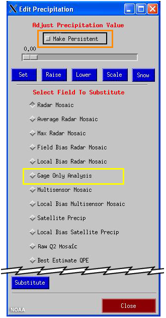
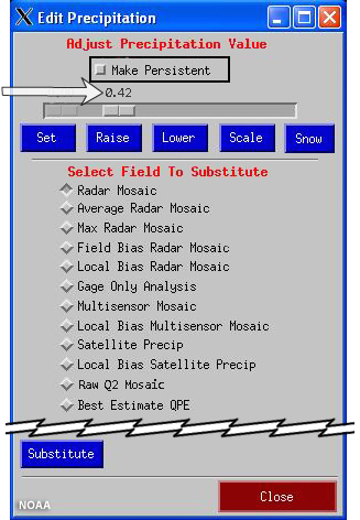
From the polygon edits menu, all of the MPE precip fields are listed under “select field to substitute.” In this case, let’s choose Gage Only Analysis to substitute within the polygon. And if we want this substitution to be used in subsequent hours, we can choose “Make Persistent.” These corrections will continue in subsequent hours until the polygon is deleted.
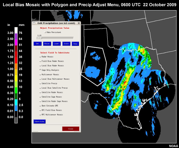
Once we substitute the Gage Only Analysis within the polygon, our Local Bias Mosaic changes from the above, to this, below.
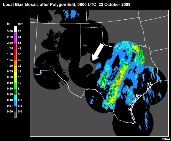
It appears we removed an area of anomalous propagation. The Gage Only Analysis does not cover all grids due to sparse gauge density.
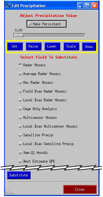
There are several additional ways that the precipitation mosaics can be altered within the polygon. These include setting the area to a given accumulation value; establishing a minimum accumulation value where all values that are lower are raised to that value; establishing a maximum accumulation value where all higher values are lowered; or applying a multiplicative correction to the accumulation values.
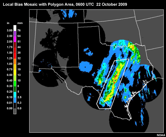
So let’s go back to our original local bias mosaic and draw a polygon around the heavy rain area. If we have reason to believe the estimates are only 50% of what they should be, we can use Scale to apply a multiplicative correction of 2.0 and get this result, below.
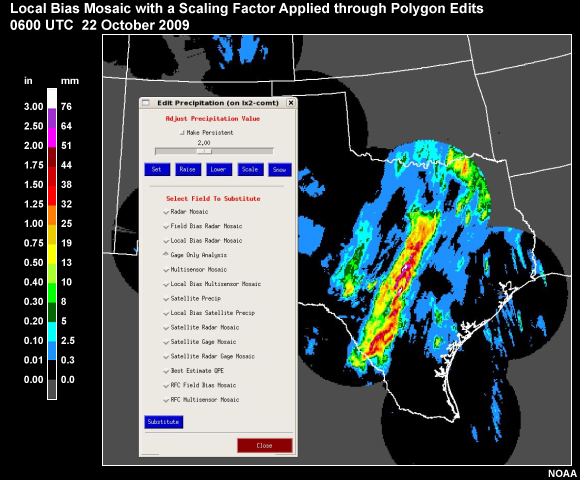
It is essentially like forcing a local bias correction, but the local bias area is the polygon.
Review Questions
Question 1 of 4
A Display 7X7 product helps with comparing a gauge report with MPE gridded values
____.
Choose all that apply.
The correct answers are c) and d)
Question 2 of 4
Which product assists with comparing a gauge report with all MPE gridded fields
in one display?
Choose the best answer.
The correct answer is a) The Gage Table
Question 3 of 4
The Local Span product is useful for _____.
Choose the best answer.
The correct answer is d) determining if a local bias value may be representative
Question 4 of 4
Which edits can be done within a polygon area?
Choose all that apply.
The correct answers are a), b) and d)
Precipitation Estimates Cases
MPE Case Examples:
- Winter Storm: Idaho
- Blocked Radar Sector, New York
- Melting Layer/Bright Band: Ohio
- Bright Band: California
- Convection/Warm Rain: Texas
- Flash Flooding: Georgia
- Long-Duration Accumulation: OHRFC
- Anomalous Propagation: WGRFC
This section includes eight MPE examples. The intent is to provide snapshots of a diverse set of real events. Each case example demonstrates reasonable scientific thought processes and procedures to deal with various phenomena such as: snow water equivalent, bright band, radar coverage, beam blockage, strong convection, warm rain processes, and anomalous propagation.
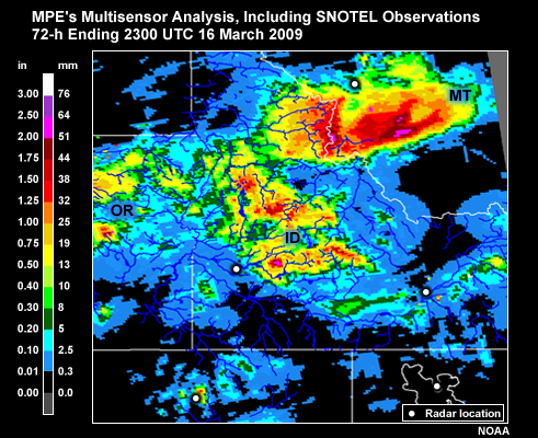
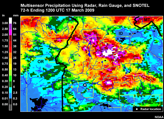
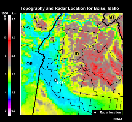
Winter Storm: Idaho
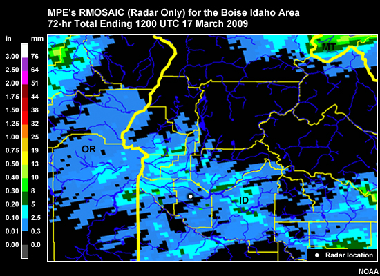
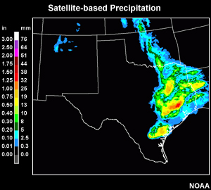
On March 15-17th 2009 a strong winter storm moved across the northern Rockies. The Boise, Idaho county warning area received heavy snow. Here is the MPE Radar Mosaic of liquid equivalent for the 72-h period ending at 1200 UTC March 17th.
Question 1 of 2
What characteristics should you expect with the MPE Radar Mosaic?
Choose all that apply.
The correct answers are b) and c)
Please continue watching the video before answering the next question.
Even close to the radar there is very likely an underestimated liquid equivalent estimate due to the fact the precipitation type is snow.
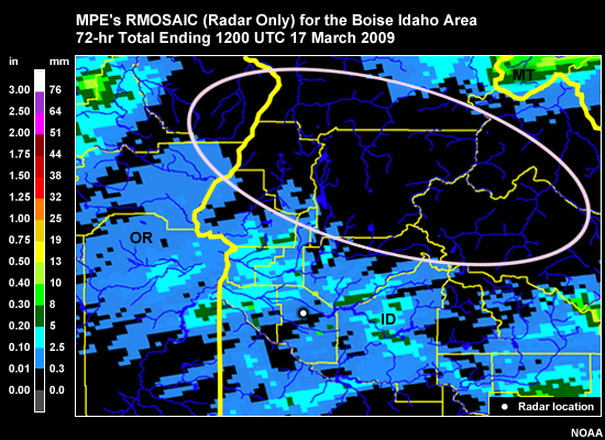
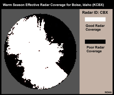
But in this area the lack of precipitation on the Radar Mosaic is due to poor radar coverage.
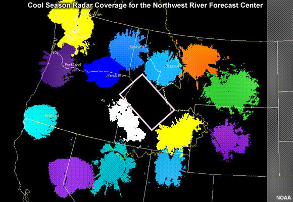
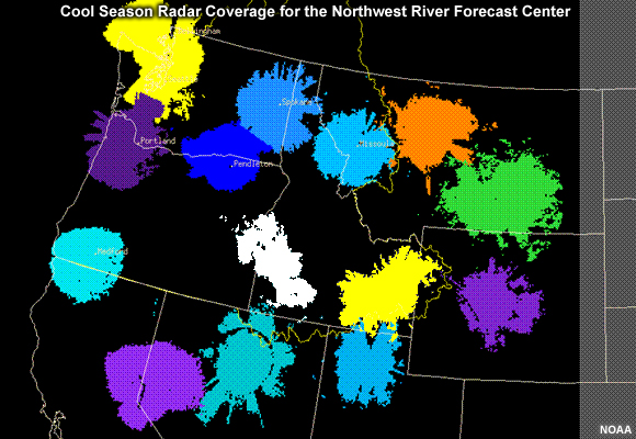
Recall from this radar coverage map shown in Precipitation Estimates, Part 1, that there are large gaps in radar coverage for the Northwest. This includes much of mountainous Idaho northeast of Boise.
Question 2 of 2
What MPE product might be most useful for filling in the area with poor radar
coverage?
Choose the best answer.
The correct answer is d) Multisensor Mosaic
Please continue watching the video for the answer explanation.
Answers a through c are all limited by where the radar is actually detecting precipitation.
So the Multisensor Mosaic is often a good choice where there is poor radar coverage but some reliable ground-based precipitation measurements do exist.
Remember, the gauge information in this product is enhanced by PRISM precipitation climatology.
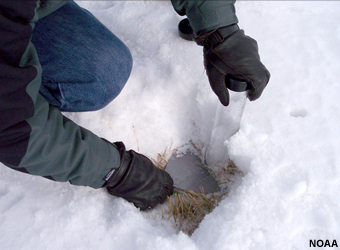
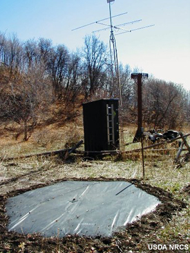
Reliable precipitation measurement is the key. Automated gauges often perform poorly with frozen precipitation. It is important to identify gauge locations with good liquid equivalent measurements.
- Reliable precipitation measurement is key
- Supplement automated gauges with
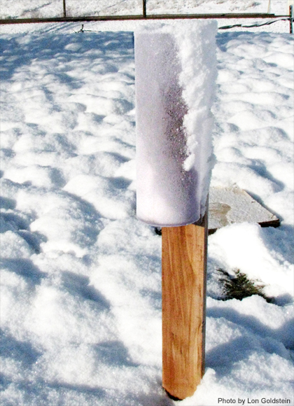
- Snow cores
- Measurement based on weight
This information can be supplemented with snow cores or measurements based on actual snow weight such as those from the SNOTEL sites in the West.
Blocked Radar Sector, New York
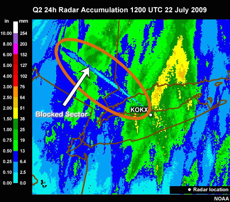
It is common to have a small sector of radar blockage apparent in the radar QPE. One such area extends northwest from the Brookhaven, New York radar and it impacts precipitation estimation in the Hudson Valley. The blocked sector is much smaller than the large areas of poor radar coverage seen in the West, and correcting them in MPE can be different than what we showed in the Boise case.
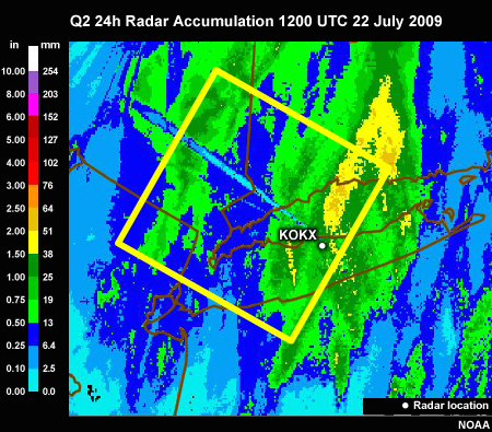
In this case from July 22nd 2009, let’s zoom in to the area within the yellow box and examine the section of poor radar coverage within MPE.
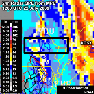
Here is a zoomed in image from the MPE radar mosaic. It has a different colorbar and orientation than the previous image, but you can see the blocked sector in this region.
When the area of blocked radar coverage is this narrow, the forecaster will often choose to fill in the area by estimating the value based on the values seen on either side of the blocked sector.
In this case, polygons were used each hour in the blocked sector. A “set” value was used to specify an accumulation in the polygon based on surrounding values and the movement of the precipitation features.
The polygon feature allows a forecaster to easily assign a value.
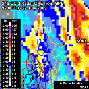
When summed to make a 24-hour total, these accumulations look much more realistic than the one before the polygon edits were made.
Melting Layer/Bright Band: Ohio
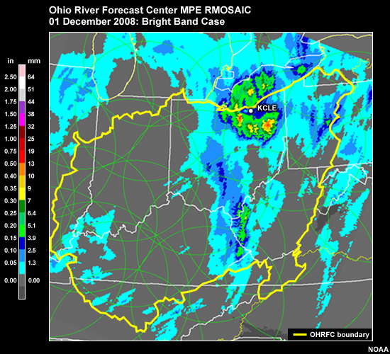
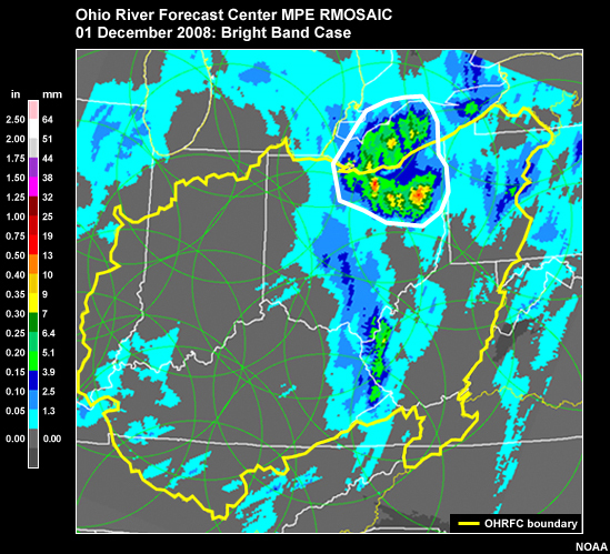
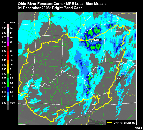
On December 1st 2008 a cold rain fell over part of the Ohio River Forecast Center (OHRFC) area. The Cleveland, Ohio radar showed considerable bright band return where the radar was sampling the melting layer. This resulted in a ring of overestimated radar QPE seen in the Radar Mosaic product.
Question 1 of 2
If the Local Bias Radar Mosaic uses gauges to adjust the radar QPE on the
grid scale, why didn't it make a more complete correction here?
Choose all that apply.
The correct answers are a) and d)
Answer "a" is the most likely reason. Gauge density is not sufficient to represent the small scale nature of bright band within a given hour.
Answer "d" is also correct. Bright band locations often move as the freezing level changes. Therefore a different set of gauges can be impacted from one hour to the next. Answer "c" is not correct because if there is a prominent melting layer aloft, indicated by the bright band, then the surface precipitation should not be snow.
Question 2 of 2
Could polygon edits be used to handle bright band overestimation?
Choose the best answer.
The correct answer is a) Yes
Polygon edits are a common approach to minimizing bright band overestimation.
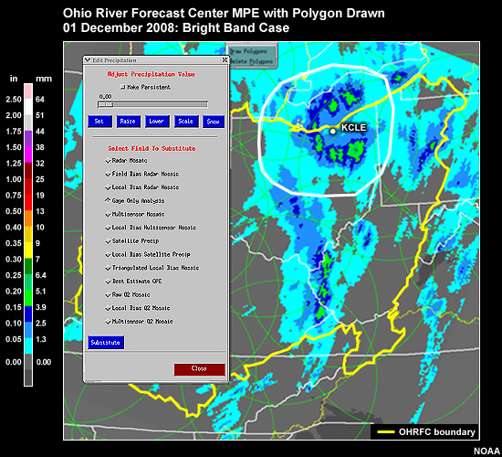
In this case the forecaster drew a polygon around the bright band region.
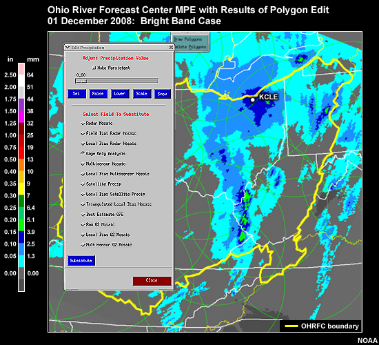
The area within the polygon was replaced with a "Gage-Only Analysis". The result is the removal of the bright band overestimation while preserving the radar QPE structure in areas outside the polygon.
Bright Band: California
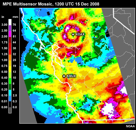
In some cases bright band may be corrected by very dense and reliable rain gauge networks. Here we see an MPE multisensor mosaic. The bright band overestimation around the KMUX radar has been corrected with the multisensor merging due to the very dense gauge network associated with that radar. To the north, there are fewer gauge reports and the bright band associated with the KDAX radar is still clearly visible. Substituting another field, like Gauge Only, via the polygon edit is probably the easiest method for correcting this. That approach was demonstrated in the previous case from Ohio.
Convection/Warm Rain: Texas, Part 1
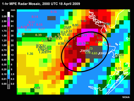
On April 18th 2009 convective rains in southeastern Texas triggered flooding in the Houston area. The MPE Radar Mosaic for the hour ending at 2000 UTC showed some large rainfall amounts. A cluster of hourly gauge reports exceeded three inches (76 mm) and some exceed four inches (104 mm).

Bins near the radar location show missing values.
Question
Look at a handful of hourly gauge reports. How do these compare with the Radar
Mosaic?
Choose the best answer.
The correct answer is c) Gauges significantly higher
In general the gauge reports are reading significantly higher than the radar where the heavier rain is occurring.

In section 3.5 we looked at this gauge report of 3.66 inches (93 mm) using the Display 7X7 tool.
In that section we couldn’t tell if the discrepancy between the gauge’s 3.66 inches and the Radar Mosaic value of 2.21 inches was because the gauge was reading too high or the radar was estimating too low.
Now that we have the context of nearby gauges, it appears that the radar estimate may be biased too low. We can be more confident that this is a good report and should be used in bias and multisensor products.
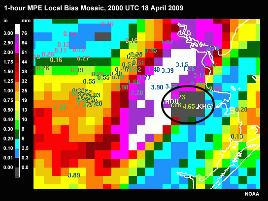
The Local Bias Radar Mosaic makes a significant upward adjustment to the radar accumulation estimates using those gauge reports. This brings the radar QPE much more in line with the gauge reports.
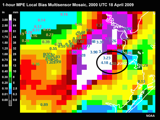
The Local Bias Multisensor Mosaic will force the gridded field to the gauge values at gauge locations and it fills in the missing grids around the radar location using the nearby gauge reports.
Convection/Warm Rain: Texas, Part 2
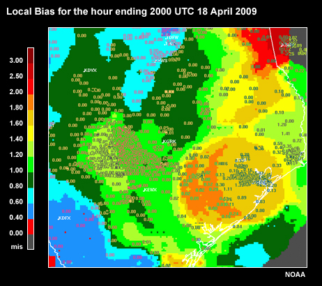
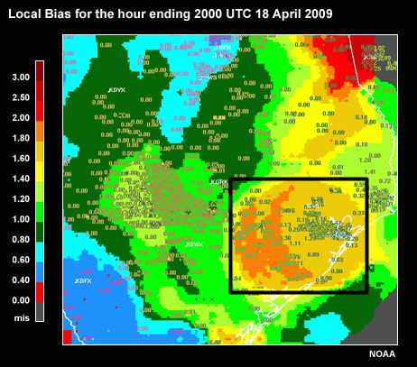
Now we are showing just the local bias correction factor. This is the same location we just examined in the gridded precipitation estimates. Note that the orange colors represent bias correction of 1.60-2.00. This means that the radar is adjusted upward by 60-100% to better match the gauge reports.
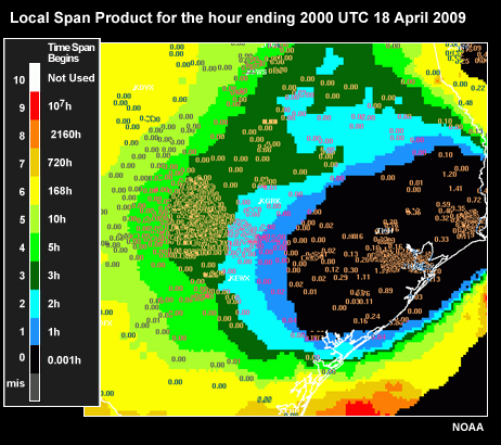
To the left of the box the green colors show bias correction factors closer to 1.0, meaning the gauge-radar pairs showed better agreement. This is where the storm complex was located earlier in the day. Keep in mind that the storms moved eastward toward the Gulf Coast when you look at the local span product.
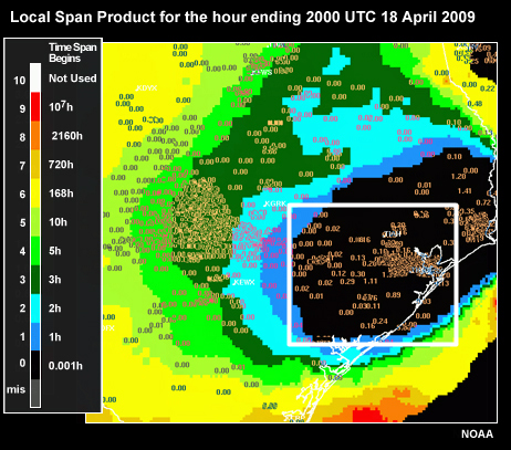
This Local Span graphic shows that the local bias correction factors are for the most recent 3 hours in the black and blue shaded areas. The green indicates that the bias was computed within the last 3-10 hours. The reason in this case being that this is the location of the storms at that time.
So when you combine this information with that from the Local Bias plot, we see that the bias corrections are greater for the more recent calculations.
The bias corrections have changed from ~1.0 to between 1.6 and 2.0 over the last 10 hours.
As the convective storms moved east, they moved into an environment encouraging a deeper warm cloud layer and were fed by greater low-level moisture. The transition to more of a warm rain system was captured by the bias computations.
Remember that this is a gauge dense area where the local bias can keep pace with the storm evolution. In areas that do not have dense gauge coverage, the bias adjustments may lag the trend in the storm characteristics.
This scatterplot shows the gauge reports compared to the MPE Multisensor Mosaic. The diagonal black line indicates where MPE gridded precipitation would be perfectly correlated with gauge reports. The best fit line for this sample is slightly to the right of the diagonal, showing some underestimation by the Multisensor Mosaic, especially at the higher values.
If we overlay the best fit line for the Local Bias Multisensor Mosaic, we see an even better correlation between gauge reports and MPE gridded precipitation.
Gauge reports independent of the MPE 1-hour automated gauge data are used in these verification scatterplots.
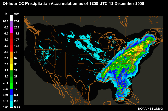
Flash Flooding: Georgia, Part 1
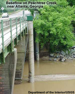
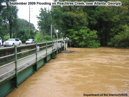
During the period of September 19th thru 22nd 2009, northern Georgia received repeated episodes of intense rainfall. Several notable floods occurred, including Peach Tree Creek in the Atlanta area.
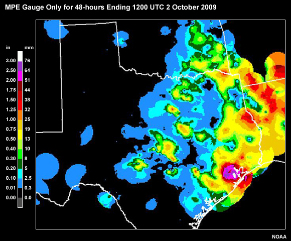
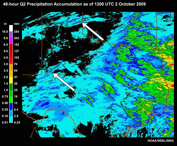
The convection was not associated with hail reports, but did at times contain moderate to high amounts of lightning. Q2 products indicated that for short periods of time there were parts of the convection that took on warm rain characteristics. So the Q2 mosaic is derived using Z-R conversions mainly of convective and stratiform processes, with occasional warm rain enhancement.
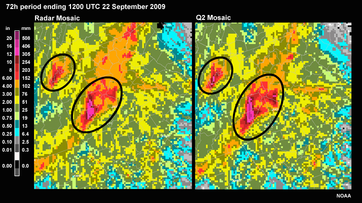
Here are MPE’s Radar Mosaic and the Raw Q2 Mosaic for the 72-hour period ending at 1200 UTC September 22nd. They are similar, but the Raw Q2 Mosaic does show slightly greater values in some of the moderate or heavy rain areas. This is due to the warm rain Z-R conversion being used when appropriate in those areas.
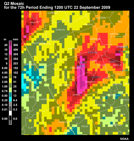
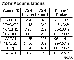
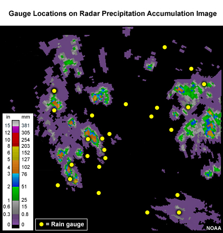
If we zoom in on the Raw Q2 Mosaic, we can see some gauge locations shown in blue. The 72-hour accumulations for these gauge locations are given in the table. The table also shows the ratio of the gauge to the radar values, with the radar values representative of the radar bin directly above the gauge and the 8 nearest neighbor bins. A gauge-over-radar ratio of 100% would be a perfect match. Notice that many of these have 100% within the range of gauge-over-radar ratios. There is a skewing toward ratios greater than 100% indicating the radar may be biased too low.
The Southeast RFC found that the Multisensor Mosaic works best. This image shows the slightly enhanced values in the heavy rain areas with that product. This is the product they chose as MPE’s Best Estimate QPE.
Flash Flooding: Georgia, Part 2
This scatterplot with the MPE accumulation on the Y axis and gauge observations on the X axis is for September 21st. The black diagonal line represents perfect correlation between the gauge reports and the MPE field.
The red dots show the relationship between the rain gauge reports and the Best Estimate QPE, in this case the Multisensor Mosaic. The red diagonal line is the best fit of the red dots. It shows a relatively good fit, with some underestimation of the higher amounts as seen by the best fit line being below the diagonal.
We can also do this for the Raw Q2 Mosaic and the Radar Mosaic. We didn’t include the points to avoid clutter, but the best fit lines for those fields can be compared with the Best Estimate QPE. The Raw Q2 Mosaic is represented by the pink line and shows a little more underestimation by the radar. The Radar Mosaic is represented by the orange line. Although this is not a terrible fit, it does show that without either the Z-R adjustment in Q2 or the gauge blending and field bias correction in MPE’s Multisensor mosaic, there is greater underestimation in the radar-based QPE.
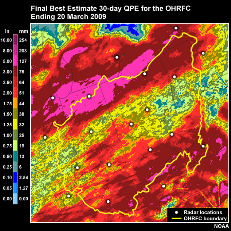
Long-Duration Accumulation: OHRFC
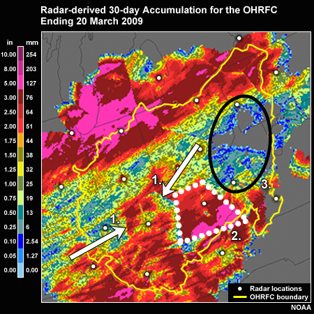
Sometimes it helps to look at long-duration QPE to identify problem areas and calibration differences between radars. Even in regions without abrupt terrain features, radar artifacts can appear in the long-term accumulations.
This image shows the 30-day radar accumulation from MPE. (1) You can see discrepancies and the boundaries between radar coverage areas. (2) The Jackson, Kentucky radar appears to be calibrated differently than surrounding radars. (3) There is an area with no radar QPE between Pittsburgh and Charleston that is not fully supported by ground reports.
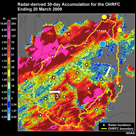
(1) The radar at Pittsburgh appears to have lower magnitudes than those (2) at Buffalo and State College. (3) You can also see blocked sectors from the Louisville and Charleston locations.
In this 30-day accumulation for the same period, the quality has been improved within the Ohio River Forecast Center area through the use of the tools and datasets in MPE.
Anomalous Propagation: WGRFC
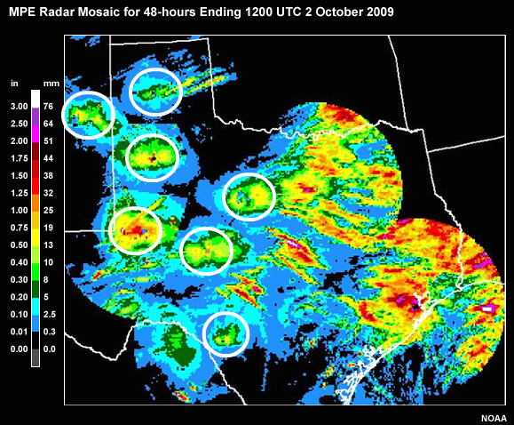
In this MPE Radar Mosaic image we are looking at a 48-hour accumulation. There was little or no rain in western Texas, but reflection of ground targets from anomalous propagation shows up as significant accumulation around many of the radar sites.
Within these areas there are also some narrow bands of significant precipitation.
The local bias product does little to help because there are very few non-zero gauge reports and it preserves the structure of the radar fields. Here we show the Multisensor Mosaic and we still see considerable anomalous propagation signatures. This is because there aren’t enough gauges to correct the problem.
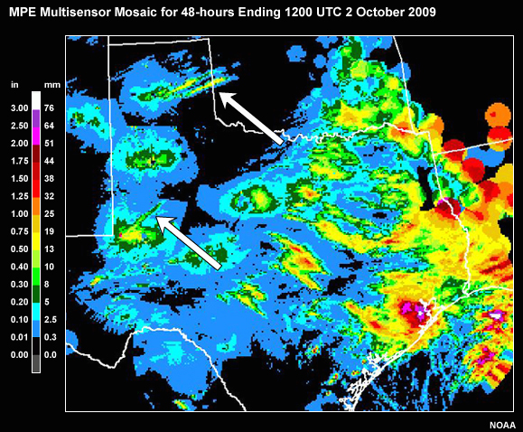
A common option is to use polygons to substitute the Gage Only Analysis in areas of anomalous propagation. However when you have localized precipitation mixed in, the risk is that the Gage Only Analysis will remove the real precipitation along with the anomalous propagation.
That is what we see in this Gage Only Analysis. Some of the localized precipitation bands observed by the radar are gone because the gauges did not sample them.
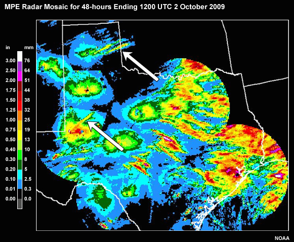
The Raw Q2 Mosaic provides another option that is often good at removing anomalous propagation, while preserving the coverage and structure of any real precipitation observed by the radar. Note that these narrow bands of accumulation absent in the Gage Only Analysis, are back in the Raw Q2 Mosaic.
Summary
The Multisensor Precipitation Estimator (MPE) uses information from gauges, radar, and/or satellite to produce gridded mosaics of observed precipitation, often referred to as QPE. A variety of products and editing tools within MPE allow the forecaster to base the best QPE on one sensor or some optimal combination of information from multiple sensors. These gridded QPE products serve as important inputs to hydrologic models.
Key Points
Gridded QPE from each measuring platform is available separately through MPE. There may be multiple ways to display radar QPE. Rain gauge data are available as climate-enhanced gridded QPE or as data plots.
MPE also provides many QPE choices that use information from multiple sources. There are two primary combination techniques that use rain gauge data to enhance radar QPE.
One technique uses gauge data to determine if a bias exists.
The second basic technique is to blend one of the bias-adjusted radar QPE products with a rain gauge analysis to get a multisensor mosaic.
Comparison of Multisensor Products vs. Bias-adjusted Products:
| Multisensor Products | Bias-adjusted Products |
|---|---|
| Can fill in areas with missing radar QPE | Only values where radar QPE exists |
| Grid box value at gauge location equals gauge value | Grid box value at gauge location does not always equal gauge value |
| Spatial detail and relative values of radar QPE may be altered | Spatial detail and relative values of radar QPE preserved |
| Performed with very few gauges | Minimum number of gauge-radar pairs required |
The bias-adjustment procedures preserve the spatial pattern and relative values of the radar QPE. A minimum number of gauge-radar pairs is needed to compute a bias.
The multisensor products do not necessarily preserve the radar pattern and do not have a minimum number of gauges required. An important strength of the multisensor approach is that the gauge data can be used to fill in areas of poor radar coverage. The multisensor products are typically regarded as the final QPE product.
There are many combinations of the different sensor information within MPE products. The product that performs best may vary with season, location, and even from event to event.
The Best Estimate QPE can be set to whichever QPE product is considered optimal for the time, location, or conditions. In any given hour the forecaster can make QC decisions and edits to any Precipitation Field and save it as the Best Estimate QPE. The Best Estimate QPE is used in hydrologic models and in RFC mosaics that are used to make the national precipitation mosaic.
Methodology
Step 1: Differentiate areas of general rain, convective rain, hail, virga, snow, bright band, and radar blockage areas.
Step 2: Evaluate gauge data and make necessary edits
Step 3: Re-evaluate precipitation fields after gauge edits
Step 4: Correct remaining problems, possibly with polygon edits
Step 5: Adjust precipitation analyses with data that comes in later (i.e. additional gauge data, snow cores, SNOTEL data, NOHRSC data…)
There are different uses for MPE within the analysis and forecast process. A common process is shown in this 5-step sequence. The process typically involves identifying the characteristics of the precipitation, evaluating and possibly editing the gauge data, and then re-evaluating the MPE guidance with the QC’d gauge information. The gauge QC step is very important because of how the gauges are used as ground truth measurement in many of the MPE products.
If problems remain in the QPE, it may be useful to use polygon edits. In addition, some products are adjusted later with additional data from alternate sources.
References
Curtis, David C., and R. Burnash, 1996: Inadvertent rain gauge inconsistencies and their effect on hydrologic analysis. Proceedings: 1996 California-Nevada ALERT Users Group Conference, Ventura, CA, May 15-17, 1996.
DiLuzio, M., G.L. Johnson, C. Daly, J.K. Eischeid, and J.G. Arnold, 2008: Constructing retrospective gridded daily precipitation and temperature datasets for the conterminous United States. Journal of Applied Meteorology and Climatology, 47: 475-497.
Guo, James C. Y., B. Urbonas, and K. Stewart, 2001: Rain catch under wind and vegetal cover effects. Journal of Hydrologic Engineering, Vol. 6, 29-33.
Sieck, Lisa C., S. Burgess, and M. Steiner, 2007: Challenges in obtaining reliable measurements of point rainfall. AGU, Water Resources Research, Vol. 43
Vasiloff, Steven V., D. J. Seo, K. Howard, J. Zhang, D. Kitzmiller, M. Mullusky, W. Krajewski, E. Brandes, R. Rabin, D. Berkowitz, H. Brooks, J. McGinley, R. Kuligowski, and B. Brown, 2007: Improving QPE and very short term QPF: an initiative for a community-wide integrated approach. Bulletin of the American Meteorological Society, Vol. 88, Issue 12, 1899-1911.
More recently precipitation estimates are performed by the Multi Radar Multi Sensor (MRMS) Program:
https://www.nssl.noaa.gov/projects/mrms/
PRISM products and presentations from the PRISM group at Oregon State
University
http://www.prism.oregonstate.edu/
Contributors
COMET Sponsors
The COMET® Program is sponsored by NOAA National Weather Service (NWS), with additional funding by:
- Air Force Weather (AFW)
- Australian Bureau of Meteorology (BoM)
- European Organisation for the Exploitation of Meteorological Satellites (EUMETSAT)
- Meteorological Service of Canada (MSC)
- National Environmental Education Foundation (NEEF)
- National Polar-orbiting Operational Environmental Satellite System (NPOESS)
- NOAA National Environmental Satellite, Data and Information Service (NESDIS)
- Naval Meteorology and Oceanography Command (NMOC)
Project Contributors
Senior Project Manager
- Wendy Abshire — UCAR/COMET
Principal Scientist
- Matthew Kelsch — UCAR/COMET
Project Leads
- Lon Goldstein — UCAR/COMET
- Matthew Kelsch — UCAR/COMET
Instructional Design
- Lon Goldstein — UCAR/COMET
Additional Science Contributors
- Greg Shelton — NWS
- Jay Breidenbach — NWS
- Paul Tilles — NWS
Graphics/Interface Design
- Steve Deyo — UCAR/COMET
- Brannan McGill — UCAR/COMET
- Lon Goldstein — UCAR/COMET
Multimedia Authoring
- Carl Whitehurst— UCAR/COMET
Audio Editing/Production
- Seth Lamos— UCAR/COMET
Audio Narration
- Matthew Kelsch — UCAR/COMET
COMET HTML Integration Team 2020
- Tim Alberta — Project Manager
- Dolores Kiessling — Project Lead
- Steve Deyo — Graphic Artist
- Gary Pacheco — Lead Web Developer
- David Russi — Translations
- Gretchen Throop Williams — Web Developer
- Tyler Winstead — Web Developer
COMET Staff, January 2010
Director
- Dr. Timothy Spangler
Deputy Director
- Dr. Joe Lamos
Administration
- Elizabeth Lessard, Administration and Business Manager
- Lorrie Alberta
- Michelle Harrison
- Hildy Kane
- Ellen Martinez
Hardware/Software Support and Programming
- Tim Alberta, Group Manager
- Bob Bubon
- James Hamm
- Ken Kim
- Mark Mulholland
- Wade Pentz, Student
- Malte Winkler
Instructional Designers
- Dr. Patrick Parrish, Senior Project Manager
- Dr. Alan Bol
- Maria Frostic
- Lon Goldstein
- Bryan Guarente
- Dr. Vickie Johnson
- Tsvetomir Ross-Lazarov
- Marianne Weingroff
Media Production Group
- Bruce Muller, Group Manager
- Steve Deyo
- Seth Lamos
- Brannan McGill
- Dan Riter
- Carl Whitehurst
Meteorologists/Scientists
- Dr. Greg Byrd, Senior Project Manager
- Wendy Schreiber-Abshire, Senior Project Manager
- Dr. William Bua
- Patrick Dills
- Dr. Stephen Jascourt
- Matthew Kelsch
- Dolores Kiessling
- Dr. Arlene Laing
- Dave Linder
- Dr. Elizabeth Mulvihill Page
- Amy Stevermer
- Warren Rodie
Science Writer
- Jennifer Frazer
Spanish Translations
- David Russi
NOAA/National Weather Service - Forecast Decision Training Branch
- Anthony Mostek, Branch Chief
- Dr. Richard Koehler, Hydrology Training Lead
- Brian Motta, IFPS Training
- Dr. Robert Rozumalski, SOO Science and Training Resource (SOO/STRC) Coordinator
- Ross Van Til, Meteorologist
- Shannon White, AWIPS Training
Meteorological Service of Canada Visiting Meteorologists
- Phil Chadwick