Produced by The COMET® Program
Mystery: Our Fascination with the Aurora
Mystery
“The most beautiful experience we can have is the mysterious. It is the fundamental emotion which stands at the cradle of true art and true science. Whoever does not know it and can no longer wonder, no longer marvel, is as good as dead, and his eyes are dimmed.”—Albert Einstein 1
“I will show you, whether you like it or not, that physics is beautiful. And you may even start to like it.”—Walter Lewin 2

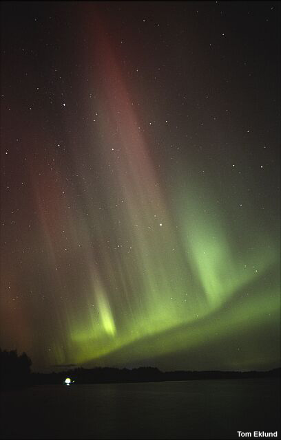
Long before quantum physics, long before astronomy; prior to any concept of electromagnetism, mechanics, science, or mathematics; long before our invention of tools and language, in a primeval time that was measured only by season, sunset, moon phase and heartbeat, our imagination took flight in the dance of these lights. They speak to us across the ages, of stories long forgotten, of heart’s blood stirred in winter darkness, long before the dawn of human mind.
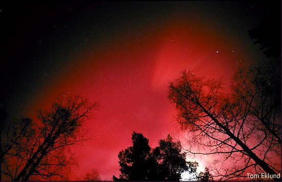
What are these lights? Where do they come from—the Sun, the Earth, the stars? Why do they descend upon us? What gives them such unearthly colors?
The answers are many, reflecting the multiple dimensions of human expression: physical, mathematical, historical, psychological, poetic, and mythic. Our focus, in this learning module, is on the physics of the aurora. You will learn about the systems and processes through which the Earth’s magnetic field and upper atmosphere capture the solar wind to light up the polar sky.
But, before delving into the science of the aurora, take a moment to consider some mythic and
historical perspectives on these amazing phenomena. Let this introduction serve to whet your
appetite and sharpen your interest in exploring the many mysteries of the aurora.
references
- Einstein, A., The World as I See It, translated by A. Harris, Watts and Company, London, 1940.
- Massachusetts Institute of Technology online course materials for Physics 8.02.
Lore
In the lore of many cultures, the aurora are ghosts and spirits at sport or war in the heavens. Inuit legends describe them as “…the souls of the dead...playing football with a walrus head” or the spirits of stillborn children, who “play at ball with their afterbirth.” 1
Longfellow retold Native American legends in The Song of Hiawatha, wherein the young hero was
“Shown the Death-Dance of the spirits,
Warriors with their plumes and war-clubs,
Flaring far away to northward
In the frosty nights of Winter;
Shown the broad white road in heaven,
Pathway of the ghosts, the shadows,
Running straight across the heavens,
Crowded with the ghosts, the shadows.” 2

Russian Lapps explained red aurora to be the blood spilt by murderous spirits, while Scottish tales tell of clan feuds fought by “merry dancers.”

When the Valkyries of Norse mythology rode forth to choose the battle slain, their armor “…shed a strange flickering light which flashed over the northern skies.” 3 Such legends seem to echo biblical accounts of “horsemen running in the air, in cloth of gold, and armed with lances like a band of soldiers.” 4
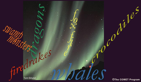
Other legends attribute the aurora to mythic beasts such as dragons, firedrakes, giant arctic whales or crocodiles, swamp monsters, and Repu, the fox of Finnish lore, whose luminous fur emits fox fire.
references
- Nansen, F., Eskimo Life, Longmans, Green and Company, London. 1893; cited in Eather, R. H. Majestic Lights: The Aurora in Science, History and the Arts. Washington D.C.: American Geophysical Union, 1980, p. 110.
- Longfellow, H.W., The Song of Hiawatha, Tickner and Fields, Boston, 1885.
- Leach, M. (Ed.), Standard Dictionary of Folklore, Mythology and Legend, Funk and Wagnals, New York, 1949.; cited in Majestic Lights: The Aurora in Science, History and the Arts, p. 114.
- Maccabees II (5:2)
Early Science
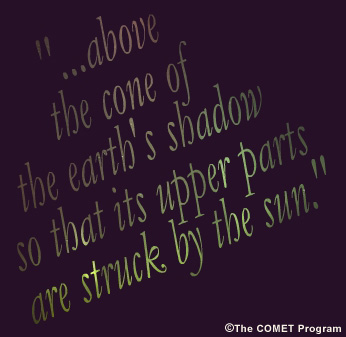
Over the ages, the aurora have sparked the curiosity of many philosophers and scientists. Aristotle described their “chasms, trenches, and blood-red colors.” 1 Seneca described how “the heavens seem to open up and to vomit flames which before were hidden…” 2 Galileo, who named them the aurora borealis, theorized about their formation when portions of the atmosphere rise “… above the cone of the Earth’s shadow so that its upper parts are struck by the sun.” 3
Edmund Halley developed several aurora hypotheses, including a theory that “magnetical effluvia, whose atoms freely permeate the pores of most solid bodies” could travel through the Earth, sometimes carrying “with them out of the Bowels of the Earth a sort of atom proper to produce Light in the Ether.” 4

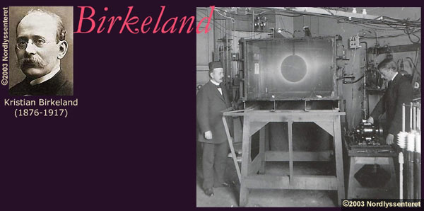
The lengthy list of auroral theorists also includes such famous names as Kepler, Euler, Descartes, Celsius, Cavendish, Franklin, Volta, Gauss, Angström, Birkeland, Störmer, Chapman, Ferraro, Alfvén, and James Van Allen.

Birkeland, in particular, devoted tremendous time, energy, and imagination to the study of the aurora. His Arctic expeditions and observing stations enabled the first accurate measurements of auroral height and intense atmospheric currents generated during magnetic storms. Birkeland also attempted to create aurora in his laboratory. Donning a fez (for protection) he shot cathode rays at his “terella,” a phosphor-coated sphere that encased a 20,000 volt electromagnet. 5, 6
references
- Aristotle, Meteorologica, trans. E.W. Webster
- Seneca, Naturales Quaestiones, Book 1, translated by T.H. Corcoran, Harvard University Press, Cambridge, MA., 1972; cited in Majestic Lights: The Aurora in Science, History and the Arts, p. 39.
- Galileo, G., Le Opere di Gilileo Galilei, 2nd ed., Edizione Nazionale, Florence, 1929-1939; cited in Majestic Lights: The Aurora in Science, History and the Arts, p. 48.
- Halley, E., An account of the late surprising appearance of the lights seen in the air, Phil. Trans. Roy. Soc., 29, 406, 1716; cited in Majestic Lights: The Aurora in Science, History and the Arts, pp 50-52.
- Carlowicz, M. and Lopez, R. (2002), Storms from the Sun. Washington DC: Joseph Henry Press, pp. 64-66.
- Friedman, H. (1986), Sun and Earth. New York: Scientific American Books, pp. 165-166.
links
- Solar Physics Historical Timeline (NCAR/HAO)
Preview
Having considered some of the lore and history of the aurora, we will now turn our attention to the physics of the aurora. In the following sections of this module, you will become acquainted with the electrodynamical and photochemical processes at play in an auroral display. You will learn about the Earth’s magnetic field and its interconnections with the solar wind and atmospheric electric currents. You will examine the charged and neutral dimensions of the Earth’s upper atmosphere, learning how thermal, magnetic and electrical forces stir and shape it. You will also become familiar with the particle sources of auroral emissions and how they are generated.
You can explore the content of this module at three levels of depth.
Overview
Overview pages provide a general introduction to the full range of topics.
Details
Details pages offer elaborations, allowing you to extend your knowledge.
In-depth Topics
In-depth topics present the mathematical and theoretical underpinnings of the physics presented in this module.
Whatever path you take through this module, we invite you to enjoy the journey. May it enrich your understanding and inspire you to further studies of this fascinating domain in the future.
Magnetosphere: Earth's Magnetic Shield Against the Solar Wind
Structure & Formation
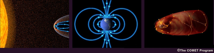
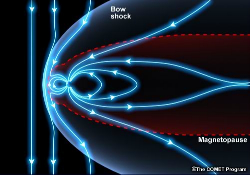
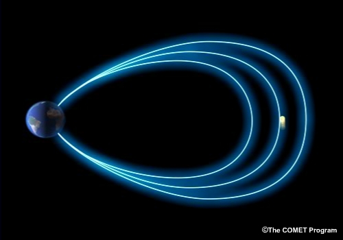
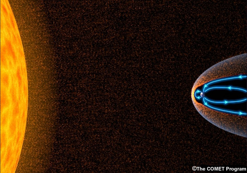
Close to its surface, the earth’s magnetic field is nearly a dipole field, with the dipole axis tilted almost 12° away from the earth’s rotation axis.

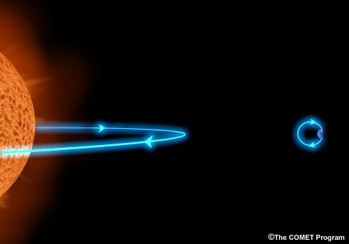
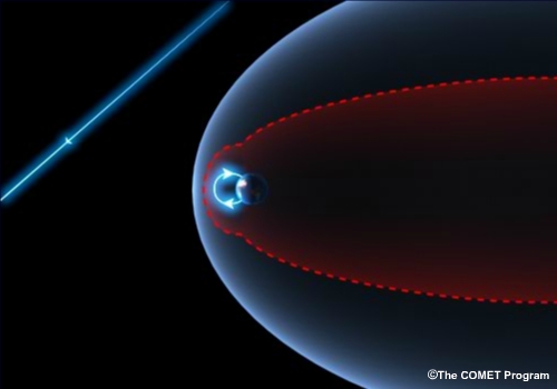
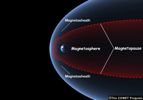
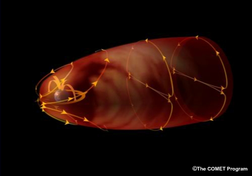
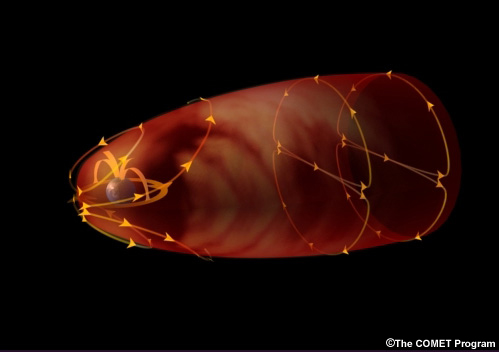
Far from the earth, though, the magnetic field is strongly influenced by the solar wind, a highly supersonic plasma flow emanating from the sun. Because of its high electrical conductivity, the solar wind sees the earth’s magnetic field as a blunt object around which it must flow (much like air flowing past a supersonic jet plane), and it shapes the field into what we call the magnetosphere.
The solar wind makes a sudden transition from supersonic to subsonic flow as it passes
through a bow shock (like the bow wave in front of a boat), and it compresses the magnetic
field on the earth’s day side, while dragging the field into a comet-like tail on the
earth’s night side.
All these effects are illustrated in the following numerical simulation of the solar wind impacting a planetary dipole magnetic field.
Explore More
Click to view the full simulationExplore More
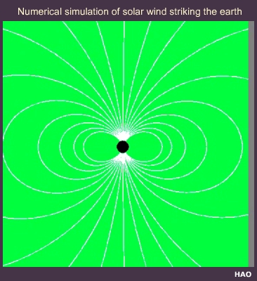
This simulation, developed by Mike Wiltberger and Charles Goodrich, was created
by imposing a solar wind with no magnetic field and a constant solar wind
density against the dipole field of the Earth.
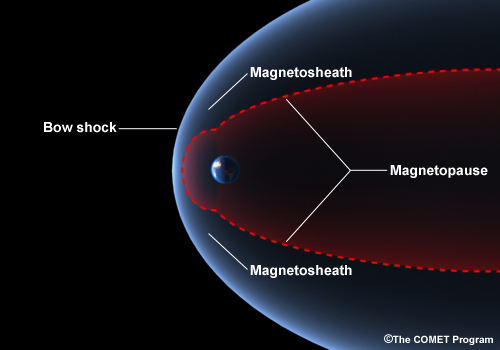
This simulation clearly
shows the compression of the magnetic field on the dayside, stretching of the
field on the nightside, as well as the formation of the bow shock,
magnetosheath, and magnetopause.
Related In-depth topic:
Frozen-Field
Theorem
Magnetic Convection
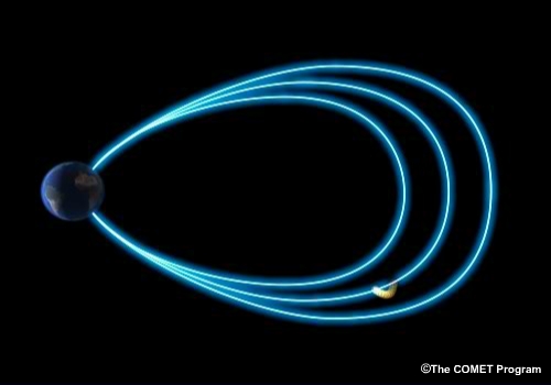
As the solar wind flows past the magnetosphere, it exerts a tangential stress on the magnetopause boundary, driving large-scale plasma convection in the magnetosphere.
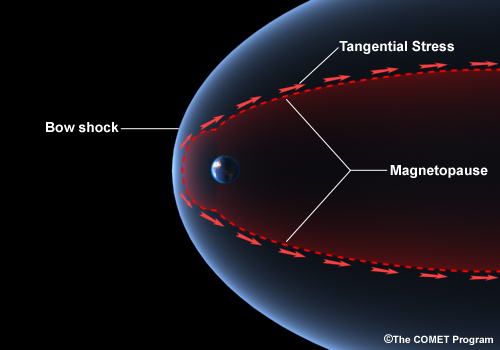
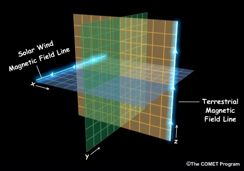
The tangential stress arises primarily from magnetic field line reconnection at the dayside magnetopause. The resulting reconnection-driven convection can be visualized by following a southward solar wind magnetic field line that reconnects with a northward terrestrial field line at the dayside magnetopause.
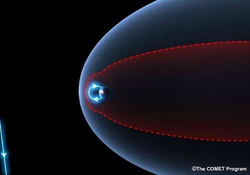
The two new open field lines (connecting the Earth to the solar wind) are carried over the poles, where they again reconnect in the tail of the magnetosphere, forming a newly closed terrestrial field line and a solar wind field line. The newly closed field line moves towards the Earth, then around the Earth and out to the dayside magnetopause, where the process begins anew.
This animation shows reconnection for only a single set of field lines, but the process occurs over a continuum of field lines in the real magnetosphere.
Explore More
Click to view the full reconnection animationDig Deeper
Magnetic
Force
Frozen-Field
Theorem
Magnetic Reconnection
We use the terms breaking and reconnecting to describe magnetic field-line reconnection, but these are approximate descriptions of what happens in the reconnection region, where the Frozen Field Theorem breaks down, and magnetic field lines lose their identity.
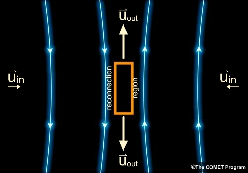
When the magnetic fields in two adjacent regions are anti-parallel, the oppositely- directed field lines move slowly into the reconnection region. Here, they lose their identity, and we say that they break, reconnect, and are rapidly expelled by the magnetic tension force. In this example, all field lines lie in the x-z plane. This type of anti-parallel reconnection was illustrated on the preceding pages at the dayside magnetopause and in the magnetotail.
In reality, the average solar wind magnetic field is approximately perpendicular to the terrestrial magnetic field, but reconnection can still take place. Field lines entering the reconnection region from the left lie in the x-y plane, those entering from the right lie in the x-z plane, and those exiting the reconnection region lie in the y-z plane. The tension force expelling the field from the reconnection region has components in the y direction above the y-z plane and in the negative y direction below the y-z plane.
Related In-Depth Topics:
Magnetic
Force
Frozen-Field
Theorem
Reconnection-Driven Convection
Magnetic reconnection in the magnetosphere drives convection in the Earth's ionosphere. Let’s examine patterns of reconnection and convection for three different solar wind magnetic fields.
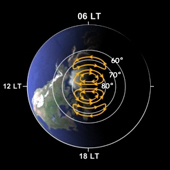
A southward solar wind magnetic field produces anti-parallel reconnection at the dayside magnetopause. In the polar cap ionosphere, magnetic field lines are open to the solar wind, and ionospheric flow from local noon to local midnight corresponds to magnetospheric flow of open field lines from the dayside magnetopause into the magnetotail.
Recall that after magnetotail reconnection, magnetospheric field lines approach the Earth, then swing around it out to the dayside magnetopause. These motions induce ionospheric flow toward lower latitudes near local midnight, with return flow toward the day side at these lower latitudes, and finally flow toward the poles near local noon.
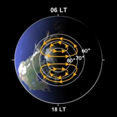
When the solar wind magnetic field is oriented northward, reconnection does not occur on the dayside magnetopause. Instead, anti-parallel reconnection occurs just tailward of the Earth, inducing a very different ionospheric convection pattern.

In this case, there is flow across the poles toward the Sun, with return flow going to lower latitudes on the day side, and turning back around toward the night side. This circulation exists only at very high geomagnetic latitudes (above about 80º); at lower latitudes there is a weak form of the ionospheric convection pattern that we saw for a southward solar wind magnetic field.
When the solar wind magnetic field is oriented eastward (from dawn to dusk), dayside reconnection produces a component of the plasma flow toward the dawn side over the Northern Hemisphere polar cap and a component of the flow toward the dusk side over the Southern Hemisphere polar cap.
These patterns are reversed with westward (dusk to dawn) solar wind magnetic fields.
Explore More
Southward
Northward
Eastward
Answer This
Question
Can you match the IMF configurations with the
corresponding Northern Hemisphere ionospheric convection patterns?
(Choose a pattern from each dropdown box, then click done.)
Pattern A
Pattern B

Pattern C
Pattern D

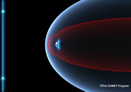
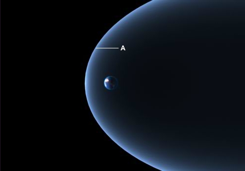
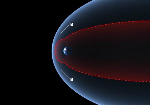
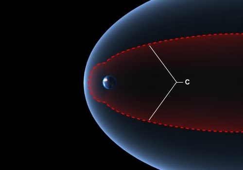
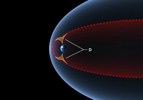
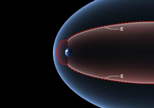
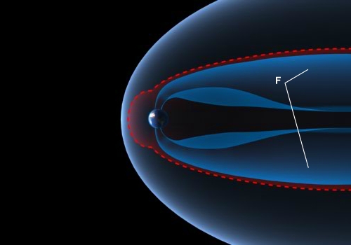
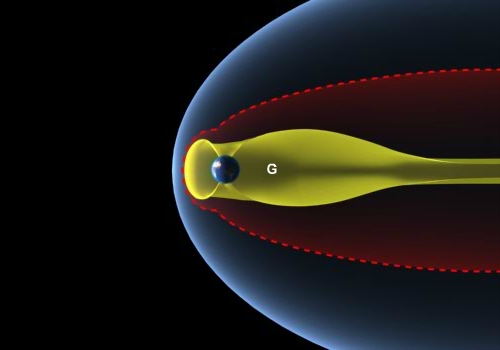
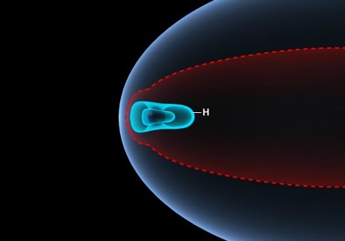
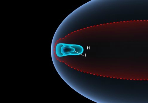
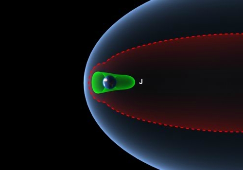
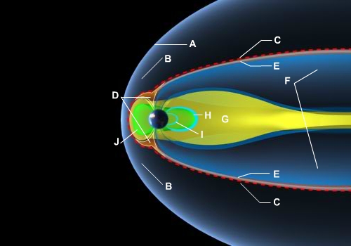
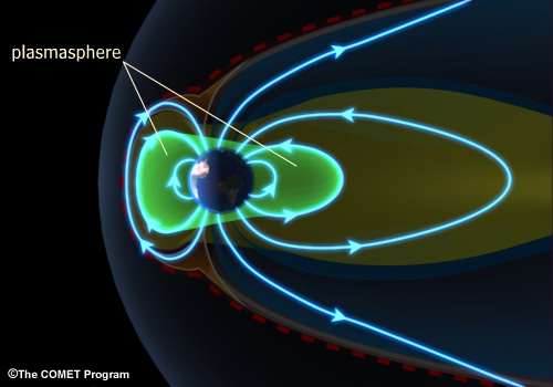
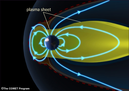
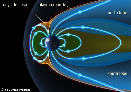
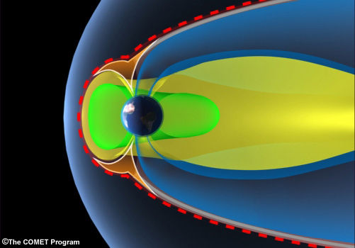
Regions
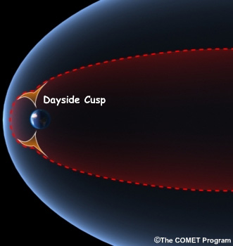
When dayside reconnection opens magnetic field lines at the magnetopause, hot, subsonic solar wind plasma in the magnetosheath gains direct access to the magnetosphere, producing the dayside cusp and plasma mantle. As open field lines are dragged into the magnetotail, they relinquish some of their hot solar wind plasma and fill with cool ionospheric plasma, producing a low density mixed plasma in the magnetotail lobes.
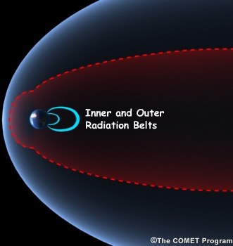
Upon magnetotail reconnection, earthward-bound closed field lines compress the plasma forming the plasma sheet. Particle energies in the plasma sheet increase through compression as the field lines approach the Earth, and the energetic particles begin to drift around the Earth (ions to the west and electrons to the east), forming the outer radiation belt and extending the plasma sheet to the dayside magnetosphere. The inner radiation belt, produced by cosmic rays, lies inside the plasmasphere, which rotates with the Earth's atmosphere, and does not take part in large-scale magnetospheric convection.
Explore More
Answer This
Question
Identify the main regions of the earth's magnetosphere.
(Use the dropdown boxes to choose the names and figures
corresponding to each figure. Click A-J to see the figures labeled. When
finished, click Done.)
Related In-Depth Topics:
Charged Particle
Motion
Magnetosphere-Ionosphere Current System
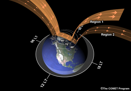
Because the magnetopause boundary separates a region of relatively strong magnetic field (the magnetosphere) from a region of relatively weak magnetic field (the magnetosheath), the boundary must carry a surface current to maintain force balance across the boundary. This magnetopause current flows differently on the day side and night side of the earth.
The magnetopause current encircling the two magnetotail lobes closes through the middle of the tail in a neutral sheet current that separates the oppositely directed magnetic fields above and below. Part of the dayside magnetopause current closes on the magnetopause and part closes via Region 1 field-classed currents in the ionosphere.
The ring current lies in the inner part of the plasma sheet, where ions and electrons drift in opposite directions around the earth. This ring current encircles the earth and is not uniform, with the stronger current flowing on the night side of the earth. The ring current closes partially within the magnetosphere and partially through ionospheric currents via Region 2 field-classed currents.
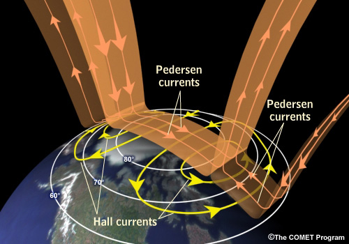
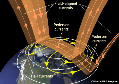
Ionospheric closing currents comprise both Hall and Pedersen currents. Hall currents flow perpendicular to both fields, while Pedersen currents flow parallel to the electric field and perpendicular to the magnetic field. If the ionospheric conductivity were uniform, then the closing would be accomplished solely by Pedersen currents, but conductivity gradients do generally exist, so there is a closing contribution from Hall currents.
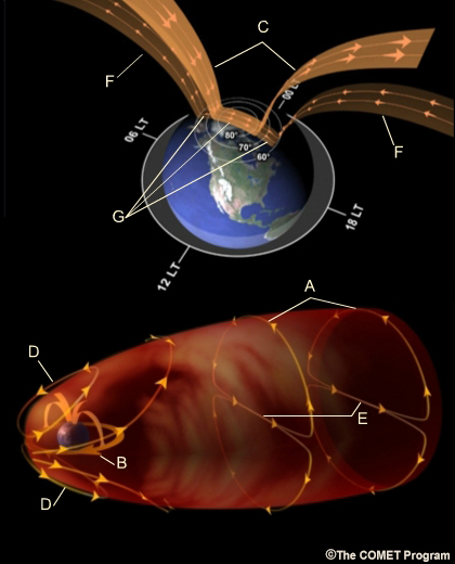
Answer This
Question
Identify the current sytems.
(Use the dropdown
boxes for each description below to choose the corresponding names and
letters on the figures. When finished, click Done.)
Related In-Depth Topics:
Magnetic
Force
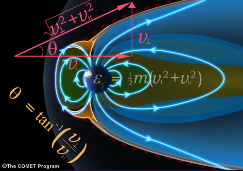
Particle Precipitation Processes
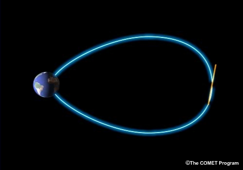
Magnetospheric charged particles on closed magnetic field lines (both ends of which penetrate the earth’s atmosphere) find themselves in a magnetic mirror geometry (learn more about this in the In-depth Topic on Charged Particle Motions). Unless they are traveling nearly parallel to the magnetic field, they bounce back and forth between the Northern and Southern Hemispheres on paths high above the dense regions of the earth’s upper atmosphere.
If, however, their paths are nearly parallel to the field lines, they can reach atmospheric regions where they collide with neutrals. By this process, charged particles precipitate from the magnetosphere into the atmosphere. The range of small pitch angles through which particles are precipitated is called the loss cone.
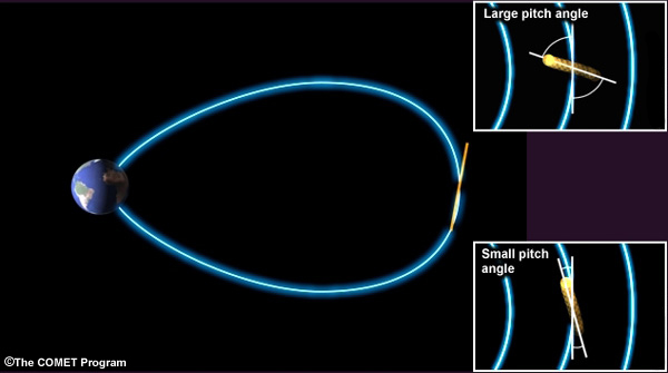
As plasma sheet field lines approach the earth, the loss cone expands. In addition, charged particles can be scattered into the loss cone by magnetic and electrical disturbances in the magnetosphere. Particles precipitated via the loss cone from the magnetosphere into the upper atmosphere produce the aurora.
Related In-Depth Topics:
Charged Particle
Motion
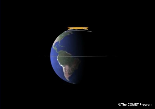
Auroral Oval and its Variations
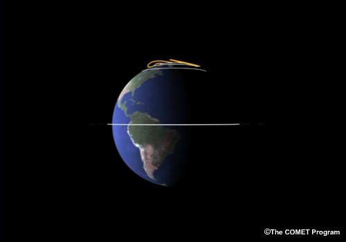
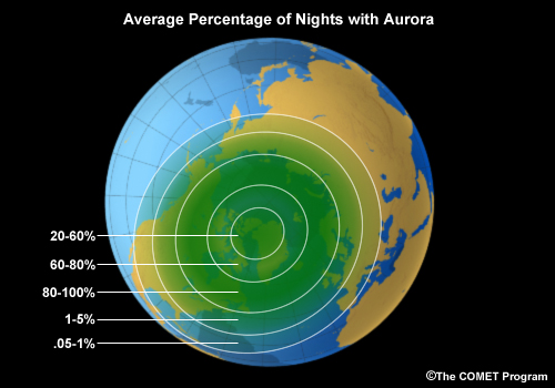
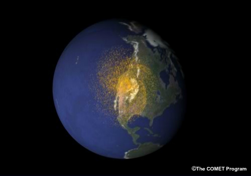
Auroral emissions produced by particle precipitation from the plasma sheet into the atmosphere form elliptical bands of light called auroral ovals, which encircle the magnetic pole in each hemisphere.
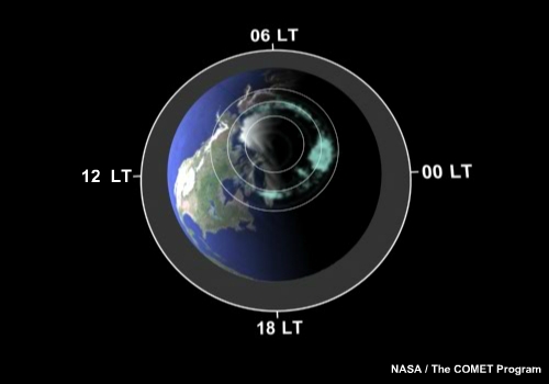
Though ever-present, the ovals brighten and expand during magnetospheric substorms. This brightening and poleward expansion in the midnight sector is caused in the magnetosphere by the formation of a new magnetotail reconnection region some 20 to 30 earth radii down the tail.
During a substorm, very rapid reconnection produces an abundance of energetic plasma sheet particles and a surplus of closed magnetic field in the magnetotail, resulting in increased auroral intensities.
During relatively rare, very strong magnetic storms, this expansion of the auroral ovals is much more extreme, allowing the aurora to be seen as far south (in the northern hemisphere) as Los Angeles, Rome, and Tokyo. After a substorm, the oval returns to its quiet state.
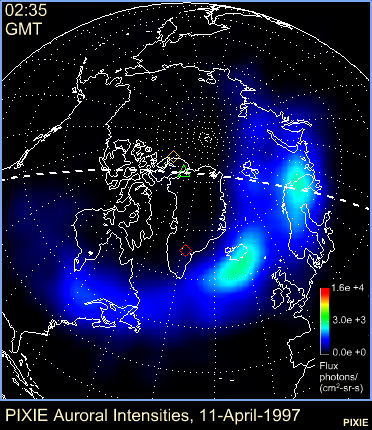
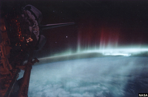
The auroral ovals are best viewed from spacecraft with high inclination orbits; from the ground, only a portion of the auroral oval can be observed from a given location.
Solar Wind and Radiation
In this section, we learned about the solar wind’s tremendous impact on the earth’s magnetosphere. The solar wind shapes and structures the magnetosphere. And it drives key processes such as magnetic reconnection, convection, current systems, and particle precipitation, which produce the aurora and govern the upper atmosphere and ionosphere at high latitudes.
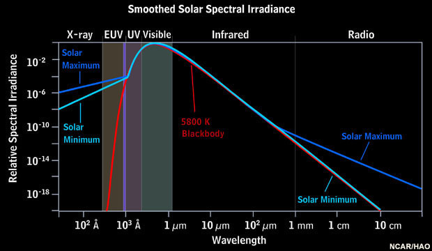
However, we cannot ignore the effects of solar electromagnetic radiation, which carries a million times more energy away from the Sun than the solar wind. Indeed, at lower latitudes the upper atmosphere is controlled almost entirely by solar radiative flux.
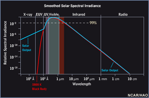
The above graph of solar output, from x-ray to radio wavelengths, shows that some 99% of the radiant energy lies in the visible portion of the spectrum, including near infrared and near ultraviolet (or UV). This visible radiation originates near the solar surface and its intensity does not vary significantly (only about one tenth of 1%) over the 11-year solar activity cycle.
In contrast, extreme ultraviolet (or EUV), and x-ray emissions originate high in the solar atmosphere and vary significantly over the 11-year cycle, and as you will see in the next section, this variation has a major impact on the earth’s upper atmosphere and ionosphere.
Additional Resources:
Upper Atmosphere: Earth's Dynamic Thermosphere-Ionosphere System
Atmospheric Structure
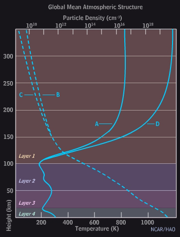
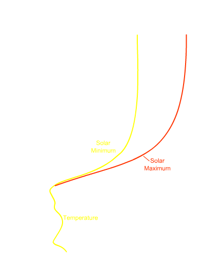
The density of Earth’s atmosphere (shown by the dashed curve on the chart at left below) declines rapidly with height, at a rate determined by the atmospheric temperature (learn more about this in the Static Atmospheres In-depth Topic).
The daytime atmospheric temperature (shown by the solid curve on the chart at left below) at middle and low latitudes strikes a balance between three factors: heating through absorption of solar radiation, cooling through emission of radiation by atmospheric constituents, and transport of thermal energy by atmospheric convection and thermal conduction.
temperature structure
Layers of the atmosphere (shown by the shaded horizontal bands in the chart at left above) are defined in terms of their temperature structure.
Troposphere
In the troposphere, which extends from Earth’s surface to a height of about 15 km, the temperature declines with height, because the surface absorbs most of the solar visible radiation and is heated more efficiently than the overlying atmosphere.
Stratosphere
In the stratosphere, which extends from about 15 km to 50 km, absorption of ultraviolet (UV) radiation by ozone causes temperatures to increase with height.
Mesosphere
The next layer is the mesosphere, between 50 and 100 km altitude. Here, enhanced cooling by CO2 radiation balances heating by far UV radiation so that temperatures decline with height.
Thermosphere
Finally, in the thermosphere, which extends upward from the top of the mesosphere into space, the combined effects of reduced radiative cooling and heating by solar extreme ultraviolet (EUV) radiation cause temperatures to increase up to about 250 km, where a nearly constant value ensues.
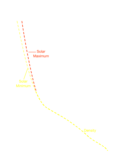
The thermospheric temperature is quite sensitive to variation of the solar EUV radiation over the solar activity cycle. (Click the Solar Cycle Density and Temperature Variability check boxes to see variations over the 11-year solar cycle.)
Explore More
Interactive Irradiance Diagram
Answer This
Question
Identify the layers of the earth's atmosphere, and the
curves representing the global mean atmospheric temperature and
density.
(Use the dropdown boxes for each description below to
choose the corresponding names and layer numbers, and curve letters.
When finished, click Done.)

Related In-Depth Topics:
Static
Atmospheres
The Thermosphere
variability
We have already seen that thermospheric temperature and density are quite sensitive to variation of the solar EUV radiative output over the solar activity cycle. Aside from solar cycle, there are a number of other factors that alter the solar EUV input to the thermosphere, including daily variations produced by the Earth’s rotation, and seasonal variations associated with the Earth’s orbit around the Sun (more about this on the seasonal variability page).
The variation from day to night is quite substantial, though not as large as that produced by solar variability over the solar activity cycle.
See the link to the Interactive Variability Diagram below.
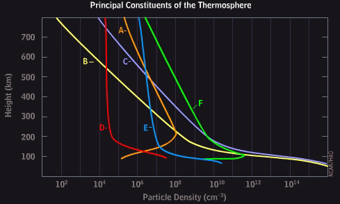
composition
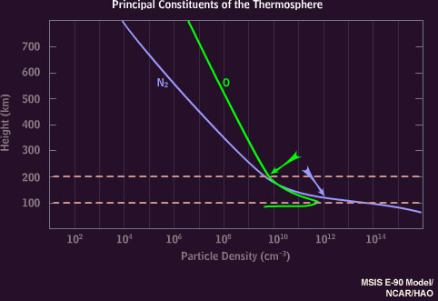
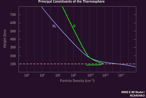
Below the thermosphere, the atmosphere is well mixed in the sense that the density of each atmospheric constituent declines with height at the same rate, unless there is some process that serves to produce or destroy that constituent locally (as in the case of stratospheric ozone). This mixing rapidly diminishes in the thermosphere, where the various atmospheric constituents diffuse through each other, allowing each constituent’s density to vary with height according to its own mass (learn about this diffusion process in the Static Atmospheres). The following chart illustrates this effect.
See the link to the Interactive Variability Composition below.
Notice how the predominance of molecular nitrogen and oxygen at lower levels transitions to atomic nitrogen and oxygen at mid-levels, while at higher altitudes, the lightest thermospheric constituents, He and H, become increasingly predominant.
Explore More
Interactive Variability Diagram
Interactive Composition Diagram
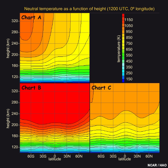
Answer This
Question
How does the thermosphere vary by season and solar
cycle? Find out by analyzing three latitude-height contour plots of
thermospheric temperature. Complete the following statements using the
dropdown boxes.
(When finished, click Done.)
Related In-Depth Topics:
Static
Atmospheres
Thermospheric Dissociation, Mixing, and Diffusion
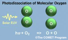
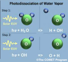
The thermosphere is made up of some constituents, such as molecular nitrogen and oxygen, that are abundant in the air we breathe and others, such as atomic oxygen, nitrogen, helium, and hydrogen, that are relatively scarce near the earth’s surface.
See the link to the Interactive Composition Diagram below.
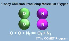
Atomic oxygen, nitrogen, and hydrogen are produced by photo-dissociation, while helium diffuses upward from the earth’s interior. Atomic oxygen, which is the main constituent of the upper thermosphere, is produced by photo-dissociation of molecular oxygen. Nitrogen and hydrogen are the photo-dissociation products of N2 and H2O. (Photo-dissociation of molecular nitrogen; photo-dissociation of water vapor; photo-dissociation of OH.)
The loss of these atoms through recombination is a relatively slow process because a three-body collision is required to conserve both momentum and energy.
Above the turbopause (at about 105 km), the importance of turbulent mixing of atmospheric constituents decreases, allowing the various atoms and molecules to diffuse independently and form density profiles appropriate to their masses. Because gravity is the force pulling the atmosphere downward, the lighter atmospheric constituents feel a weaker downward force, and their density falls off less rapidly.
The following simulation shows the effects of diffusion above the turbopause in an atmosphere with initially uniform composition at all altitudes. Lighter elements that are minor constituents below the turbopause diffuse freely upward to become predominant constituents at higher altitudes.
See the link to the Interactive Interactive Diffusion Simulation below.
Explore More
Interactive Composition Diagram
Interactive Diffusion Simulation
Interactive Chemical Processes Viewer
Answer This
Question
Describe the main constituent of the upper thermosphere
by completeing the following statement.
(Choose an answer from each
of the dropdown boxes. When finished, click Done.)
Related In-Depth Topics:
Static
Atmospheres
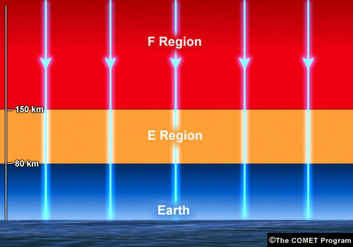
The Ionosphere
ionized plasma
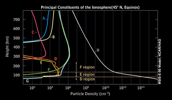
The solar EUV radiation absorbed by the upper atmosphere not only heats the thermosphere (as shown on the previous page), but also ionizes the atmosphere, producing the weakly ionized plasma called the ionosphere. A weakly ionized plasma is an electrically neutral gas (with no net charge) that contains positively and negatively charged particles, as well as a much higher density of neutral particles (shown in the chart below). Such a plasma behaves quite differently from the nearly fully ionized solar wind and magnetospheric plasmas discussed in the Magnetosphere Section and the Charged Particle Motions and Frozen-Field Theorem in-depth topics.
See the link to the Interactive Density Variability Diagram below.
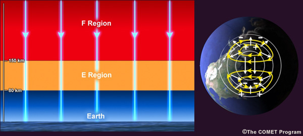
In all but the very lowest part of the ionosphere, the negatively charged particles are electrons, so the ionosphere's structure is generally described in terms of the electron density. The three ionospheric regions (D, E, and F) shown in the above chart are defined by peaks or inflection points in the electron density profile, which produce distinctive signatures in the spectrum of radio waves reflected by the ionosphere.
day-night and solar cycle variations
Like the thermosphere, the ionosphere's density structure is strongly influenced by variations in solar activity and by the day-night variations tied to the earth’s rotation. Click the Solar maximum, Midnight and Solar minimum, Noon checkboxes in the above chart to see these variations.
Corresponding temperature variations (shown in the following graph) are also quite significant. To understand these variations, we must consider the principal physical and chemical processes operating in the ionosphere.
See the link to the Interactive Temperature Variability Diagram below.
Explore More
Interactive Composition Diagram
Interactive Density Variability Diagram
Interactive Temperature Variability Diagram
Related In-Depth Topics:
Static
Atmospheres
Ionospheric Processes
The main processes determining the structure, composition, and variability of the ionosphere are ionization, charge transfer, and recombination. (Follow the links on this page to see animated illustrations of these chemical processes.)
ionization
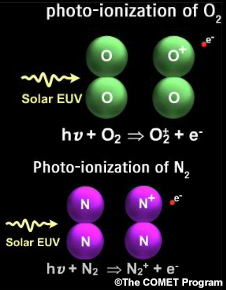
photoionization
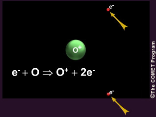
Solar EUV radiation ionizes both molecules and atoms. For example, molecular and atomic oxygen are photoionized to produce molecluar and atomic oxygen ions. (photoionization of molecular oxygen; photoionization of atomic oxygen.)
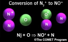
In the case of molecular nitrogen, the photoionization product, molecular nitrogen ions, are rapidly converted into nitric oxide ions.
The EUV photons ionizing the atmosphere generally have much more energy than is required to ionize a molecule or atom, and the excess energy becomes kinetic energy of the electron (called a photoelectron), which provides an important heat source for the thermosphere and ionosphere (more about this on the next page).
collisional ionization
Photoelectrons also ionize the neutral atmosphere, as do galactic cosmic rays and magnetospheric particles (more on this on a related page in the Aurora section).
charge transfer
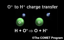
A neutral particle can transfer an electron to an ion. This process is particularly important in the ionization of hydrogen and as a first step in the recombination of atomic oxygen ions.
recombination
dissociative recombination
Dissociative recombination is the most efficient process leading to the loss of molecular oxygen and nitirc oxide ions (O2+ and NO+) in the ionosphere. (recombination of molecular oxygen ions; recombination of nitric oxide ions.)
It is also the final stage in the loss of atomic oxygen ions. (Initial stage: charge transfer between an atomic oxygen ion and molecular nitrogen or molecular oxygen. Final stage: dissociative recombination of the resulting molecular ion—either nitirc oxide or oxygen.)
radiative recombination
Radiative recombination of atomic oxygen ions and other atomic ions is a relatively slow process in the ionosphere (more about this on the next page).
Structure and Variability of the Ionosphere
ionized plasma
The low and midlatitude ionosphere is produced by photoionization of the neutral atmosphere, so its composition reflects that of the neutral atmosphere.
In the E region, photoionization of N2 and O2 yields NO+ and O2+ as the main constituents, while in the F region, photoionization of O makes O+ the principal constituent (these processes are illustrated on the preceding page). At high altitudes, the midlatitude ionosphere is called the plasmasphere (more about the plasmasphere on the magnetospheric convection page) and is dominated by its lightest constituent, H+.
See the link to the Interactive Composition Diagram below.
day-night density variations
At night, photoionization ceases, and dissociative recombination (described on the preceding page) steadily lowers the ionosphere's density. (Click the Solar maximum, Midnight checkbox on the chart below to compare day and nighttime densities.)
See the link to the Interactive Density Variability Diagram below.
This effect is most pronounced in the E region, where the neutral molecular density is highest. In the F region, where dissociative recombination slows, radiative recombination is not fast enough to significantly deplete the electron density. Downward flow of plasma from the plasmasphere also helps to maintain F-region density at night.
day-night temperature variations
Photoelectrons, which are instrumental in heating the thermosphere and ionosphere, transfer their energy most efficiently to the lightest particles, the ambient electrons. The next most efficient energy transfer is to the ions (because of their electric charge). So during the day, the electron temperature is much higher than the ion and neutral temperatures (as shown in the chart below). At night, when no new photoelectrons are produced, the electrons and ions cool through collisions with neutrals, and the neutrals cool by radiation (called airglow).
See the link to the Interactive Temperature Variability Diagram below.
Explore More
Interactive Composition Diagram
Interactive Density Variability Diagram
Interactive Temperature Variability Diagram
Answer This
Question
Describe the processes governing the ionophere by
completeing the following statement.
(Choose an answer from each of
the dropdown boxes. When finished, click Done.)
Related In-Depth Topics:
Static
Atmospheres
Seasonal Variability of the Ionosphere
The Earth’s annual journey around the Sun causes seasonal changes in the thermosphere and ionosphere.
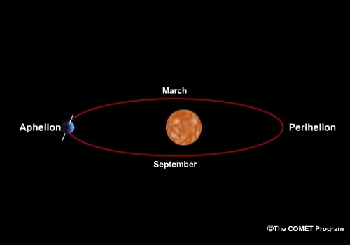
During summer, solar radiation warms the thermosphere and ionosphere (shown in the chart below), just as it does during both daytime and solar maximum.
See the link to the Interactive Seasonal Density Variability Diagram below.
But, as shown in the following graph, higher summer temperatures do not increase densities in either the upper thermosphere or the F region of the ionosphere.
See the link to the Interactive Seasonal Temperature Variability Diagram below.
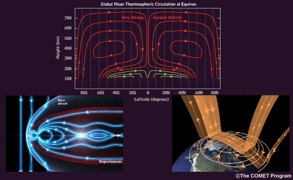
Why would densities increase with noonday and solar max heating, while decreasing with summer heating? To make sense of this paradox, we need to consider large-scale circulations in the thermosphere.
At equinox, thermospheric heating is strongest near the equator (see the graph below). This creates a convection pattern with fountain-like upwelling at low latitudes and sinking at high latitudes.
See the link to the Interactive Thermospheric Circulation Diagram below.
At solstice (click the Northern and Southern Summer Solstice buttons on the graph above), the circulation pattern shifts significantly, with upwelling in the summer hemisphere and the sinking in the winter hemisphere.
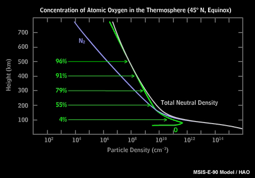
The concentration of atomic oxygen (shown in the above graph) increases from 4% at the base of the thermosphere to 96% by 500 km. This means that upwelling in the thermosphere carries oxygen-poor air upward in the summer hemisphere while oxygen-rich air sinks downward at the other end of the circulation. Summer heating has the net effect of depleting the summer hemisphere of atomic oxygen. Photoionization in the oxygen-rich winter thermosphere makes the F-region ionosphere denser as well. (To see these effects, compare summer and winter curves on the below chart of electron and neutral particle densitites in the ionosphere, which show that atomic oxygen and electron densities are higher in the winter hemisphere F region.)
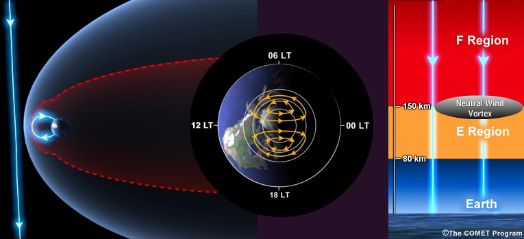
Electrodynamic Coupling
An electric generator, or dynamo, operates by turning a coil in the presence of a magnetic field, thus converting mechanical energy into electrical energy.
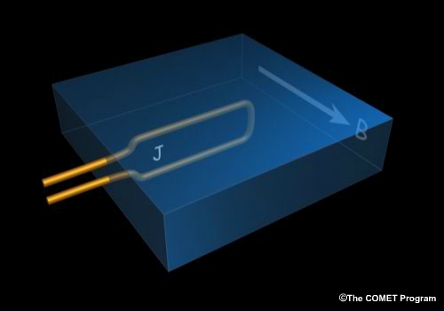
The same type of mechanical-electrical coupling is involved when a thermospheric wind blowing across the magnetic field generates electric fields and currents. A good example of this electrodynamic coupling is the atmospheric dynamo.
In the E region of the ionosphere, winds generate an electric field perpendicular to the magnetic field, producing two electric currents. One, carried by ions in direction of the electric field, is a Pedersen current. The other, carried by electrons in the direction of -E x B, is a Hall current. (Learn more about particle drifts in the Charged Particle Motions in-depth topic.)
To understand how this atmospheric dynamo works, imagine you are 100 km above the Northern Hemisphere in the E region of the ionosphere.
The magnetic field is directed downward into the earth and a counterclockwise horizontal neutral wind vortex is blowing. At this level, ions collide constantly with neutrals and are carried along in the vortex flow. The magnetic force perpendicular to the flow and field causes the ions to drift towards the center of the vortex. As they accumulate in the center, a positive charge builds there, while a negative charge builds in the region vacated by the ions, resulting in an outward-directed polarization electric field.
The effects of this electric field are felt both above and below the vortex. In the lower E region, the field induces a clockwise Hall current vortex through E x B drift of electrons. In the F region, above the vortex, the air is less dense and ions have fewer collisions, so this electric field stirs a counterclockwise plasma vortex through the E x B drift of both ions and electrons.
Related In-Depth Topics:
Charged Particle
Motions
Magnetic
Force
Frozen-Field
Theorem
Interconnections
The ionosphere interconnects with the magnetosphere along magnetic field lines. At low and middle latitudes, the magnetospheric extension of the ionosphere is called the plasmasphere, a region of cool, highly ionized plasma (T ~ 3000 K ~ 0.3 eV).
At higher latitudes, where magnetospheric particles precipitate downward into the auroral oval, ionospheric plasma also extends upward into the magnetospheric plasma sheet to mix with energetic particles (>10 keV) from the magnetotail.
At the highest latitudes, the polar cap ionosphere expands supersonically into the dayside cusp, plasma mantle, and magnetotail lobes, where it mixes with hot, tenuous plasma originating in the solar wind.
At low and middle latitudes, EUV solar radiation shapes and controls the thermosphere-ionosphere. At the higher latitudes of the auroral ovals, energetic particles from the plasma sheet exert the greatest influences on the thermosphere-ionosphere.
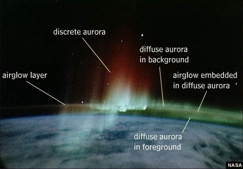
Although nearly half of the EUV radiation absorbed in the thermosphere is eventually re-radiated as UV airglow, the airglow is not discernable from the ground during daytime (because of the bright sky background), and the residual airglow at night is relatively weak and diffuse. In contrast, auroral displays are much brighter, more structured, and dynamic because they are generated by energetic particles from the highly dynamic magnetospheric plasma sheet.
Our next section explains how these energetic particles work their magic.
Aurora: How Particle Processes and Current Systems Generate Aurora
Introduction
Auroral displays are the most dramatic example of physical processes taking place in near-earth space.
They can change from faint, still bands to great bursts of rapidly moving color in a matter of seconds, often appearing to almost touch the ground, other times towering in the sky to tremendous height.
In fact, auroral light comes from altitudes of about 100 to 200 kilometers, a region that is both the farthest reaches of the upper atmosphere and the nearest part of space.
The aurora is usually confined to oval-shaped regions around the magnetic poles of the earth. These ovals are also displaced toward the night side of the earth.
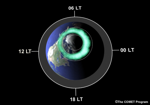
When auroral activity is quiet, the ovals are about 3000 kilometers across, but when it intensifies, the ovals grow in diameter to 4000 or 5000 kilometers. Because the north magnetic pole is in northern Canada, the aurora borealis is most often seen at populated latitudes in the western hemisphere. The aurora australis can be visible during from the island of Tasmania or southern New Zealand.
Particle Sources
Auroral displays are caused by energetic particles flowing along magnetic field lines from deep in the magnetotail to the upper atmosphere. Most of these particles are electrons, but protons and other ions may also be present.
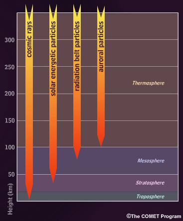
Auroral particles are one of the many categories of energetic particles that bombard the Earth. These include extremely high-energy fluxes of particles in the GeV or MeV range, such as cosmic rays, high-energy radiation belt particles, and solar energetic particles. Auroral particles originating in the magnetospheric plasma sheet are generally in the 1 to10 keV energy range, but can sometimes be as high as 100 keV. Less energetic particles (in the 100s of electron-volts) such as solar wind entering the magnetosphere in the dayside cusp regions near the magnetic poles, also impact the upper atmosphere.
| Cosmic Rays | Solar Energetic Particles | Radiation Belt Particles | Auroral Particles | Solar Wind Particles | |
|---|---|---|---|---|---|
| Types |
protons
|
mostly protons
|
electrons and protons
|
electrons and protons
|
electrons and protons
|
| Sources |
interstellar space
|
the Sun
|
|||
| Energy Ranges (eV) |
109 - 1018+
|
107 - 109
|
106 - 107
|
103 - 105
|
102
|
The depth to which particles penetrate the atmosphere depends on their energy; the more energetic they are, the deeper they travel. Cosmic rays can reach the troposphere or even the surface of the Earth; solar energetic particles and radiation belt particles can reach the stratosphere and mesosphere; and auroral particles reach the lower thermosphere, usually around 100 kilometers. Auroral particles entering the atmosphere are far more numerous than the others, which is why auroral displays are seen.
Collisions and Emissions
As charged particles precipitate from the magnetosphere into the upper atmosphere, they collide with the tenuous gases there.
Each collision imparts some of the particle's energy to the atom or molecule it hits. The incoming particles also ionize, dissociate, or excite the atoms or molecules they collide with. When ionization occurs, the ejected electrons, called secondary electrons, also carry excess energy. They, in turn, cause additional ionization, dissociation, and excitation.
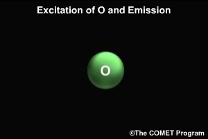
Excitation results in emission. Excited states are unstable, and atoms emit light of specific wavelengths as they decay back down to a stable configuration. This process can be compared to a cathode ray tube such as a television screen or computer monitor, where electron beams hit a phosphor surface, changing the energy level of the phosphor molecules and causing them to emit light.
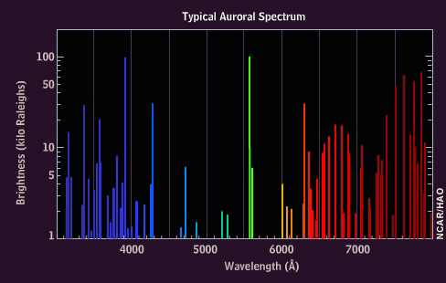
Unlike sunlight, auroral light is not a continuous spectrum of wavelengths. Rather, it is made up of discrete colors at specific wavelengths, because it is caused by emissions from excited states of atmospheric gases.
Auroral emissions also result from chemical reactions that occur among the ionized and dissociated gases.
Auroral Colors and Spectra
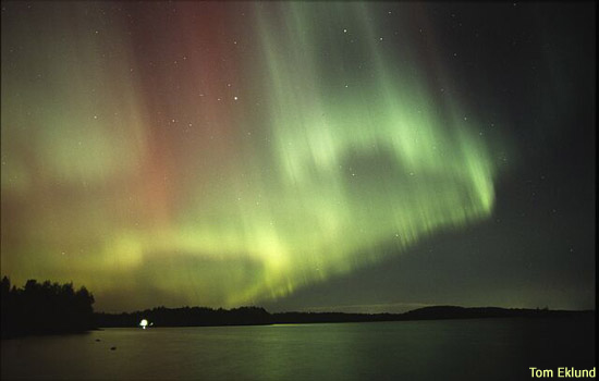
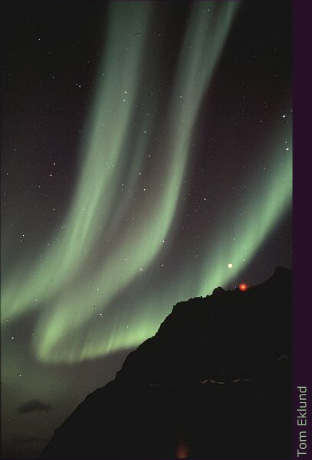
When the aurora is faint, it appears white to the unaided eye. As its brightness increases, color vision starts to work, and the characteristic pale green hue of the aurora becomes visible.
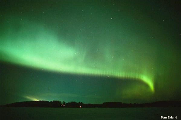
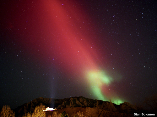
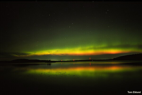
With more intensity, a bright green color is visible in the lower regions, and a faint red glow can be discerned at high altitude.

When the aurora is very energetic and very bright, a deep red lower border appears below the green.
The atmosphere above 100 kilometers consists mainly of nitrogen molecules and oxygen atoms, with more nitrogen at 100 kilometers transitioning to proportionally more oxygen at 200 kilometers.
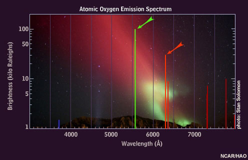
When oxygen atoms are excited, they emit light of various colors, but the brightest are the red and green emissions.
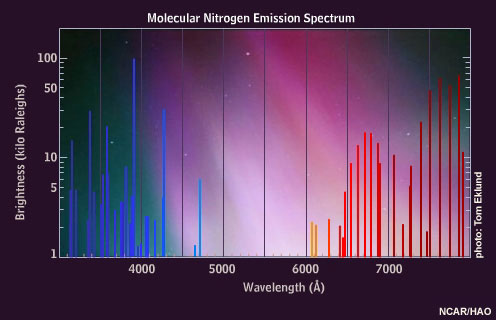
Excited nitrogen molecules emit red, blue, and violet light. The interplay of oxygen and nitrogen and their proportional changes with altitude cause the typical appearance of auroral colors.
Some of the excited nitrogen molecules also interact with the atomic oxygen, causing an additional green emission at a wavelength of 558 nanometers. This emission, called the "auroral green line," is seen throughout the aurora down to about 100 kilometers, giving the aurora its dominant green appearance.
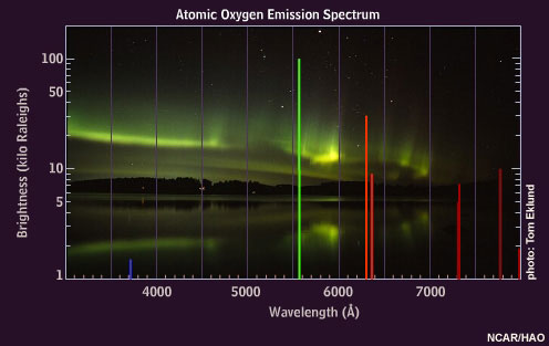
Oxygen atoms emit 630 nanometer "auroral red line" light only at very high altitudes because these atoms are de-excited by collisions with nitrogen molecules below about 150 kilometers.
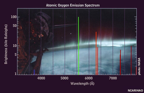
The auroral green line disappears below 100 kilometers, where little atomic oxygen exists.
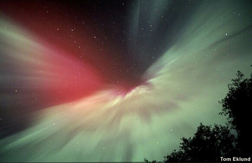
When highly energetic particles reach low levels, they trigger the red, blue, and violet emissions of molecular nitrogen, observed as a deep red or magenta border at the lower edge of auroral curtains. This dramatic effect is enhanced by the rapid motion associated with these very energetic displays. It is also possible to see waves of green light "chasing" the magenta, an effect caused by the time lag between excited oxygen and nitrogen. Oxygen atoms persist for about one second in their unstable state before decay, while the nitrogen molecule emissions are instantaneous.

High-Latitude Ionosphere
The magnetosphere not only supplies energetic particles that cause the aurora, but it also drives strong winds and electric currents in the high-latitude ionosphere and thermosphere.
The magnetospheric convection that carries plasma and magnetic field from the dayside magnetopause into the magnetotail and back again also stirs winds in the high latitude ionosphere and thermosphere. These winds circulate from the dayside auroral ovals across the polar caps to the night side, then around the dawn and dusk sides back to the dayside.
In the lower part of the ionosphere, from about 80 to 150 kilometers, the electric field associated with the magnetosphere-ionosphere circulation drives strong horizontal electric currents.
Because of the peculiar nature of ionospheric conductivity, there are actually two high-latitude current systems. One system comprises Hall currents, which flow perpendicular to both the electric and magnetic fields and are strongest near 105 kilometers altitude. The other system is made up of Pedersen currents, which flow perpendicular to the magnetic field and parallel to the electric field and are strongest near 125 kilometers altitude. These two ionospheric current systems connect via field-aligned currents to the magnetospheric current system.
The Atmospheric Dynamo
Magnetospheric convection drives winds and currents in the high-latitude ionosphere, but this is a coupled system; the ionosphere also exerts dynamical influences on the magnetosphere. Two examples of this influence are the high-latitude atmospheric dynamo and ionospheric conductivity anomalies.
In a motor, the flywheel’s inertia moderates speed fluctuations in other parts of the machinery. A similar effect occurs with the atmospheric dynamo, which is introduced in the Upper Atmosphere section of this module.

Consider, for example, the case of a southward solar wind magnetic field. The twin flow vortices of the high-latitude ionospheric plasma circulation frictionally accelerate the neutral atmosphere to produce similar, neutral wind vortices in the upper E region and lower F region.
If the solar wind magnetic field shifts, removing the electric field driving these circulations, the neutral wind vortices will continue spinning for some time, driving (through dynamo action) ionospheric and magnetospheric motions similar to, but weaker than, the original motions. The neutral wind here behaves just like a mechanical flywheel.
Auroral Storms
Auroral storms have tremendous impacts on the thermosphere and ionosphere. As the auroral oval intensifies and expands, more energy flows through the system, and there is more ionization and heating.
Much of the heating comes from collisions between ions set in motion by auroral currents and the neutral atmosphere. This frictional heating, or Joule heating, causes upwelling of the atmosphere in the auroral zone, and during times of intense geomagnetic disturbances, can even reverse the global circulation pattern.
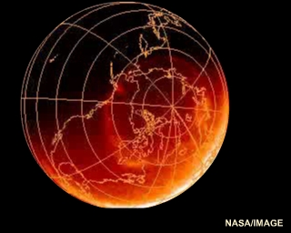
(The dramatic auroral storm movie above was recorded by the Far Ultraviolet (FUV) Imaging System on the IMAGE spacecraft. The storm occurred 15-16 July 2000. For more information, visit the IMAGE: FUV/WIC Website.)
When there are no auroral storms heating the thermosphere, solar heating drives the convection. At equinox, for example, strong heating near the equator causes air to rise at low latitudes and sink at high latitudes, in a fountain-like circulation pattern.
Weak auroral heating reverses this circulation at high altitudes and latitudes.
As the heating increases, the reversal expands.
During geomagnetic storms, auroral heating can be strong enough to reverse the circulation throughout most of the thermosphere.
Wave-like disturbances also travel through the ionosphere in response to these auroral storms and sub-storms, causing disruptions of communication and navigation systems. The response of the ionosphere to geomagnetic disturbances is thus extremely complex, challenging to model, and difficult to predict.
Additional Resources:
IMAGE:
FUV/WIC Website
Expole More
Associations
The next time you happen across the mysterious and beautiful dancing lights of the aurora, you might think of the magnetosphere, source of energetic particles that create the auroral light and generator of electric currents that heat the polar ionosphere.
Or your mind may turn to the Sun and solar wind, whence nearly all magnetospheric particles and energy derive.
Or perhaps you will see in your mind’s eye a giant fountain of air rising from the polar atmosphere and settling in the tropics, high above the ground.
You might even wonder whether this auroral storm has disrupted communications and navigation systems, or endangered astronauts in space.
But wherever your mind may wander, borne by this dazzling display, may you never lose the
same sense of mystery that our ancestors felt when beholding this amazing and beautiful
silent fire in the polar sky.
Review: Module Summary
Mystery
From the dawn of humankind, the aurora has invoked a deep sense of mystery in all who have viewed it. Although there has been an abundance of explanations of this strange phenomenon, ranging from the mythical to the scientific, it is only over the last century that an understanding with a sound physical basis has developed.
This module provides a description of our current understanding of the aurora, focusing on the most important physical and chemical processes underlying its origin.
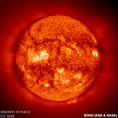
Magnetosphere
The story of the aurora begins at the Sun, where the solar corona (the hot, outermost atmosphere of the Sun) expands outward in a hypersonic flow called the solar wind. As the solar wind passes the Earth, it interacts strongly with the nearly dipolar terrestrial magnetic field, compressing it on the dayside and dragging it into a comet-like tail on the nightside, forming the earth's magnetosphere.
The solar wind carries with it a magnetic field, and as the wind interacts with the magnetosphere, the solar wind magnetic field interconnects with the terrestrial magnetic field, allowing the direct entry of solar wind plasma into the magnetosphere and producing a tangential stress along the magnetopause, the outer boundary of the magnetosphere. This tangential stress drives large-scale convection in the magnetosphere and in the ionosphere, the ionized part of the earth's upper atmosphere.
Entry of hot solar wind plasma into the magnetosphere, along with the outward flow of cool plasma from the ionosphere, leads to a mixed plasma in the central portion of the magnetotail, which is called the plasma sheet. Convective plasma flow from the tail of the magnetosphere toward the Earth compresses and heats the particles in the plasma sheet, populating the near-earth magnetosphere with energetic particles. It is these particles that are able to make their way down magnetic field lines into the earth's high-latitude upper atmosphere, where they excite atoms and molecules to produce the dancing lights of the aurora.
Interaction of the solar wind with the magnetosphere leads not only to plasma convection and particle precipitation into the upper atmosphere, but also to a complex set of electrical currents. These currents flow along the magnetopause, through the center of the magnetotail, and around the earth in the inner magnetosphere. The magnetospheric currents also flow along magnetic field lines and through the high-latitude ionosphere, where they deposit energy comparable to that deposited by precipitation of plasma sheet particles into the auroral zone.
Upper Atmosphere
Solar EUV radiation varies significantly over the 11-year solar activity cycle, and the EUV input to the upper atmosphere also varies with the day-night cycle, as well as with the seasons.
This radiation is responsible for dissociating molecular atmospheric constituents, ionizing atoms and molecules, and heating the atmosphere. As a result, the upper atmospheric temperature, density, composition, and ionization state all vary as the intensity of the incoming solar EUV radiation varies.
The ions and electrons produced by solar EUV radiation form what is called the ionosphere, which is just the ionized part of the upper atmosphere.
Click here to view the Interactive Composition Diagram.
At middle and low latitudes, cool ionospheric plasma extends along magnetic field lines into the magnetosphere to form the plasmasphere, which is the only part of the magnetosphere not taking part in the large-scale convection process.

At high latitudes, cool ionospheric plasma flows into the magnetosphere, where it mixes with hot solar wind plasma and may provide a significant number of the particles in the plasma sheet. These particles are then energized and eventually precipitated into the atmosphere to produce the aurora.

Aurora
Auroral displays are caused by energetic particles flowing along magnetic field lines from deep in the magnetotail to the upper atmosphere. Auroral particles penetrate the lower thermosphere, usually around 100 km altitude. The incoming particles excite atoms and molecules they collide with, producing emissions at specific wavelengths.
Interactive Auroral Spectra Viewer
Heating in the auroral zones, which is associated with the dissipation of ionospheric currents and the precipitation of magnetospheric particles, can have a major impact on the global upper atmospheric circulation pattern.
Interactive Thermospheric Circulation Diagram
During periods of weak auroral activity, this circulation (near equinox) is characterized by a rising of air near the equator (site of maximum radiative heating) and a sinking at high latitudes. During strong auroral storms, this circulation pattern can be nearly reversed, because of the very strong auroral heating at high latitudes.
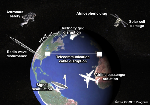
Strong auroral storms can also affect a number of the high-technology systems on which our present-day society is so dependent, such as communication and navigation systems, power grids, satellite attitude control, and satellite orbits.

The aurora will always offer us inherent beauty and mystery. But it also provides significant challenges, including the need to understand the physics of a complex and intriguing physical system extending from the Sun to the Earth and the impacts this system has on our technological society.

Resources
Educational Materials and Aurora Imagery
- American Geophysical Union
- Electricity and Magnetism Video Lectures by MIT's Walter Lewin
- Eric Weisstein's World of Physics
- Exploratorium Web Page on the Aurora
- From Stargazers to Starships
- High Altitude Observatory Education Pages
- Johns Hopkins University Auroral Particles & Imagery Group
- NASA Mission to Geospace
- Space Environment Center Educational Materials
- Tom Eklund Aurora Photos and Links
- Visual Tour of Classical Electromagnetism
- Windows to the Universe
Space Weather Data
- CANOPUS Real Time Auroral Oval
- Fast Auroral Snapshot Explorer
- Imager for Magnetopause-to-Aurora Global Exploration
- LASCO/SOHO Coronagraph, Naval Research Laboratory
- NOAA Space Weather Prediction Center
- Poker Flat Research Range, Fairbanks, Alaska
- Solar and Heliospheric Observatory (SOHO)
- Spaceweather.com
Data & Imagery Sources
The following sources provided data and imagery for Physics of the Aurora: Earth Systems.
- International Reference Ionosphere - IRI-2001 provided by National Space Science Data Center (NSSDC). [Available online at https://iri.gsfc.nasa.gov/iri.html]
- MSIS-E-90 Atmosphere Model, developed by A.E., Hedin, is provided by NSSDC. [Available online at https://ccmc.gsfc.nasa.gov/modelweb/models/msis_vitmo.php]
- Grassman, Ampere, Newton Photographs http://www-groups.dcs.st-and.ac.uk
References
- Aristotle, Meteorologica, trans. E.W. Webster
- Carlowicz, M. and Lopez, R. (2002), Storms from the Sun. Washington DC: Joseph Henry Press, pp. 64-66.
- Einstein, A., The World as I See It, translated by A. Harris, Watts and Company, London, 1940.
- Friedman, H. (1986), Sun and Earth. New York: Scientific American Books, pp. 165-166.
- Galileo, G., Le Opere di Gilileo Galilei, 2nd ed., Edizione Nazionale, Florence, 1929-1939; cited in Majestic Lights: The Aurora in Science, History and the Arts, p. 48.
- Griffiths, David J., Introduction to Electrodynamics, Prentice-Hall, New Jersey, 1999.
- Halley, E., An account of the late surprising appearance of the lights seen in the air, Phil. Trans. Roy. Soc., 29, 406, 1716; cited in Majestic Lights: The Aurora in Science, History and the Arts, pp 50-52.
- Leach, M. (Ed.), Standard Dictionary of Folklore, Mythology and Legend, Funk and Wagnals, New York, 1949.; cited in Majestic Lights: The Aurora in Science, History and the Arts, p. 114.
- Lewin, W., Electricity and Magnetism, Spring 2002. Massachusetts Institute of Technology. [Available online at https://ocw.aprende.org/courses/physics/8-02-electricity-and-magnetism-spring-2002/ ]
- Longfellow, H.W., The Song of Hiawatha, Tickner and Fields, Boston, 1885.
- Maccabees II (5:2)
- Nansen, F., Eskimo Life, Longmans, Green and Company, London. 1893; cited in Eather, R. H. Majestic Lights: The Aurora in Science, History and the Arts. Washington D.C.: American Geophysical Union, 1980, p. 110.
- Seneca, Naturales Quaestiones, Book 1, translated by T.H. Corcoran, Harvard University Press, Cambridge, MA., 1972; cited in Majestic Lights: The Aurora in Science, History and the Arts, p. 39.
Contributors
Funding Provided By
- National Science Foundation (NSF)
- National Weather Service (NWS)
Principal Science Advisor
- Tom Holzer — NCAR/HAO
Contributing Science Advisors
- Arturo Lopez Ariste — NCAR/HAO
- Alan Burns — NCAR/HAO
- Sarah Gibson — NCAR/HAO
- Maura Hagan — NCAR/HAO
- Gang Lu — NCAR/HAO
- Astrid Maute — NCAR/HAO
- Stan Solomon — NCAR/HAO
- Wenbin Wang — NCAR/HAO
- Michael Wiltberger — NCAR/HAO
Project Co-Lead/Science Content Development & Coordination
- Dolores Kiessling — UCAR/COMET
Project Co-Lead/Intructional Design/Multimedia Development
- Dwight Owens— UCAR/COMET
Programming Support
- Dan Riter — UCAR/COMET
Audio Editing/Production
- Seth Lamos — UCAR/COMET
Computer Graphics/Interface Design
- Heidi Godsil — UCAR/COMET
Illustration/Animation
- Steve Deyo — UCAR/COMET
Software Testing/Quality Assurance
- Michael Smith — UCAR/COMET
- Linda Korsgaard — UCAR/COMET
Copyright Administration
- Lorrie Fyffe — UCAR/COMET
Audio Narration
- Chet Sisk
Aurora Photography
- Tom Eklund
- Stan Solomon — NCAR/HAO
Aurora Videography
- Greg Syverson — Alaska Bristol Bay Photography
Data Provided by
- NASA
- National Space Science Data Center (NSSDC)
COMET HTML Integration Team 2021
- Tim Alberta — Project Manager
- Dolores Kiessling — Project Lead
- Steve Deyo — Graphic Artist
- Ariana Kiessling — Web Developer
- Gary Pacheco — Lead Web Developer
- David Russi — Translations
- Tyler Winstead — Web Developer
COMET Staff
Director
- Dr. Timothy Spangler
Deputy Director
- Dr. Joe Lamos
Meteorologist Resources Group Head
- Dr. Greg Byrd
Business Manager/Supervisor of Administration
- Elizabeth Lessard
Administration
- Lorrie Fyffe
- Heather Hollingsworth
- Linda Korsgaard
- Bonnie Slagel
Graphics/Media Production
- Steve Deyo
- Heidi Godsil
- Seth Lamos
- Dan Riter
Hardware/Software Support and Programming
- Tim Alberta (Supervisor)
- James Hamm
- Karl Hanzel
- Andrew Jurey (Student)
- Ken Kim
- Mark Mulholland
- Carl Whitehurst
Instructional Design
- Patrick Parrish (Supervisor)
- Dr. Alan Bol
- Lon Goldstein
- Dr. Vickie Johnson
- Bruce Muller
- Katherine Olson
- Dr. Sherwood Wang
Meteorologists
- Dr. William Bua
- Patrick Dills
- Tom Dulong
- Kevin Fuell
- Patrick Hofmann (Student)
- Dr. Stephen Jascourt
- Matthew Kelsch
- Dolores Kiessling
- Dr. Richard Koehler
- Dr. Arlene Laing
- Heather McIntyre (Student)
- Wendy Schreiber-Abshire
- Dr. Doug Wesley
Software Testing/Quality Assurance
- Michael Smith (Coordinator)
National Weather Service COMET Branch
- Anthony Mostek (NWS COMET Branch Chief [acting] and Satellite Training Leader)
- Brian Motta
- Dr. Robert Rozumalski (SOO Science and Training Resource [SOO/STRC] Coordinator)
- Shannon White (IFPS Training)
Meteorological Service of Canada Visiting Meteorologists
- Peter Lewis
- Garry Toth