In-Depth Topics
Table of Contents
How do ions and electrons move under the influences of magnetic, electric, and gravitational fields? What happens when they collide? Have you ever had a magnetic moment, when your mirror geometry kept you coming back again and again?
Does the subject of magnetic pressure make you tense? Maybe you need more force balance in your life! With some help from André Ampère, you can learn how to balance your plasma momentum and find the equilibrium current you've been looking for.
Do you ever get the feeling that even though your life is in flux, your identity remains frozen, unable to escape the bounds of society's ambient plasma? Despair not, for it is possible to break the field! Rapid spatial changes can make all the difference.
You may be familiar with the discomfort of dense gas pressure, but what about the frigid heat of a tenuous gas? How can something so hot feel so cold?
Charged Particle Motion
-
A particle with charge
 moving with velocity
  in a uniform magnetic field
  experiences a
force:
experiences a
force:
The force on the particle is perpendicular to both the velocity and magnetic field and thus does no work on the particle.
If the velocity is perpendicular to the magnetic field, the particle moves in a circle of radius
 with centripetal acceleration
  . Equating the magnetic force to the particle mass
  times the
centripetal acceleration, we can show that the radius of gyration (or gyroradius) of
the particle is equal to
times the
centripetal acceleration, we can show that the radius of gyration (or gyroradius) of
the particle is equal to  . (Watch the video below to see the
formulation):
. (Watch the video below to see the
formulation): For a given gyroradius, the corresponding frequency of gyration (or gyrofrequency), expressed in radians per second, is
 . (Watch the video below to see the
expression):
. (Watch the video below to see the
expression):If a component of the particle's velocity (
 ) is parallel to the magnetic field, then
  is
replaced by
is
replaced by  in the preceding two equations, while the component carries the particle along the magnetic field, creating a
helical trajectory.
in the preceding two equations, while the component carries the particle along the magnetic field, creating a
helical trajectory.
Motion in a Uniform Magnetic Field
-
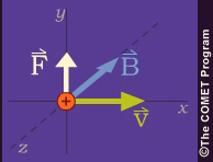
If a uniform electric field,
 , is added the magnetic field , the charged
particle experiences a force:
, is added the magnetic field , the charged
particle experiences a force:
in addition to the magnetic force:

The total force on the particle is thus:

Only the electric force can do work on the particle since the magnetic force is always perpendicular to the particle velocity. If both
and are
perpendicular to ,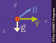
acceleration by the electric field changes the circular motion shown on the Motion in a Uniform Magnetic Field section.
In the segment of its orbit when the particle is moving in the direction of the electric force, it accelerates, and its gyroradius expands. When it moving against the electric force, it decelerates and its gyroradius contracts. These distortions of the gyroradius cause the particle to drift in a direction perpendicular to both
and . Notice in the following animation how the velocity increases during the particle's downward swing, reaching its maximum at the base of the orbit. The veclocity vector has a rightward component during the half of the orbit when it is strongest, while it has a leftward component during the half when velocities are weakest. The net effect is a rightward drift.
These distortions of the gyroradius cause the particle to drift in a direction perpendicular to both
and . The average drift velocity is given by: 
This kind of drift can be induced by any effect that modifies a particle’s gyroradius over the course of its orbit.
Particle Drifts
-
Question 1
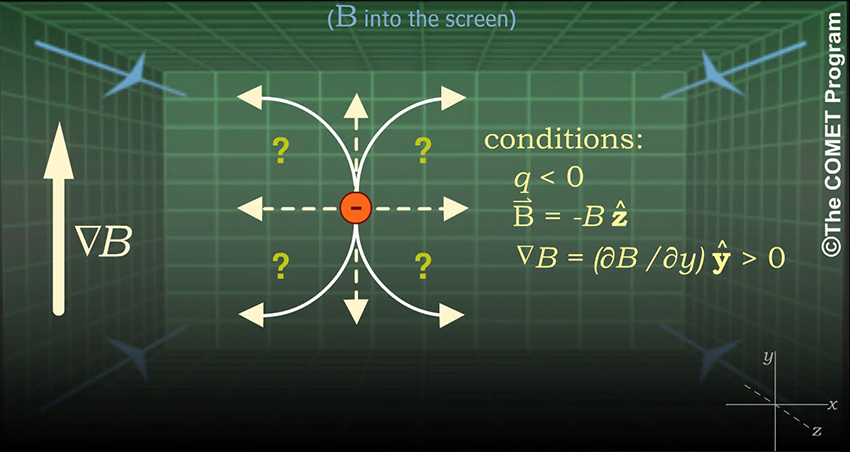
In the illustration in the Particle Drift section, we looked at a positively charged particle. What if we substitute a negatively charged particle (e.g., an electron)? What will be its directions of orbit and drift?
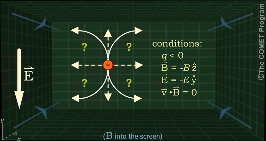
Given these conditions, how will the electron behave?
(Choose answers to complete the sentence, then click Done.)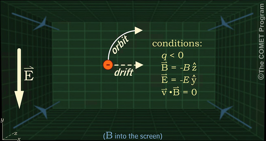
The electron orbits clockwise, in the direction opposite to that of the positively charged particle, because the magnetic force on a charged particle depends on the sign of the charge.
The electron drifts toward the right because its maximum gyroradius is at the top of its clockwise orbit. A positively charged particle would also drift toward the right because its maximum gyroradius is at the bottom of its counterclockwise orbit.
Question 2
How about an electron under the influence of an nonuniform magnetic field? In this question, the magnetic field goes from strong at the top to weak at the bottom. How will such a field influence particle motions?
Given these conditions, how will the electron behave?
(Choose answers to complete the sentence, then click Done.)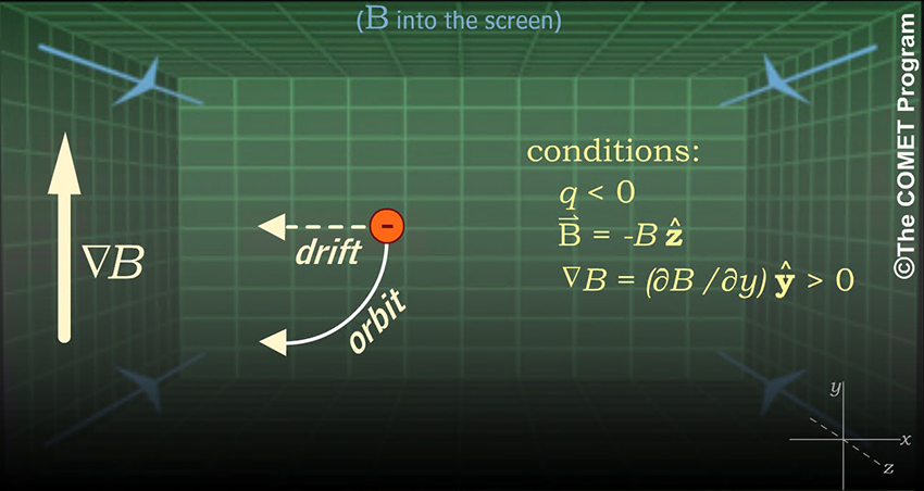
The electron orbits clockwise, in the direction opposite of a positively charged particle, because the magnetic force on a charged particle depends on the sign of the charge.
The electron drifts toward the left because its orbit is clockwise and its maximum gyroradius is at the bottom of its orbit (as a result of the weaker magnetic field there). A positively charged particle would drift toward the right because its orbit is counterclockwise, but its maximum gyroradius is also at the bottom of its orbit.
Question 3
How about a proton under the influence of a uniform gravitational field? In this question, the gravity is directed downward. How will gravitational acceleration influence the proton's motions?
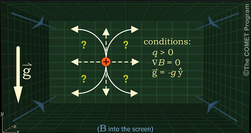
Given these conditions, how will the proton behave?
(Choose answers to complete the sentence, then click Done.)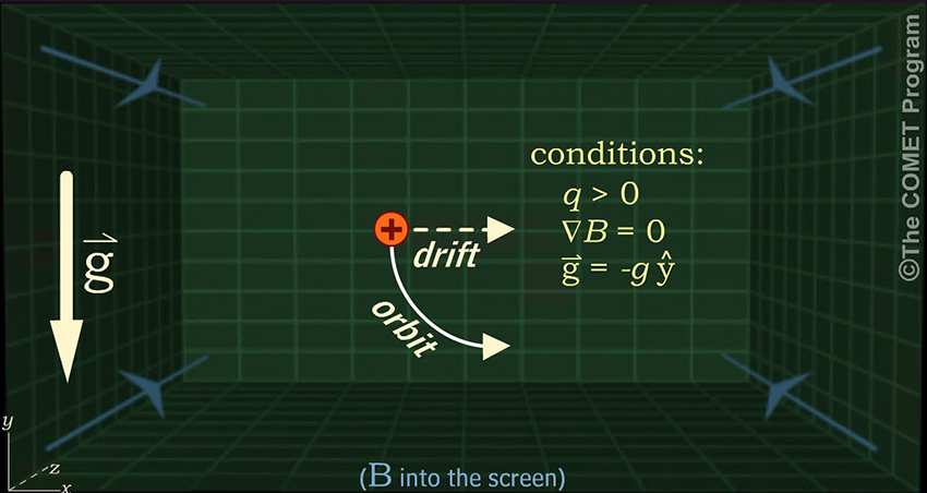
The proton orbits counterclockwise because the magnetic force on it is downward when it is moving to the left.
The proton drifts toward the right, because the downward gravitational force produces a maximum gyroradius at the bottom of its orbit, and this, combined with the counterclockwise orbit, produces an average drift to the right. An electron would drift toward the left because it orbits in the opposite direction, but the downward gravitational force would produce a maximum gyroradius at the bottom of its orbit.
Particle Drift Questions
-
If charged particles collide with neutral atoms and molecules, their drifts are necessarily modified.
Question 1
Consider the simple case where, on the average, collision with a neutral leads to a charged particle at rest. In the absence of collisions, what would be the trajectory of a positively charged particle initially at rest in uniform electric and magnetic fields, such that
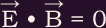 and
and  ? (Note that it is possible
to transform to an inertial frame moving at velocity
? (Note that it is possible
to transform to an inertial frame moving at velocity 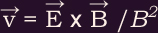 where
where  . )
. )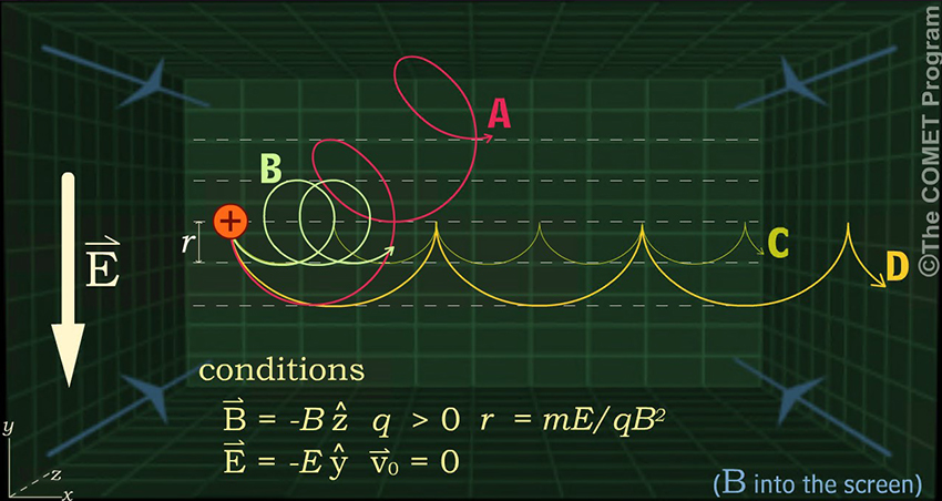
Given these conditions, what trajectory will the proton follow?
(Choose answer from the dropdown box, then click Done.)
In the rest frame where the electric field vanishes, the particle has a speed Of E/ B and travels in a circular orbit Of radius r = mE/qB2. In the original rest frame, we combine the linear motion (with speed E/ B) and the circular motion to produce trajectory D."
So long as (E/B)2 << c2, Where c is the speed of light, we can transform to a reference frame (moving with speed v = E/B to the right) in which the particle motion is simplified. In this reference frame, the electric field vanishes, the particle is initially moving with a speed v to the left, and the particle executes a circular orbit of radius r = mv/qB = mE/qB2, extending 2r below the initial particle position.
Knowing the particle motion in our new reference frame, we can transform back to the original frame and add the velocity vector of the orbiting particle to the transformation velocity, which has a magnitude v and is directed toward the right. The resultant velocity yields the particle trajectory D.
It is also possible to solve the time-dependent equation of motion for the particle in the original reference frame, and the same result is obtained.
Question 2
What happens when an ion's collision frequency is approximately equal to its gyrofrequency (
 )? What sort of trajectory will result?
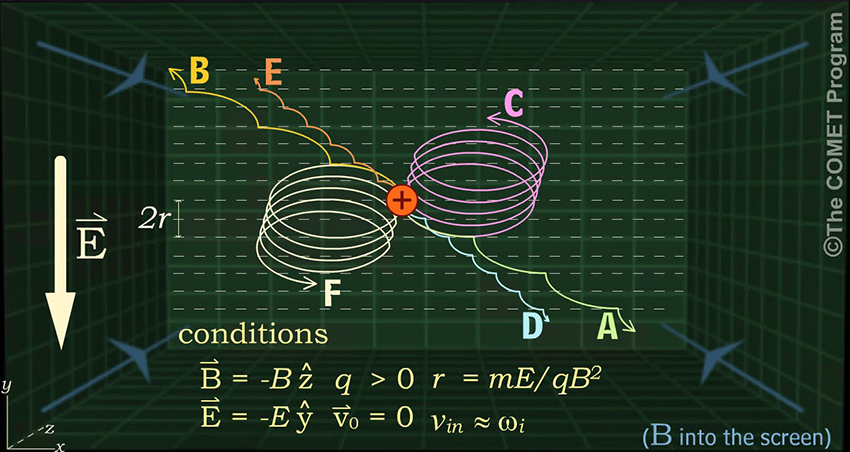
What trajectory will result at levels where collision frequencies ( Vin ) are approximately equal to ion gyrofrequencies ( ωi ) ?
(Choose answer from the dropdown box, then click Done.)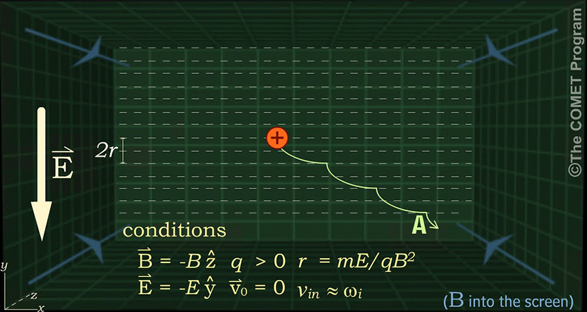
In situations where the collision frequency is approximately equal to a particle's gyrofrequency, a positively charged particle's drift trajectory will be similar to that of path A.
The conditions here are the same as in the preceding exercise, except that we have added collisions. If we assume that each collision (when Vin ≈ ωi) stops the particle after it has moved freely for about half a gyro-period, we can estimate our particle trajectory by taking a half gyro-period of the trajectory in the preceding exercise and repeating for each collision. This gives us trajectory A. Trajectories B, C, E, and F are incorrect, because in each case the particle drifts in the wrong direction. Trajectory D is in the right direction, but its gyro-radius is only half as large as it should be.
Question 3
In the E region of the Earth's ionosphere, ion and electron behaviors are very different. Ion collision frequencies are much greater than their gyrofrequencies (
 ); electron
gyro- and collision frequencies are the opposite (
); electron
gyro- and collision frequencies are the opposite ( ). What sorts
of currents do the resulting drifts generate?
). What sorts
of currents do the resulting drifts generate?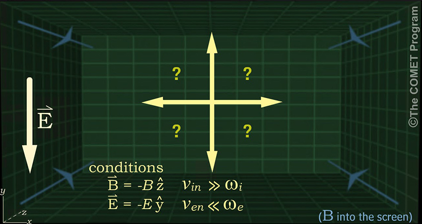
What drifts and currents will occur under the above conditions?
(Choose answer from the dropdown box, then click Done.)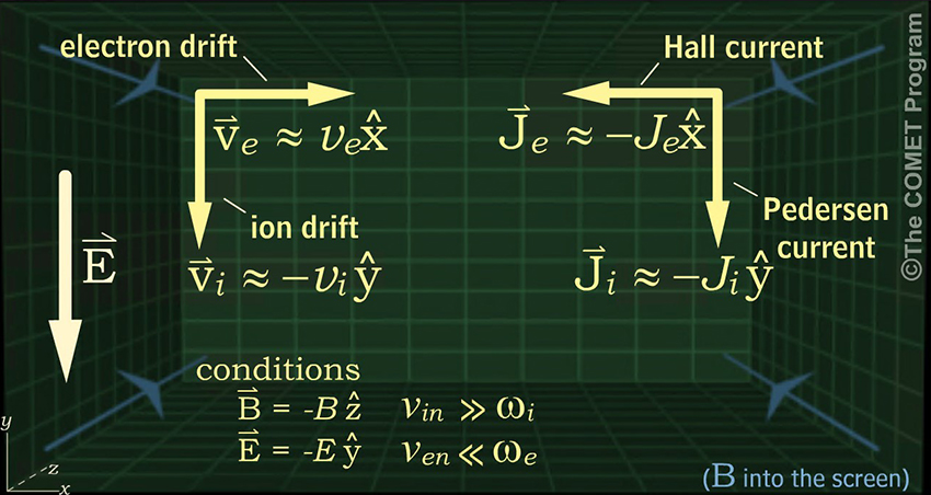
Hall currents are generated in the E-region of the Earth's ionosphere, where collision frequencies for electrons are much smaller than their gyrofrequencies. Pedersen currents are generated by ions, which collide with neutral particles at much higher frequencies than their frequency of gyration.
In this example, the electrons execute many gyroradii before they collide, while the ions travel only a fraction of a gyroradius before they collide (the electron-neutral and ion-neutral collision rates are comparable, but the electron gyrofrequency is some ten thousand times larger than the ion gyrofrequency).
Since the electron collision rate is very low, they end up drifting in the ExB direction, along the X-axis. The ions, on the other hand, collide so frequently (with neutral particles) that they never make it a significant distance around their gyro-orbit. As a consequence, they travel in the direction of the electric field, which keeps accelerating them downward after each collision.
Particle Drifts and Collisions
-
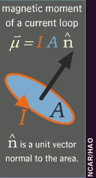
The magnitude of the magnetic moment
 , of a current loop with current
  and area
  is
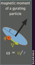
is  . A charged particle (in a magnetic field) moving in a circular
orbit forms a current loop with current
. A charged particle (in a magnetic field) moving in a circular
orbit forms a current loop with current 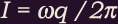 and area
  . From these, we can derive the
magnitude of the magnetic moment. (Click the question marks to see the derivation.)
. From these, we can derive the
magnitude of the magnetic moment. (Click the question marks to see the derivation.)
If the magnetic field does not change significantly during one gyroperiod, the magnitude of the magnetic moment remains constant, even as the particle moves into regions of different magnetic field strength.
The kinetic energy of the particle
 also remains constant, since the magnetic field does no work on the
particle. Defining the particle's pitch angle,
also remains constant, since the magnetic field does no work on the
particle. Defining the particle's pitch angle, 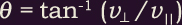 , we can apply the magnitude of the magnetic moment equation to
calculate a particle's trajectory for a given field. (Click the question marks to
see the derivation.)
, we can apply the magnitude of the magnetic moment equation to
calculate a particle's trajectory for a given field. (Click the question marks to
see the derivation.)
Magnitude of the Magnetic Moment and Particle Trajectories
-
The equation in the Magnitude of the Magnetic Moment and Particle Trajectories section tells us how a particle's pitch angle increases as it moves into a region of stronger magnetic field and decreases as it moves into a region of weaker field.
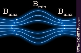
In a simple magnetic mirror geometry the magnetic field reaches a minimum value at the center of the geometry and a maximum value at the end. Particles within such a geometry can follow a range of trajectories, as described below.
Stuck in the Center
A particle with pitch angle
 cannot move into a region of stronger magnetic
field, so a particle with
cannot move into a region of stronger magnetic
field, so a particle with  (at the center of
the magnetic mirror, where B = Bmin) cannot move away
from the center of the mirror.
(at the center of
the magnetic mirror, where B = Bmin) cannot move away
from the center of the mirror.Straight and Narrow
On the other hand, a particle with pitch angle
 is free to move
anywhere and readily travels out of the magnetic mirror.
is free to move
anywhere and readily travels out of the magnetic mirror.Trapped in the Mirror
In a magnetic mirror geometry, particles with pitch angles in the following range are trapped within the magnetic mirror:
![theta-minimum > sin to the -1 [(B-min / B-max) to the 1/2]](./media/graphics/math/theta_min_gt_sin_minus_one_.jpg)
Into the Loss Cone
However, particles with
![theta-minimum < sin to the -1 [(B-min / B-max) to the 1/2]](./media/graphics/math/theta_min_lt_sin_minus_one_.jpg) are said to be in the loss cone and can
escape the magnetic mirror.
are said to be in the loss cone and can
escape the magnetic mirror.
Magnetic Moment and Mirroring
-
How will particles with different pitch angles behave within a magnetic mirror geometry?
Question
Match the pitch angles (Θmin) with the particle trajectories.
Four different ion trajectories are shown for the smae magnetic mirror field below. What are the corresponding pitch angles? Use the dropdown boxes to choose a particle trajectory for each pitch angle (at the center of the mirror geometry). When finished, click done.
Trajectory A
Trajectory B
Trajectory C
Trajectory D
Magnetic Mirroring Exercise
Magnetic Force
-
As shown in the Charged Particle Motions section, the magnetic force
 on a
particle is:
on a
particle is:This magnetic force equation can be combined with the current density equation to derive the magnetic force density per unit volume. Current density J is equal to ni qi ui + ne qe ue, where n is the particle density (ion or electron), q is the charge, and u is the average particle velocity. (Watch the video below to see the derivation.)
Magnetic Force Density
-
Ampère's Law tells us that
 (
( is the permeability of free space). We can apply this law to the the magnetic force
density equation to derive two important terms, magnetic tension
force and magnetic pressure gradient force. (Watch the
video below to see the derivation.)
is the permeability of free space). We can apply this law to the the magnetic force
density equation to derive two important terms, magnetic tension
force and magnetic pressure gradient force. (Watch the
video below to see the derivation.) The magnitude of the first term, the magnetic tension force, is twice the magnetic energy density divided by the radius of curvature of the magnetic field. The second term, the magnetic pressure gradient force, is minus the gradient of the magnetic energy density (or pressure).
Magnetic Tension and Pressure Gradient Forces
-
As shown on the preceding pages, the magnetic force density is equal to the magnetic tension force plus the magnetic pressure gradient force:

Whenever the current density vanishes
 the field becomes potential
  , and the
magnetic tension and pressure gradient forces must balance
, and the
magnetic tension and pressure gradient forces must balance  .
.
Magnetic Force Balance
-
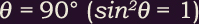
When applied to a plasma (i.e., an ionized gas) Newton's Second Law requires that the time rate of change of plasma momentum density
![[ d(ro u / dt)]](./media/graphics/math/d_ro_u_over_dt.jpg) equals the sum of the force densities acting on the plasma:
equals the sum of the force densities acting on the plasma: 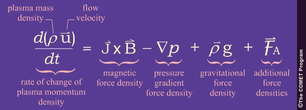
Plasma Momentum Balance
-
The magnetopause separates a region of relatively strong magnetic field (the magnetosphere) from a region of relatively weak magnetic field (the magnetosheath). What current is required to maintain a force balance across this boundary?
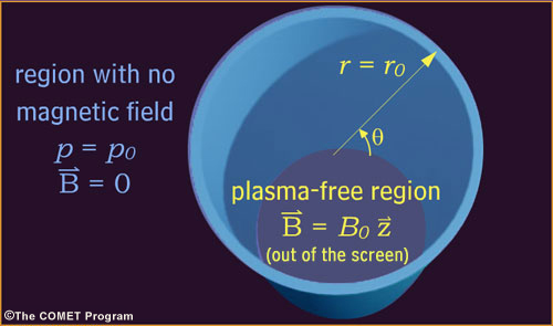
Consider a simplified case in which there is an equilibrium between a magnetic field contained in a cylindrical volume (aligned with the cylinder axis) surrounded by plasma at rest (u = 0). There is no plasma inside the boundary r = r0 and no magnetic field outside of it.
Questions
In the equilibrium illustrated above, the force balance involves only the plasma and magnetic pressure gradient forces
![[Grad (p + B-squared / 2 mu-sub-0) = 0]](./media/graphics/math/grad_p_plus_B2_over_2_mu_eq.jpg) .
.Question
Define the boundary current
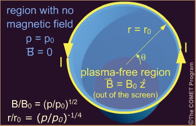
In the equilibrium (μ = 0) illustrated below, a magnetic field contained in a cylindrical volume (aligned with the cylinder axis) is surrounded by plasma. There is no plasma inside the boundary r = r0 and no magnetic field outside of it. Yhe force balance involves only the plasma and magnetic pressure gradient forces:
What current per unit length flowing around the cylinder of magnetic field is required to maintain this equilibrium? (Choose the best answer below. When finished, click Done.)
The correct answer is g).
The current per unit length flowing around the cylinder is obtained by integrating Ampere's Law:
∇ x B = μ0J
Across the boundary between the two regions:
I = -(B0/μ0)Θ
Question
Define the changes
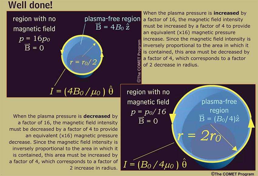
What happensto the equilibrium illustrated at right (and in the preceding exercise), when the plasma pressure is increased or decreased by a factor of 16?
(Choose the best answers below. when finished, click Done.)
If the plasma is increased by a factor of 16 (p = 16p0) how will the magnetic field (B) of the cylinder be affected?
The correct answer is a).
Question
If the plasma is increased by a factor of 16 (p = 16p0) how will the radius of the cylinder (r) be affected?
The correct answer is d).
Question
If the plasma pressure is decreased by a factor of 16 (p = p0 /16) how will the magnetic field (B) be affected?
The correct answer is b).
Question
If the plasma pressure is decreased by a factor of 16 (p = p0 /16) how will the current (I) be affected?
The correct answer is b).
Equilibrium Currents
-
Magnetic Flux Tubes
A magnetic flux tube encloses a single set of field lines. The surrounding surface is defined by a closed contour, perpendicular to the magnetic field, that encloses these field lines.
Like a fluid element (described in the Static Atmospheres section) a magnetic flux tube can be distorted, but never broken as long as the magnetic field lines keep their "identity" and the flux tube remains frozen to the ambient plasma.
In other words, a flux tube remains intact as long as:
- The magnetic flux enclosed by the contour remains constant if the contour moves with the plasma.
- All plasma initially lying along a magnetic field line continues to do so.
The frozen-field theorem (comprising these two conditions) is valid if
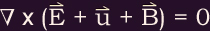 , where
  is the plasma flow velocity, and and are the
electric and magnetic fields.
is the plasma flow velocity, and and are the
electric and magnetic fields. (NOTE: The flux tubes in these illustrations appear to be discrete. In reality, magnetic fields do not vanish outside a flux tube as shown.)
Frozen-Field Theorem
-
Validity of the Frozen-Field Theorem
To explore the validity of the frozen-field theorem we must consider the following generalized form of Ohm’s law for a magnetized plasma:
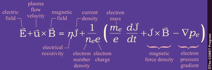
The first two terms in parentheses (
 and
and  )
arise from electron inertia and the Hall effect. The frozen-field theorem is
generally considered valid if the following conditions are satisfied, so that
)
arise from electron inertia and the Hall effect. The frozen-field theorem is
generally considered valid if the following conditions are satisfied, so that  :
: - The electrical resistivity is very small (
 ).
). - The current density is not too large.
- The spatial and temporal scales are not too small
- The electrical resistivity is very small (
-
Current Sheets
Although the frozen-field theorem is valid in most of the plasma regions we study, an important area where it breaks down is in current sheets. Current sheets are narrow regions of large current density (
 ). Ampere's Law ( ) tells us that a rapid spatial change in is a necessary
signature of such a sheet. Two examples of current sheets are shown below. Ampere's
law can be integrated across each interface boundary to deduce the currents flowing
in these sheets.
). Ampere's Law ( ) tells us that a rapid spatial change in is a necessary
signature of such a sheet. Two examples of current sheets are shown below. Ampere's
law can be integrated across each interface boundary to deduce the currents flowing
in these sheets.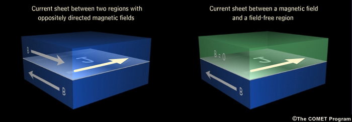
NOTE: The magnetic regions are illustrated as box-like spaces. In reality, magnetic fields are a continuum and cannot be confined in boxes. Thus the fields do not vanish outside the box edges as shown.
-
Question
According to the frozen-field theorem, a magnetic flux tube can be distorted but never broken as long as
. Under what circumstances does the frozen-field theorem
lose validity?
Question
Where is the frozen-field theorem invalid?
In the magnetic reconnection geometry shown below, the frozen-field theorem is assured valid everywhere except in one region. Which region is it?
(Choose the best answer. When finished, click done.)The correct answer is c).

If the plasma were frozen the field, there would be be a current sheet separating the oppositely directed magnetic fields and directed along the z-axis out of the screen. Even with a small resistivity, the large current density in a current sheet will produce resistive diffusion od plasma and magnetic field to form a finite-width current layer in the reconnection region.
-
The Fluid Element
Liquids and relatively dense gases such as the near-earth atmosphere, are generally treated as fluids. The basic building block of a fluid is the fluid element, an infinitesimal volume bounded by a closed surface that can be distorted but never broken:
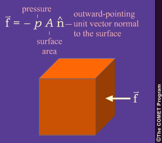
Fluid Pressure
The fluid has a pressure, p, expressed in units of force per unit area. The material surrounding a fluid element exerts a force on the fluid element's surface. In the simplest case, a fluid element shaped like a cube, the force on each face of the cube is:
Static Atmospheres
-
Pressure Gradient Force
If the pressure on a fluid element is uniform, there is no net force on the element. But variations in pressure generate net directional forces on a fluid element. For example, when pressure varies in the vertical ( z ) direction, with greater pressure, p1, below the fluid element and smaller pressure, p2, above it, a net upward force on the fluid element will result. (Watch the video below to see the derivation.)
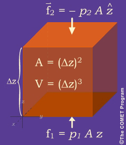
The pressure gradient force (
 ) is the force that supports a static atmosphere against downward
pull of gravity.
) is the force that supports a static atmosphere against downward
pull of gravity.
-
Tenuous Gasses
Although it is convenient to treat a dense gas as a fluid, the very tenuous gases found in the upper atmosphere, magnetosphere, and solar wind often require us to analyze the motions of the atoms and molecules (neutral and ionized) composing these gases. Here, we describe pressure and temperature of a gas in terms of the motions of its constituent particles.
Consider a relatively low-density gas inside a cubic container. A particle (such as an atom or molecule) with velocity
 striking the perfectly reflecting right
face of the cube rebounds with velocity
striking the perfectly reflecting right
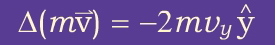
face of the cube rebounds with velocity  . If the particle has mass m, the change in
its momentum is:
. If the particle has mass m, the change in
its momentum is: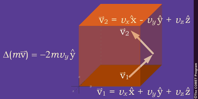
-
Gas Pressure & Temperature
As shown on the preceding page, when a particle rebounds from its containing cube wall, the change in its momentum (along the
 axis) is:
According to Newton's second and third laws, this change in momentum corresponds to an impulse
 exerted by the particle on the face of the cube.
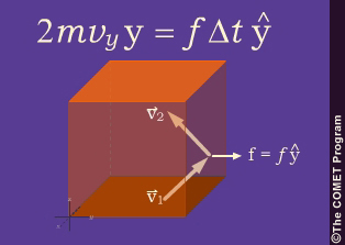
If half of the particles in the container are moving to the right at speed vy, and the particle density is n, then the number of particles per unit time striking the right cube wall with area A is ½nvyA. The resulting force per unit area, or pressure, on that face can then be derived as shown below. (Watch the video below to see the derivation.)
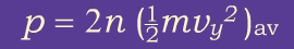
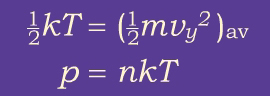
Since in reality not all particles in the container have speed vy , we replace vy2 with its average value, (vy2)av and express the pressure in terms of the average kinetic energy (½mvy2)av associated with motion along the y axis:
If we now define the temperature T to be proportional to the average kinetic energy, and take the proportionality factor to be one-half the Boltzmann constant, k, we can write:
The units of the absolute temperature we have just defined are known as Kelvins, represented by the letter K. The size of a Kelvin is the same as that of a degree Celsius, but the zero points of the Kelvin and Celsius scales are different: 273 K = 0ºC.
-
Gas Pressure & Temperature Questions
Refine your understanding of temperatures and pressures of tenuous gasses by answering the following questions.
Question
Compare solid and imaginary cubes
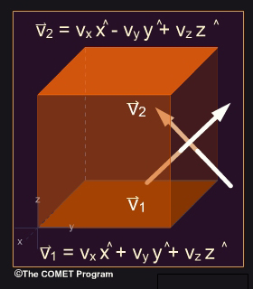
The Tenuous Gasses and the Gas Pressure & Temperature sections show how to derive the pressure of a tenuous gas by evaluating the force on the face of a cubic container from which the gas particles rebound.
Now consider the imaginary cube, which has no effect on the gas particles. Particles pass through the cube faces instead of bouncing off them. Think about two particles: As the first particle (v1) exits the cube across the right face, the second particle (v2) simultaneously enters the cube across the same face. How would momemtum and pressure differ? (Choose the best answer below. When finished, click Done.)
Compared to a solid cube, what change of momemtum in the y direction (inside the cube) results when particle 1 exits the cube while particle 2 enters it?
The correct answer is b).
Question
What would be the corresponding pressure?
The correct answer is b).
Momemtum changes the pressure are the same in both the solid and imaginary cubes. Particle v1 carries momentum mvyy out of the cube, so it contributes Δ(mv) = -mvyy to the cube. Particle v2 carries momentum -mvyy into the cube, so it also contributes Δ(mv) = -mvyy to the cube.
The net contribution is Δ(mv) = -2mvyy, which is the same as before. Once this result is obtained, the same reasoning used before leads to the same result for the pressure of the gas: p = nkT
-
Force Balance and Scale Height
In a static atmosphere whose constituents are electrically neutral atoms and molecules, the atmospheric structure is governed by a balance between the downward gravitational force and the upward pressure gradient force. This balance is described by the equation dp/dr = -nmg. Recalling that p = nkT, we can divide the force balance equation by the pressure to obtain the pressure scale height. (Click the question marks to see the derivations.)
-
Scale Height Differences
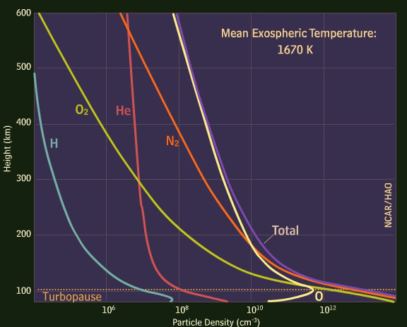
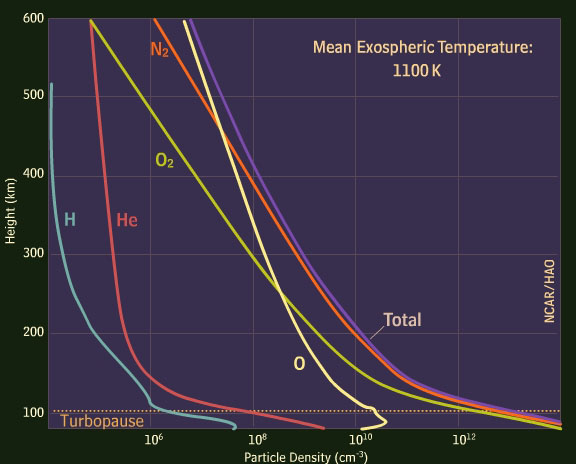
The equations on the previous page can be used to calculate density-height profiles for the different constituents of upper atmospheres where gasses are tenuous and there is little turbulent mixing. Consider the following equations:
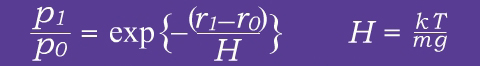
When r1- r0 = H, the equation on the left reduces to:
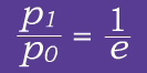
So, scale height is the height range over which the pressure decreases by a factor of e (2.718...). For higher temperatures and smaller particle masses, the scale height is larger and the pressure drops off more slowly with height.
You can see these differences in the below two density-height plots. The upper plot was calculated for a mid-level (300-400 km altitude) temperature of 1670° K, while the lower one was plotted for an 1100° K temperature.
Watch the video below to view the full interactive diffusion simulation.
-
Force Balance Exercise
Refine your understanding of force balance and scale height by answering the following questions.
Question
Consider an atmosphere composed of oxygen and helium atoms, which both have the same temperature. Assume that there is no atmospheric mixing, so that each constituent attains its own scale height. Now answer the following questions comparing oxygen and helium in such an atmosphere.
(Choose the best answer for each drop-down box. When finished, click done.)The scale height varies inversely with the particle mass, and the atomic mass of oxygen is four times that of helium, so the helium scale height is four times larger than the oxygen scale height. Since a larger scale height corresponds to a slower pressure (or density) decline with height, the pressure and density of oxygen decline more rapidly than those of helium. If the oxygen scale height is H(O) = 100 km, then the helium scale height is H(He) = 400 km
If the scale heights are constant throughout the height range we are considering, and if the He/O density ratio is 2 at 300 km, then at a distance Δr above 300 km, the density ratio will be 2 exp (-Δr / 100 + Δr / 400). Thus the density ratio is 1 when Δr = 92, which corresponds to a height of 392 km.
-