9.6 Forecast Verification and Validation »
9.6.2 General Methods for Forecast Verification »
9.6.2.6 Methods for Verification of Ensemble Forecasts
As we discussed in Section 9.4.5Section 9.4.5, ensembles consist of many versions of a single dynamical model or many different dynamical models. The ensemble forecast captures the uncertainty in the forecast and provides a range of outcomes.
Many methods for evaluating probability forecasts can also be implemented for evaluating ensemble forecasts, where the spread of the ensemble members indicates probability. However, since ensembles provide information on the range of possible outcomes given the particular initial conditions, other measures of skill can also be applied to ensembles. We review just a few. You are encouraged to explore further using the cited references and resource links.
- Rank histogram The rank histogram is a quantitative, multi-category method of verification that is represented visually (e.g., Fig. 9.82). It measures how well the ensemble spread of the forecast represents the true variability (uncertainty) of the observations. It is also known as a “Talagrand diagram”.116,117
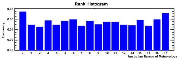
In an ensemble with perfect spread, an observation is equally likely to fall between any pair of ensemble members since each ensemble member represents an equally likely scenario. Therefore, we can evaluate the success of the ensemble spread by looking at the shape of the rank histogram. If the histogram is:
- Flat, the ensemble spread is acceptable for representing the forecast uncertainty. Note that a flat rank histogram does not necessarily indicate a good forecast, only that the ensemble is a reasonable representation of the observed probability distribution;
- U-shaped, the ensemble spread is too small since many observations fall outside the range spanned by all of the ensemble members.
- Dome-shaped, the ensemble spread is too large since most observations fall near the center of the range of the ensemble set;
- Asymmetric, the ensemble has an overall bias compared to observations.
Verifying forecasts of rare and/or extreme events
Since we are interested in verification for ensemble forecasts of TC, we will briefly review two methods for verifying ensemble forecasts of rare and extreme events.
- Deterministic limit
The deterministic limit118 is the forecast lead time at which the number of misses plus false alarms in the ensemble forecast set equals the number of hits for a chosen weather system. It measures the forecast lead time for which the forecast is more likely to be correct than incorrect (Fig. 9.83). While this may not sound too exciting, it could help the forecaster to decide how much weight to give that forecast and, possibly, to decide to switch from deterministic to probabilistic guidance.
One example of the use of a deterministic limit would be the statement that “The deterministic limit for forecasts of TC intensity by the XXX model is 24 hours.”
- Extreme Dependency Score
The Extreme Dependency Score (EDS) measures the reliability of a model to forecast a specific weather system, such as a TC. The EDS119 is a measure of the forecast skill for observed rare events. It ranges between -1 and 1, where a perfect score is EDS=1.
http://www.dtcenter.org/met/users/index.php
Statistical challenges for verification of forecasts of weather extremes,
http://www.cawcr.gov.au/projects/verification/Casati/statxtr.htm
9.6 Forecast Verification and Validation »
9.6.3 Summary: Advantages and Inadequacies of Current TC Forecast Models
Based on results from the current verification methods, we can make some general comments on the skill of the current generation of forecast models.
While it is possible for the human forecaster to show skill over the operational forecast models from time to time, model performance has improved significantly over the years, and they are now very difficult to beat on a consistent basis, at least for track forecasts.
Intensity forecasting is much more complex than track forecasting. For a start, intensity forecasts rely in some measure on the track forecasts (e.g., to get interactions with other weather systems and SST information). Further, intensity depends on details of the TC core structure, such as the distribution of deep convection, and other internal storm processes. Thus, dynamical forecast models still have little skill in predicting TC intensity change.
Statistical models for TC intensity are beginning to provide useful guidance, although since they are built using historical storm information, their skill is restricted to “typical” TC intensity evolution. Events such as rapid intensity change are not well forecast in either statistical or dynamical models. Current statistical models of rapid intensity change are based on a very small set of storms, which limits the range of possible intensity changes that underlie the statistical model.
Consensus forecast systems offer hope for improvements in forecast accuracy. Ensemble prediction systems are beginning to address the problem of TC forecasting directly101,120 by targeting TC when the ensemble perturbations are developed,80 rather than developing the perturbations as part of a larger forecasting problem. These offer hope of improved forecasts, not only of TC track and intensity, but on wind and rainfall distributions and storm structure evolution. Forecasting of extratropically transitioning TC121 (ET, Section 8.5ET, Section 8.5) and the influence of these ET systems on the midlatitude flow122,123 is also a critical problem being studied using these targeted model ensembles.
Focus Areas
Focus Areas »
Focus 1: The Australian-Indonesian Monsoon
Focus 1: The Australian-Indonesian Monsoon »
9F1.1 Overview of the North Australian Monsoon
by Dr. Mick Pope of the Australian Bureau of Meteorology (BoM)
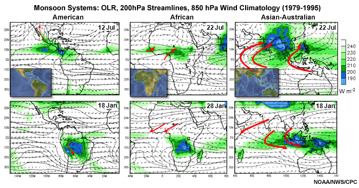
The monsoon refers to the tropical and subtropical seasonal reversals in the atmospheric circulation and associated precipitation,124 leading to two distinct phases, “wet” and “dry” (Fig. 9F1.1).125 The changes in the atmospheric circulations arise from reversals in temperature gradients between continental regions and the adjacent oceans. In many cases this is accompanied by the seasonal migration of the Hadley cell and associated monsoon trough or ITCZ. However, in the case of the American monsoons (Fig.9F1.1, left panels), no seasonal reversal of the winds has been identified.125 Equatorial regions have two rainy seasons and the trade wind flow collects moisture over the warm tropical oceans. In locations like Australia and India, one rainy season occurs when the cross equatorial flow turns westerly (Fig. 9F1.1, right panels). The corresponding trade wind easterlies are dry and characterized by a low-level inversion which caps deep convection.
This focus section will examine the Australian-Indonesian monsoon as a case study of monsoon dynamics, with a particular focus on the differences between the various intraseasonal phases.
Focus 1: The Australian-Indonesian Monsoon »
9F1.1 Overview of the North Australian Monsoon »
9F1.1.1 The Seasonal Cycle
Like the Indian monsoon,126 the Australian-Indonesian monsoon undergoes intraseasonal variation consisting of active and break phases, characterized by widespread and isolated precipitation respectively (Fig.9F1.2).

The NAM forms part of the global monsoon driven by the Hadley Cell. Up motion occurs in the hot towers due to condensational heating, resulting in lower pressures near the surface in the tropics and hence a cross equatorial pressure gradient with the winter hemisphere mid-latitudes. The column heating in the hot tower also produces a much stronger reverse pressure gradient in the upper troposphere which drives the upper return flow into the winter hemisphere.127 Modeling studies show that the response to the tropospheric heating is stronger when the heating is off the equator.128 Superimposed on this is the land-sea thermal contrast that develops during Austral Spring.125 A heat low develops over the Pilbara region, often resulting in shallow westerly flow over northern Australia, which moistens and pre-conditions the environment for deep convection (Fig.9F1.3). The period during which this pre-conditioning and isolated shallow convection occurs is known as the buildup. There is also a forcing due to the seasonal migration of the warmest sea surface temperatures.129
![]() A significant amount of rainfall occurs outside of the period of westerly winds. What weather systems would be responsible for this? We will answer this question in a later section.
A significant amount of rainfall occurs outside of the period of westerly winds. What weather systems would be responsible for this? We will answer this question in a later section.
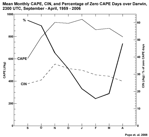
The seasonal cycle can also be considered in terms of the CAPE—a proxy for the strength of convective updrafts. The most energetic updrafts occur on average during November to January. Figure 9F1.4 shows the month values of CAPE, Convective Inhibition (CIN) and number of zero CAPE days for the 2300 UTC Darwin sounding. The amount of CAPE almost doubles during the late dry season (September through November), with a rapid decrease in the number of zero CAPE days. The increase in the CIN during this period is likely an artifact of the large number of zero CAPE days during September and October. Zero CAPE days reach a minimum at the peak of the monsoon during February, although this is not the time of maximum mean monthly CAPE.
Focus 1: The Australian-Indonesian Monsoon »
9F1.2 Regimes of the North Australian Monsoon
Focus 1: The Australian-Indonesian Monsoon »
9F1.2 Regimes of the North Australian Monsoon »
9F1.2.1 TWP-ICE
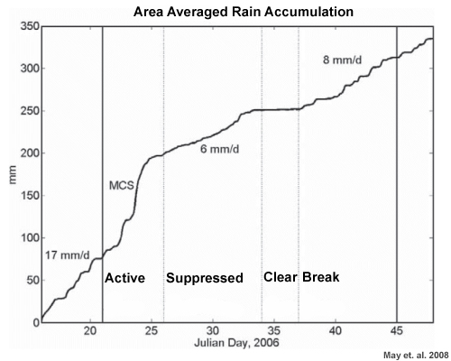
The NAM undergoes significant intraseasonal variability. Figure 9F1.5 shows the area average rain accumulation for January and February 2006 from the Tropical Warm Pool – International Cloud Experiment (TWP-ICE).131 The active period of the monsoon was marked by deep zonal westerly winds over Darwin and, during 23-26 January, an intense mesoscale convective system (MCS) produced an area averaged rainfall rate of approximately 45 mm day-1. The period starting February 6th is referred to as a break monsoon with deep tropospheric easterly winds, which produced an area averaged rainfall rate of approximately 8 mm day-1.
The NAM is characterized by active and break periods.132,133,134 During periods when the MJO is active (which it is not during all summers) there is a strong synchronization between the active-break cycle and the MJO.135,136 Likewise, the greatest probabilities of rainfall in the highest quintile are observed during the active MJO phase. Other influences on the monsoon at Darwin include upper troughs137 and equatorially-trapped Rossby wavesequatorially-trapped Rossby waves.138
The unusual phenomenon observed during TWP-ICE was the suppressed period of relatively small rainfall, together with the three days of clear conditions over Darwin with no rainfall. We now consider these three monsoon regimes in more detail.
Focus 1: The Australian-Indonesian Monsoon »
9F1.2 Regimes of the North Australian Monsoon »
9F1.2.2 The active monsoon

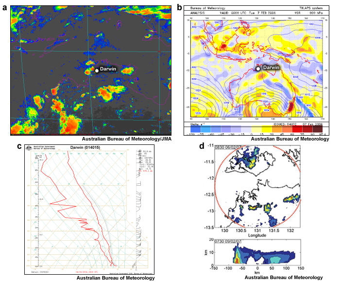
The active monsoon is associated with widespread, deep tropical convection, indicated by cold clouds in the IR image (Fig. 9F1.6a); although some cold clouds may be cirrus as IR cannot distinguish between precipitating convection and cold cirrus (Chapter 2, Section 2.5.2Chapter 2, Section 2.5.2). The associated synoptic pattern is a deep low over the Kimberley, directing west to northwesterly winds over northwest Australia and surrounding waters. The Monsoon Trough (MT) is indicated by the east-west oriented cyclonic vorticity maximum. Equatorward of the MT, the flow is converging into the low, resulting in the observed cloudiness and vertical motion profile (Fig. 9F1.6a,c). The sounding shows a typical active monsoon profile with a small dewpoint depression through the depth of the troposphere and a lapse rate close to moist adiabatic. The CAPE is typically small during the active monsoon. The wind profile is westerly to approximately 400 hPa with easterly winds above that. Drosdowsky (1984)139 defined the active monsoon in terms of the wind profile, with mean westerly zonal winds to 500 hPa and mean easterly zonal winds above 300 hPa.
Which weather elements are likely to be important in an active monsoon environment? What timing for the onset and cessation of these events might be appropriate and why? (Type your answer in box.)
Feedback:
Below is an example of the evolution of convective weather expected during an active monsoon; as expressed in a Terminal Aerodrome Forecast (TAF).
TAF YPDN 171802Z 1718/1818 34015KT 9999 SCT020
TEMPO 1718/1802 30020G40KT 1000 TSRA BKN010 SCT020CB
INTER 1802/1810 30020G40KT 3000 +SHRA BKN010
TEMPO 1810/1818 31020G40KT 1000 TSRA BKN010 SCT020CB
The Terminal Aerodrome Forecast (TAF) for Darwin shows periods of reduced visibility, lowered cloud base and precipitation in the form of heavy rain showers (+SHRA) and thunderstorms with rain (TSRA) throughout the validity period of the forecast which is 24 hours from 1800 UTC (0330 LST). An INTER means that conditions persist for periods of 30 minutes or less, a TEMPO for periods between 30 minutes and 1 hour.
During the thunderstorms described by the TAF above, the visibility is down to 1 km and in heavy showers to 3 km. The term BKN010 refers to low cloud with a base of 1000 feet, covering between 5 and 7 oktas (eighths) of the sky. The 24-hour coverage is consistent with the widespread cloud cover observed and the presence of synoptic-scale convergence and upward motion (Fig. 11F1.6). The focus of deep convection during the night and morning hours (between 1000 UTC = 1930 LST and 0200 UTC = 1130 LST) implies that deep convection is more likely to be nocturnal during the active monsoon, characterizing the airmass as maritime. The use of the TEMPO for this length of time is designed to include the time of potential enhanced convection and associated reduced visibility and cloud base due to the convection and enhanced by the wet bulb process. The peak in number and strength of updrafts does not typically occur until after dawn (about 0700 â 0900 LST).
Focus 1: The Australian-Indonesian Monsoon »
9F1.2 Regimes of the North Australian Monsoon »
9F1.2.3 The Break Monsoon
In contrast to the active monsoon, clouds are more isolated during the break periods (Fig. 9F1.7), often coastal, due to triggering on the sea breeze, and westward propagating. The MSLP/vorticity plot shows that the MT is to the north of Darwin, extending from the Arafura Sea into the Coral Sea. A region of cyclonic vorticity lies along the west coast of Australia extending into a heat low.
What differences do you observe between the trace (sounding) for the break monsoon period (shown below in 9F1.7c) ) and the active monsoon? (Type your answer in box.)
Feedback:
The main features of the sounding are easterlies through most of the troposphere compared to the westerlies of the active monsoon. The shallow westerlies near the surface are a result of the heat low. The zig-zag pattern in the dewpoint profile indicate dry air in mid-levels, referred to as dry slots.
Where on the satellite image, in Fig. 9F1.7, do you expect the sea-breeze front to be found over northern Australia? (Type your answer in box.)
Feedback:
Where on the satellite image do you expect the sea-breeze front to be found?
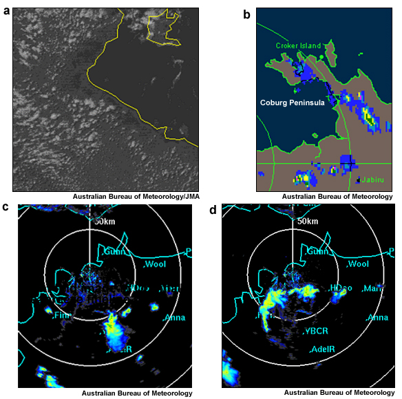
Convection usually occurs at the leading edge of the sea-breeze front,140 where the warm and moist inland air of the prevailing flow is lifted to its level of free convection. The orientation of the prevailing flow determines the preferred locations of convective development (Fig. 9F1.8). Convective rolls are also generated inland. The air mass coastward of the sea-breeze front is indicated by the cloud free region along the coast. On the radar image, the sea-breeze front is indicated by the line of convection parallel to the coast. Convection along the Coburg peninsula is indicative of the convergence of sea breezes (Fig. 9F1.8b).
The sea-breeze front also interacts with existing convection. In Fig. 9F1.8c, the sea-breeze front is seen as a light blue line oriented from Humpty Doo (HDoo) to Finnis Range (Finn). A thunderstorm propagates in from the southeast. Once the storm reaches the sea-breeze front, the outflow interacts with the sea breeze to initiate fresh convection, in this case, a squall line propagating to the northwest.
Compare the Darwin TAF for the break period (below) with the one for the active periodactive period. What differences do you observed for the wind? How does this relate to the differences in synoptic regime? What differences are observed in the key weather elements and timing?
TAF YPDN 061611Z 0618/1818 22007KT 9999 SCT020 FM0802 30014KT 9999 SCT030
TEMPO 0706/0612 10015G35KT 1000 TSRA BKN010 SCT020CB
(Type your answer in box.)
Feedback:
The winds are northwesterly in the active monsoon but here the wind is southwesterly turning northwest during the morning. Thunderstorms are forecast during the afternoon and evening, compared to showers and storms for the active monsoon. The TEMPO is diurnal rather than through the period, indicating that the trigger convection is due to the sea breeze and surface heating.
Focus 1: The Australian-Indonesian Monsoon »
9F1.2 Regimes of the North Australian Monsoon »
9F1.2.4 Comparison Between the Active and Break Periods
Given the mean diurnal cycle for the Australian-Indonesian monsoon shown in Section 5.3.7.2Section 5.3.7.2, what differences would you expect between the active and break periods for a place like Darwin?
(Type your answer in box.)
Feedback:
The active and break monsoon environments have different synoptic forcing and air masses. These differences should be reflected in the diurnal cycle of the resulting deep convection, as has been suggested by the TAFs of the activeactive and break break periods shown earlier. Figures 9F1.9 and 9F1.10 compare the diurnal cycles of convection for different phases of the monsoon.
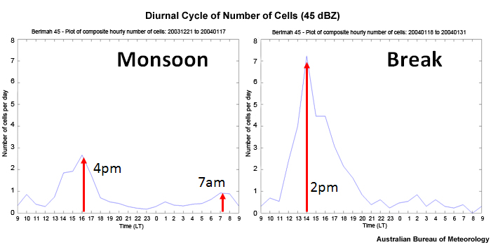
The break period has a strong diurnal signal, with a peak at 1400 LST. The timing of this peak is location dependent. It depends on the day to day synoptic forcing, sea-breeze cycle, and occurrence of earlier convection which may suppress the environment. The active period has a relatively flat diurnal cycle, with a weaker diurnal maximum at 1600 LST, compared to the break, and a morning peak at 0700 LST. The relatively flat diurnal cycle is consistent with the maritime nature of the air mass.
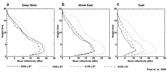
Another way to illustrate the diurnal cycle is to compare the mean reflectivity versus height (Fig. 9F1.10). The active monsoon has a very weak diurnal cycle with maximum values at 0930 and 1530 LST. The break period has a flat diurnal cycle except for the pronounced afternoon peak at 1530 LST when the mean reflectivity increases by 10 dBZ over most of the depth of the troposphere. The buildup profile is typical of the early wet season, when the surface moisture is still increasing. The echoes are not as deep as the break period or as large for a given height, indicating weaker updrafts. This is due to the entrainment of drier environmental air in the boundary layer. The gradual increase in reflectivity during the diurnal cycle is consistent with the mechanism by which multiple plumes moisten the atmosphere and allow larger rain droplets to form.
![]() What differences will the amount of convection make to the thermodynamics of the active and break regions and vice versa?
What differences will the amount of convection make to the thermodynamics of the active and break regions and vice versa?
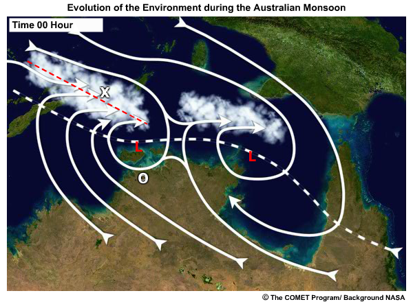
Active or break environments occur relative to the monsoon trough, as shown in Fig. 9F1.11. In the southeasterly stream poleward of the monsoon trough at O, dry air advection results in the dry slots observed in the dewpoint profile. Equatorward of the monsoon trough at X, moist maritime air is lifted in the convergent region to produce a deep moist profile. Fig. 9F1.11 illustrates that, as the monsoon trough migrates poleward, winds shift from easterly to northeasterly with southeasterly flow in the upper troposphere to deep monsoon westerly with easterly flow aloft. Tropospheric moisture increases with the change in trajectories and synoptic forcing.
Time 00 Hour
Click the O to see an aerological profile. Click the X to see a cross section animation.
Time 12 Hour
Click the O to see an aerological profile.
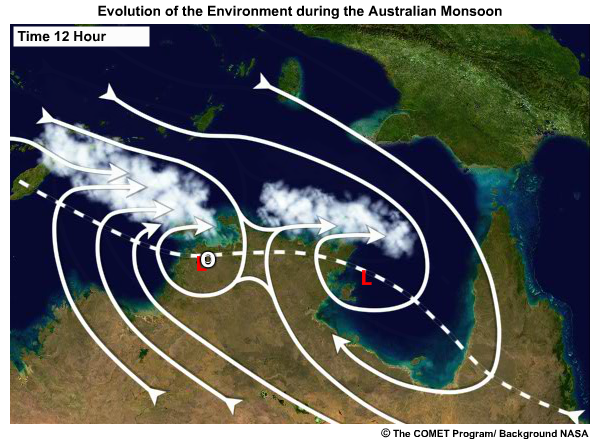
Time 24 Hour
Click the O to see an aerological profile.
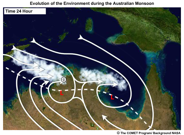
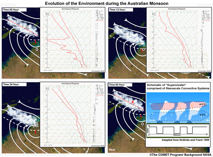
The cross section (shown by clicking the X on the image in the Time 00 Hour tab of Fig. 9F1.11) illustrates the difference in CAPE and lapse rate between the active and break period environments. Latent heat release in the mid to upper troposphere warms the environment while evaporation of precipitation cools the lower troposphere, stabilizing the lapse rate. Spreading near surface cold pools reduces the CAPE by bringing down cooler and drier air from aloft. During break periods, shortwave heating of the surface and longwave cooling of the atmosphere destabilize the troposphere and allow CAPE to recover.
Focus 1: The Australian-Indonesian Monsoon »
9F1.2 Regimes of the North Australian Monsoon »
9F1.2.5 The Suppressed Monsoon
Refer back to Fig 9F1.5. What kind of synoptic environment could produce a suppressed regime?
(Type your answer in box.)
Feedback:
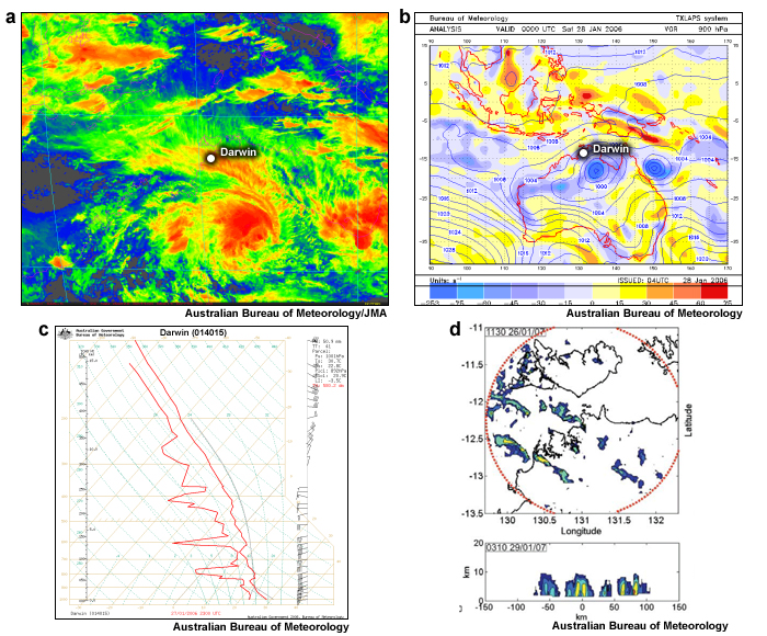
The suppressed monsoon over Darwin is due to a deep low over central Australia (Fig. 9F1.12). Such deep lows are referred to colloquially as ‘landfoons’ due to their structural similarity to tropical cyclones (also known as typhoons) in the satellite imagery and their potential to become tropical cyclones were they over the warm, tropical ocean.143 The MSLP/vorticity chart shows that the monsoon trough is well to the south of Darwin, together with the associated convergence. The flow is southwesterly rather than the west to northwesterly flow associated with an active monsoon.
Compare the trace (sounding) of the suppressed monsoon to the trace for the active monsoon. How is the wind profile similar/different? How is the dewpoint profile different?
(Type your answer in box.)
Feedback:
The winds are strong westerly as is the case for the active monsoon, but the meridional component is southerly. The ‘dry slots’ in the dewpoint profile look like those in the break period monsoon profile. The suggestion is that the trajectories are different due to the location of the low; advecting drier air from further south. Examination of model moisture fields and backward trajectories confirms this.
What differences will the drier trajectories produce in the Darwin? Is deep convection likely?
(Type your answer in box.)
Feedback:
Below is a description of the weather situation including an example TAF.
TAF YPDN 271613Z 2718/2818 27020G30KT 9999 BKN020
INTER 2718/2818 26020G40KT 4000 SHRA BKN010
The TAF indicates an INTER (less than 30 minutes at a time) showers only which indicates a relatively suppressed environment, i.e., no deep convection. Note that Fig. 9F1.5 indicates that, as the low moved further south, conditions became more suppressed so that eventually no showers were observed.
The occurrence of the suppressed monsoon highlights the shortcomings of zonal wind only based definitions of monsoon onset. More work is required to more rigorously define the regimes of the NAM.141
Focus 1: The Australian-Indonesian Monsoon »
9F1.2 Regimes of the North Australian Monsoon »
9F1.2.6 Summary of NAM Regime Differences
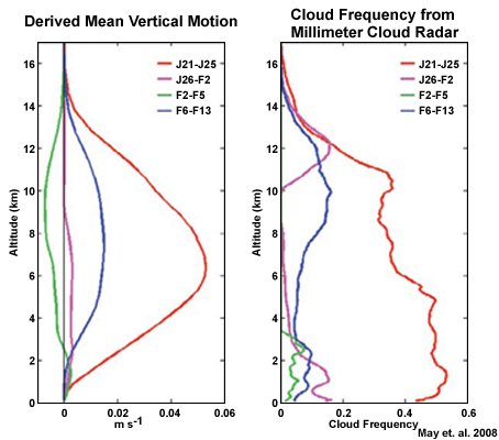
The active monsoon is dominated by deep upward motion, reaching a maximum near 6 km, and a large cloud frequency (red line in Fig. 9F1.13). Although the break monsoon period contains some intense storms, their isolated nature and differences in the large scale forcing means that the mean vertical motion is much less than the active monsoon (blue line in Fig. 9F1.13). The suppressed monsoon has very weak mean vertical motion, and the vertical cloud frequency profile shows the prevalence of shallow convective cloud mostly below 3 km, together with the cirrus between about 10 and 14 km. The cloud free period is unsurprisingly associated largely with subsidence.
Focus 1: The Australian-Indonesian Monsoon »
9F1.3 Storm Types of the North Australian Monsoon
This section examines some of the convective weather systems associated with the NAM. It is not an exhaustive treatment.
Focus 1: The Australian-Indonesian Monsoon »
9F1.3 Storm Types of the North Australian Monsoon »
9F1.3.1 Wet Microbursts
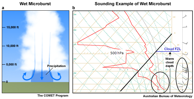
A wet microburst is a thunderstorm which produces damaging surface winds associated with significant precipitation at the surface and a low cloud base (Fig 9F1.14). Typically, the moisture extends to about 500 hPa with a dry layer above and the wind shear is weak. The low cloud base is due to high relative humidity near the surface, inhibiting evaporation. A warm cloud depth of greater than 10000 ft allows the collision and coalescence process to produce large rain drops. These conditions imply that precipitation drag is important in forming the downdraft. These storms occur during active and break monsoon conditions.
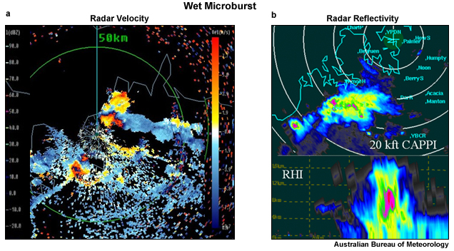
On 31 January 2000 wind gusts of 100 and 150 km h-1 were produced by a sustained wet microburst of about 30 minutes in duration. Figure 9F1.15 shows the Doppler velocities for a wet microburst. Figure 9F1.15 also shows the effect of large CAPE on a wet microburst environment. Large CAPE result in strong updrafts which produce elevated strong reflectivity echoes, making it possible to detect an impending downburst before it occurs. For small to moderate CAPE (< 2000 J kg-1) the first echoes are observed at about 3–6 km (10–19000 ft). These typically produce non-severe wind gusts. For larger CAPE, first echoes are observed at about 7–9 km (22000–30000 ft).
Focus 1: The Australian-Indonesian Monsoon »
9F1.3 Storm Types of the North Australian Monsoon »
9F1.3.2 Dry Microbursts
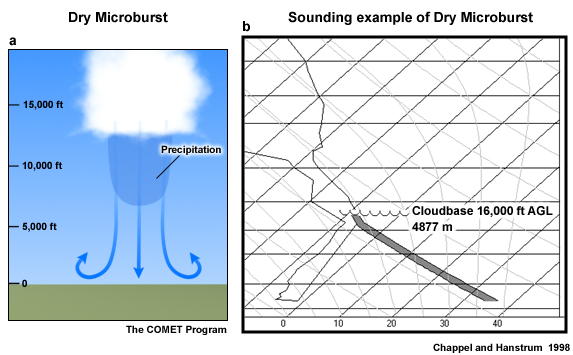
Dry microbursts are a feature of inland Australia in an environment of deep easterly flow where the boundary layer is deep (up to 16000 ft above ground level) and dry. These storms produce damaging winds at the surface with no precipitation. Updrafts are weak due to low CAPE and vertical wind shear is weak. Hence, the downburst is produced by evaporation. The trace shown in Figure 9F1.16 was observed at Alice Springs aerodrome in 1992, and produced wind gusts of 72 and 94 km h-1. These storms are difficult to forecast because mixing with the hot environmental air and weakens the negative buoyancy of the downdraft. These storms occur during active and break monsoon conditions.
Focus 1: The Australian-Indonesian Monsoon »
9F1.3 Storm Types of the North Australian Monsoon »
9F1.3.3 Continental Squall Lines
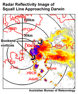
Continental squall lines occur during break phases of the monsoon and can produce potentially damaging surface winds. A typical continental squall line, approaching Darwin from the east, consists of a leading edge of deep convection with a trailing stratiform region (Fig. 9F1.17).
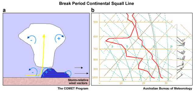
The basic conceptual model of a squall line is a line of convection propagating perpendicular to the mean wind shear vector or mean steering flow (COMET’s Convective Storm Matrix). The strong unidirectional wind flow provides wind shear to balance the vorticity generated at the leading edge of the spreading cold pool by buoyancy gradients to generating new convective cells at the leading edge (Fig. 9F1.18). The wind profile also provides winds to ingest in the convective downdraft as surface gusts. The cold pool is produced by the evaporation of precipitation falling through unsaturated environmental air, known as the dry slot.
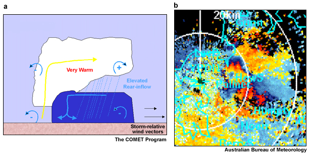
One of the signatures of a severe squall line is the rear inflow jet. Strong rear inflow jets occur in large CAPE, strong vertical wind shear environments. The rear inflow jet accelerates the flow into the rear of the squall line and hence increases the potential surface wind gusts.
Eventually, the cold pool outruns its parent convection and the squall dies. At this stage, the strongest surface winds occur as the rear inflow jet reaches the surface in the downdraft (Fig. 9F1.19). Evidence of a rear inflow jet and imminent surface wind gusts can be obtained from Doppler radar. Fig. 9F1.19 shows Doppler imagery with double range folding to 25 m s-1 (~ 50 kts) 9 minutes before the measured gust of 58 knots at the surface. A thin region of dark blue indicates this range folding, moving through orange shades and then through again to dark blue "circular" regions.
Another feature of potential severity for squall lines is the bookend vortex. Bookend vortices result from vorticity at the leading edge of the cold pool being lifted and tilted by the updraft (reference). The bookend vortices can increase the strength of the rear inflow jet and cause part of the squall line to bow outwards as a bow echo. Figure 9F1.17 shows a bow echo, as well as curved elements in the reflectivity at either end of the leading edge, indicative of bookend vortices.
Focus 1: The Australian-Indonesian Monsoon »
9F1.3 Storm Types of the North Australian Monsoon »
9F1.3.4 Monsoon Squalls
A monsoon squall, also referred to as maritime squalls, form in an environment of deep westerly winds. The lines occur in regions of moderate to strong wind shear in the lower troposphere, and with a block of strong westerly winds. Figure 9F1.20 shows an example of a series of linear features with strong surface winds moving over the Tiwi Islands. A large dry slot exists between 800 and 500 hPa. One monsoon squall on 3 January 2005 produced several convective lines resulting in gusts observed up to 110 km h-1.

Focus 1: The Australian-Indonesian Monsoon »
9F1.4 The Monsoon over the Maritime Continent
Focus 1: The Australian-Indonesian Monsoon »
9F1.4 The Monsoon over the Maritime Continent »
9F1.4.1 Hector and Convection over Flat Islands
Hector is a thunderstorm complex occurring over the Tiwi Islands, with a height > 15 km, and a horizontal extent of the > 30 dBZ echo of at least 200 km2.145 Hector forms during the break periods of the monsoon. The zonal tropospheric wind flow during this period is easterly, providing the steering flow as is the case for tropical squall lines. The direction of the low-level flow determines where convective initiation starts (Fig. 9F1.21). Figure 9F1.21 also shows the evolution of Hector when the low-level flow is westerly, such as occurs when there is an active heat low over mainland Australia. Convection is preferentially initiated on the eastern side of the Tiwis on the sea-breeze front (Fig. 9F1.21). Weaker convection is initiated on the western coast on a weak sea-breeze front. As the initial convection evolves from updraft dominated (a) to downdraft dominated (b), the spreading cold pool becomes the new site of convective initiation as the cold pool vorticity balances the wind shear. Further lifting occurs as Hector propagates westward and the cold pool interacts with the western sea-breeze front. A radar sequence of a developing Hector is shown in Fig. 9F1.22.
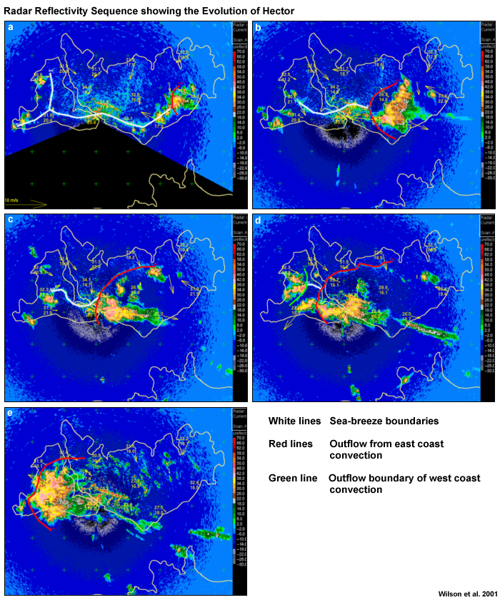
The key element of Hector is that it occurs on an island with little rugged topography, allowing the entire mesoscale convective system to propagate across the island. The site of initial convective initiation is determined by the low-level flow, and thereafter Hector propagates to the west.
What do you think happens in the case of islands with significant rugged topography?
(Type your answer in box.)
Feedback:
We will explore those situations in the following section.
Focus 1: The Australian-Indonesian Monsoon »
9F1.4 The Monsoon over the Maritime Continent »
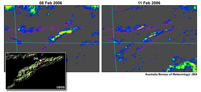
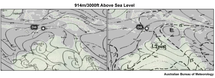
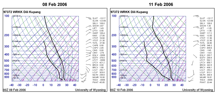
9F1.4.2 Timor and Convection over Significant Topography
Timor is an island with significant mountains. The highest point reaches 2963 m (9721 ft). Figure 9F1.23 shows the situation for two days in February 2006 with similar gradient level wind flow (3000’ above sea level). However differences in the wind profiles give rise to differences in convective cloud initiation and evolution (compare the left and right panels of Fig. 9F1.23). On the 8th the flow is east to northeast whereas on the 10th (11th was unavailable) flow is weak for much of the depth of the troposphere. On the 8th, the convection appears to form further inland along the spine of the island and is steered along the ranges. Later on the 8th, shallower convection in the Timor Sea is steered towards the northeast by the lower tropospheric flow. The slightly weaker near surface flow on the 11th allows convection to be generated near the coast, and on the ranges to the West of Dili. The steering flow then carries this convection into the Savu Sea.
What impact will these different situations have on forecasting for Dili airport? Review Fig. 9F1.23 before making your forecast.
(Type your answer in box.)
Feedback:
An expert response:
TAF WPDL 080105Z 0801/0814 31008KT 9999 BKN025
FM0813 14003KT 9999 SCT020
PROB30 INTER 0805/0810 5000 SHRA BKN010
TAF WPDL 110107Z 1101/1114 29011KT 9999 SCT025
PROB30 TEMPO1105/1111 1000 TSRA BKN010 SCT020CB
A chance of thunderstorms and rain (30% probability) at Dili was forecast on the 11th as the steering flow was easterly, possibly advecting the storms off the ranges and over Dili. On the 8th the steering was along the ranges so only showers and fewer clouds were forecast at Dili.
Focus 1: The Australian-Indonesian Monsoon »
9F1.4 The Monsoon over the Maritime Continent »
9F1.4.3 Papua New Guinea
Papua New Guinea’s (PNG) climate may not be described as truly monsoonal as there are no reliable periods of nil or near nil monthly rainfall as there is in Darwin, for example. Rainfall on the highlands is in the range 2500-3500 mm, with somewhat lesser values in the lowland areas. For example, Port Moresby has less than 1000 mm per year. Despite being tropical, frosts can occur above 2200 m and snow settles above 4000 m.
PNG rainfall is enhanced over the tropical oceanic regions due to two factors:
- the mountains of the Maritime Continent
- the West Pacific warm pool
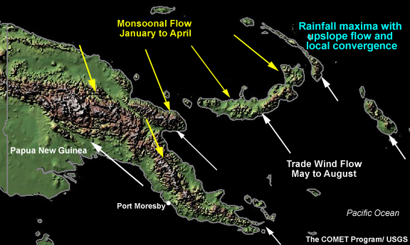
Both contribute to the maintenance of high θe air in this area. From routine satellite imagery, it can be seen that, cloud associated with the ITCZ affects PNG all year. However, the associated wind circulation patterns and the nature of the weather disturbances vary seasonally (Fig. 9.24).
During the southeasterly trades, convergence occurs where flow is onshore and undergoing frictional convergence and collision with nighttime land breezes (Fig. 9F1.24). During the monsoon, these convergences occur in different locations (Fig. 9F1.24). Throughout the year, enhanced uplift due to local topography leads to convection.146 Mountain-valley circulations also contribute to local convergence and convection.
Focus 1: The Australian-Indonesian Monsoon »
9F1.4 The Monsoon over the Maritime Continent »
9F1.4.4 The Indonesian-Malaysian Region
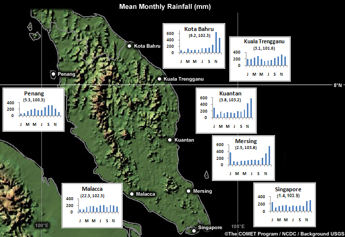
As was the case for PNG, enhanced topography can play a key role in the seasonal variation of rainfall throughout the Maritime Continent.147 Close to the equator there is a much less marked difference between wet and dry seasons than for the NAM. For example, Singapore has a relatively flat rainfall distribution (Fig. 9F1.25). The local rainfall minima occur in July and February under the influence of dry trade wind flows. The further north along the east coast, the greater the topographical enhancement of rainfall during the Boreal Winter (northeast) Monsoon. For example, the November rainfall at Kota Bahru is twice that of Singapore. Likewise, on the northwest coast a secondary peak exists in rainfall during April-May due to the southwesterly cross equatorial flow and the elevated topography.
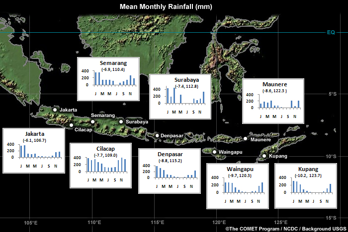
Java has a distinct dry season (Fig. 9F1.26), particularly in the south when under influence of southeast trade winds in the southern hemisphere (May to September). Likewise, there is a distinct wet season when influenced by Boreal Winter Monsoon (northeast trade winds). Sumatra (Fig. 9F1.27) also has a dry season under the influence of the southern hemisphere trades (May to September). The wet season is bimodal where mountains are able to enhance the northeast and southwest flows during boreal winter and summer respectively.

Intraseasonal variability
As with northern Australia, the MJO and various tropical wave modes such as the Kelvin wave, n=1 equatorial Rossby wave and mixed Rossby-gravity wave are responsible for intraseasonal variability over the Maritime Continent (Chapter 4, Section 4.1Chapter 4, Section 4.1) and references therein). Real-time monitoring of the MJO (Table 4.1)Real-time monitoring of the MJO (Table 4.1) and various tropical wave modes (Table 4.2various tropical wave modes (Table 4.2) is done routinely by NOAA and the Australian BoM.
However, as illustrated earlier in this section, knowledge of local topography is essential for forecasting rainfall over the Maritime Continent. For example, Haylock and McBride (2001)148 showed that the coherence of rainfall anomalies during December to February for two rainfall stations on Java separated by less than 100 km was small (correlation of 0.18).
NOAA/ESRL/PSD, OLR Modes, http://www.esrl.noaa.gov/psd/map/clim/olr_modes/
Focus 1: The Australian-Indonesian Monsoon »
9F1.5 Summary of the North Australian Monsoon
The differences between active, break and suppressed monsoon regimes for the North Australian Monsoon (NAM) are summarized in Fig. 9F1.28. The NAM is a result of the annual land-sea thermal contrast that develops during Austral Spring superimposed on the seasonal migration of the Hadley cell. The NAM is modulated by the Madden Julian Oscillation, upper troughs and equatorial waves, as well as by an inherent transient component of monsoon systems.125 Deep lows that move inland over Australia can produce dry southwesterly winds known as a suppressed or inactive monsoon. Significant enhanced topography over the Maritime Continent modifies the large scale synoptic flow such that knowledge of local topography is necessary to determine the seasonality and intraseasonality of deep convection.

Figure 9F1.28 shows a summary of the major features of the NAM. Like the Indian monsoon, the NAM undergoes alternating active and break monsoon periods with the migrating monsoon trough. The location of the trough exhibits an inherent transient nature but is also modulated by the MJO and equatorially trapped waves such as Rossby waves.
During the active monsoon, there is large scale forcing due to the monsoon trough, advecting a deep westerly, moist maritime air mass. Widespread cloud and precipitation occurs with relatively weak convective updrafts. The diurnal cycle is weak, with an overnight and morning maximum in convective activity due to its maritime nature but also an afternoon maximum over land due to boundary layer heating. Weather hazards, apart from tropical cyclones, include monsoonal squalls and flooding due to widespread, persistent rainfall from MCSs.
During break monsoon periods, widespread subsidence means that convection is forced locally on sea-breeze boundaries and is largely diurnal in nature. Short wave heating of the surface and long wave cooling of the mid troposphere contrast to the cold pool driven cooling of the surface and latent heating of the mid troposphere during the active monsoon. The result is isolated but more intense deep convection during the break period in the form of pulse convection, and various propagating lines of convection such as continental squall lines and Hector.
A third regime of the monsoon occurs when the monsoon trough is found in central Australia. Under these conditions, dry air wraps around a deep low, sometimes in the form of a “landfoon”, resulting in dry westerly winds over northern Australia and convectively suppressed conditions.
Focus 2: The Tropical Forecasters' Perspective
In order to understand how a tropical cyclone forecast is created, we interviewed two forecasters from NOAA's NHC (RSMC with responsibilities for the North Atlantic and Eastern Pacific) and one forecaster from Météo-France La Réunion (RSMC with responsibility for the South Indian Ocean). They also tell us about the path they took to tropical cyclone forecasting and changes in the forecast process during their careers.
Focus 2: The Tropical Forecasters' Perspective »
9F2.1 National Hurricane Center Forecasters (Audio Interviews)
Audio interviews were conducted with the NHC forecasters, Dr. James Franklin and Dr. Lixion Avila, on 9 June 2009. Here are edited versions of those interviews.
Dr. James Franklin
Question 1
How and when did you decide to become a tropical cyclone forecaster? What was your path? Did you do anything special in elementary or high school to further your goals?
Answer:
The path really began as a 6 year-old experiencing Hurricane Cleo when it went over my house, … but that's really what triggered my interest.
I didn't start out in forecasting at all. I was a researcher for 17 years, flying into storms with the hurricane research division of NOAA; did some operationally related research towards the end of that period when the GPS dropwindsonde got developed and spent some time looking at how hurricane winds behaved, the structure of those winds with height in the eye wall. That work caught the attention of some of the folks at the National Hurricane Center and they actually approached me about whether I had some interest in doing it. I hadn't really thought about it at all until they talked to me about it.
A lot of things in life I think are fortuitous. Being exposed to some hurricanes growing up; while I was in school at MIT, Bob Burpee who was at the Hurricane Research Division, was on sabbatical. I took his course on tropical meteorology, I guess I did well enough to have him approach me about a position.
All through high school, I had two main interests: one was meteorology the other was astronomy. Meteorology seemed to be the more interesting field, at least had more of an influence on people's lives and was a little bit more exciting. So that was the field I ended up taking. But I knew that going into college, that that's the kind of thing that I wanted to do, weather in general, I didn't know it was going to be hurricanes at the time.
I did spend a fair amount of my undergraduate time at MIT taking meteorology with folks like Fred Sanders, Pauline Austin, and spent some time with Fred, Kerry Emanuel going back and forth across the New England coastal front in Fred's Rabbit. My master's thesis was going to be on the New England coastal front. My good friend, Frank Marks, who was at MIT at the time, agreed to look over the collection of the data, while we went out and took the observations. Came back and found out the Frank had erased all the data instead of saving it and I was left with no thesis. Bob Burpee took me at the Hurricane Research Division anyway. A couple of years later, we came up with another thesis topic.
Question 2
What process do you use to forecast TC? What tools? Does your answer differ between track, intensity, size and rainfall forecasts?
Answer:
Track
Many years ago people could outfox the guidance at least in terms of track forecasting, but the numerical models have gotten so much better over the last 15, 20 years, in fact, our track forecasts are now about twice as good as they were 15 years ago. It's really very difficult for a forecaster to out integrate numerical models.
A very powerful technique in all of meteorology not just hurricanes is the idea of consensus. Get 3 or 4 or some group of skillful numerical models and you combine them. That's our goal; every time we sit down to make a forecast, that there is something that we can add to try and improve on that consensus. Is there a model that isn't initialized well? Do we recognize a situation when a certain model tends to perform well or tend to perform less well in? Very often your expectations for intensity play into the track forecast, but it all centers around the notion of a consensus and then trying to make moves in one direction or another from that.
One aspect of the forecast process has to do with presenting a consistent picture to our users. We have a very strong continuity constraint from one forecast to the next. We tend to make small increments on the forecast that came before us, improve what you inherited. I haven't talked about intensity so let me go on to that a little bit.
Intensity
Intensity forecasting is a little bit different then the track forecasting in the sense that guidance is not nearly so advanced. The forecast on the other hand does a better job than our intensity guidance. We have 4 intensity guidance models, 2 are dynamical, and 2 are statistical. The human forecaster can see a lot more of what's going on with the storm in terms of its convective structure and how the wind field is organized in terms of concentric eyewalls. None of the kinds of core factors is really well incorporated into our existing intensity guidance. By seeing what's going on in the core, that's where it is the forecaster really adds value to the guidance and is able to contribute a lot more to the process.
Size
We also forecast the size of tropical cyclones to issue these wind radii forecasts, the maximum extent of hurricane force winds in each of 4 quadrants around the center. So we are actually ahead of ourselves there in terms of what we provide relative to what we can do skillfully. So our error in even estimating that parameter is on the order of 50%. That a really tough one. About all that we have to help us with those are climatology and persistence models, the CLIPER model for example for wind radii. We have presumption that as a storm strengthens generally is it going to larger. After a storm is complete, we do what's called a best track, a post analysis of all the available data to create a permanent record, our best record of what happened with that particular storm: location, pressure, maximum sustained wind speed and the status, whether it's a tropical, subtropical, extra tropical. Until very recently we did not do a best track on the wind radius. Until you get to 2004, 2005, those are all operational estimates. They were not reviewed after the fact, those data certainly are not the same quality as the final best track intensity estimates. We've also got very few, sometimes no, real measurements of how large these radii really ought to be. From looking at the cloud shields, surface observations (these are very few), we have some additional tools to help us there. The AMSU, microwave instrument also gives us some size estimates.
Rainfall
Responsibility for rainfall forecasts lies with the Hydrometeorological Prediction Center. They are looking at model guidance, analogs, and previous storms. In our advisories now, we get the guidance for rainfall from HPC.
Question 3
Have ensemble model predictions changed your process?
Answer:
Ensembles are a big part of the tropical cyclone forecast process. Two primary methods would be to take a single model and run it repeatedly using slightly different initial conditions. That's one way. That has not been very successful in operational tropical cyclone forecasts. You can also form a consensus from different models.
When the members that make up an ensemble are independent you get a much better ensemble mean. We're also finding for intensity forecasting, if you form a consensus of the four main intensity models, it is much better on average than any of those four models individually. I think part of the reason for that is those models are very independent. They're not even the same type, you have two statistical models and you have two dynamical models and they're quite independent and it's that independence that really helps you. When members of an ensemble are independent, the errors tend to cancel, particularly when the synoptic situation is relatively simple, so we see this a lot in the eastern Pacific when the synoptic flows are simple. A lot of the errors in the models are random so if you can combine 3 or 4 of them you get a much better forecast then any individual one.
In the Atlantic the signal is not so strong. In the Atlantic we have stronger synoptic scale forcing, more complicated environments, midlatitude troughs coming down and a lot of other features in the environment and in that situation the different models are handling these features in different ways. The consensus concept in the Atlantic is a little bit less effective than it is in the east Pacific because there is more of a systematic component to how the models behave.
Question 4
What's your day like when there is a TC to forecast? How is it different if there are a number of TC? Is it any different if the TC are in different basins or in the same basin?
Answer:
Forecasting shifts are divided in to three: day, evening and midnight shifts. The day shift is responsible for 2 forecasts at 11:00 AM and 5:00 PM. The evening shift is responsible for the 11 PM advisory. The midnight shift is responsible for the 5:00 AM advisory. The day shift is longer, more tiring, much more hectic with more people floating around and more of a media presence.
The forecast cycle basically runs for 3 hours. The 11:00 AM advisory, for example, starts at 8:00 AM with an aircraft reconnaissance fix. You spend about 15 minutes analyzing the data from the reconnaissance aircraft, initial location, initial intensity, initial motion, initial size, all the parameters that are going to go into initializing the numerical model guidance. You update the best track and then submit guidance. We get it back and from about 8:30 AM and in this case up until 10:00 AM is spent making the forecast, looking at the models, the guidance, water vapor imagery, sea surface temperature all the different parameters that are important to track and intensity. By 10:00 AM you have your forecast prepared and we do a conference call with other weather service forecast offices as well as other agencies in the federal government. HPC will be on there, to talk about rainfall; the Storm Prediction Center will be on there, to talk about tornado threats; the Navy is there; Homeland Security is there; a whole host of agencies are there where we discuss the forecast, coordinate any issues that need to be coordinated, like where watches and warnings might be. That call can last from 3 or 4 minutes to a half an hour.
After the conference call is done we then prepare the forecast. We write our discussions and a summary of our rational behind the forecast. We talk about things like forecast uncertainty, why we've analyzed it to be the intensity that we have, why we've chosen the forecast that we have. That's a very important product for us used by emergency managers, the general public helps to provide some context for the forecast. In that last 45 minutes we're writing the discussion, we're preparing the public advisory.
If there are multiple storms you may have to do that for two and on occasion I've had to write even three advisories at once in that three hour period. We do have 2 forecasters on shift, but sometimes we may be working as many as 5 storms simultaneously between the Atlantic and east Pacific. There are times where you really have to compress it. It really depends on what kind of storms you have to deal with. If we have a significant landfall going on or imminent, within a couple of days of landfall, one of the forecasters will focus on that storm exclusively and leave 2 or even 3 to the other person if they are a less difficult forecast situation. We will try, when we have more than 3 systems, to bring in somebody to help us out. They are called hurricane support meteorologists; they have some experience in putting together advisory packages. They come in and help us with the least complicated of the systems that we're working on so that folks from the marine tropical forecasting unit, they're the folks that do the marine forecasting, or they might be from the technical support branch here at the hurricane center. They do have meteorology degrees, so some of them do have experience writing advisory packages. They're all Hurricane Center employees.
Dr. Lixion Avila (English)
Question 1
How and when did you decide to become a tropical cyclone forecaster? What was your path? Did you do anything special in elementary or high school to further your goals?
Answer:
I wanted to be a hurricane forecaster since I was a kid in Cuba and I was always asking questions to the farmers and to the fishermen. But, actually, I didn't start doing that until I was able to finish what you call pre-university degree in Cuba. I entered the Met Service in Cuba but I always wanted to be a hurricane forecaster. After that I went to the United States and I got my Masters and Ph.D. and I was lucky enough to enter the National Hurricane Center and I've been a forecaster for almost 25 years.
I got my degree in Cuba and I worked as a forecaster. But you take care of all the weather systems including hurricanes and I did that for about 5 years.
What I didn't know when I was in elementary school is that you needed a lot of math and physics to study meteorology but actually I love math and physics so it turned out to be good. That's one of the things that really got me by surprise. When you're a kid you don't know that you need those tools, you thought it was more like a fun thing to do than really study hard.
When I was a little kid, one of the things that I enjoyed was to wait for the afternoon thunderstorms, especially in the hurricane season. I grew up near the beach so there was some hills in between the ocean and the beach. Sometimes, I see the thunderstorms coming from south and sometimes I see the storms coming from the ocean. And it was really wonderful for me to enjoy the development of the clouds. And it was really interesting to see that. I am glad that my parents put up with that and they always pleased me with that craziness. But it turned out to be the best for me in the world.
Question 2
What process do you use to forecast TC? What tools? Does your answer differ between track, intensity, size and rainfall forecasts?
Answer:
I've been doing this since 1971. I have seen how the tools have changed. Tremendously! In the '70s we were plotting the surface data by hand. We were getting, maybe, one map a day of a forecast of 24 hours at 500 mb. The facsimile; we even got 1 satellite picture or two satellite pictures a day. And that was probably the case in most of the Caribbean countries and probably not very different in the United States.
We began to get more and more satellite pictures…What really changed the way of forecasting is the development of numerical models and computer science. And, nowadays, we can use all these sophisticated computer models and the physics and dynamics that goes into models to predict hurricanes.
First thing we do in the morning, is to look at the entire globe and all the satellite pictures and look at the different systems. Then we emphasize the system that we think is going to do something or not. We look at the analysis of what's going on through the computer models, of course, using the, also, the conventional data. Before I wasn't able to integrate in my head 5 days in advance, now the computer models are able to give me a better estimate, at least, what could happen, or the possibilities that could happen in terms of the distribution of high pressures and low pressures.
Nowadays we make a 5-day forecast and the weather pattern that is going to affect that cyclone today, if it's in the Caribbean, that weather system is, perhaps, in the western Pacific now, then move to the east. So we need to look at the whole pattern. Either track or intensity, you have to look at the whole thing because the intensity change is related to, perhaps, an upper trough coming. It is more difficult, of course, the forecast of the intensity.
Size
At this moment when we make a prediction, if we don't have data, we don't even know the size of the system. So what we do is try to extrapolate. But we don't have any tools to predict changes in size other than climatology. Perhaps some of the numerical models would give us the size of the storm when they are moving and becoming extratropical in higher latitude. The models are doing a little better, but in terms of the deep tropics the change and size, it's very difficult to predict. What we do is just basically use extrapolation and when we get new data that tell us that the size is larger, we adjust with the new data.
Rainfall
In terms of rainfall, it's even more difficult. Rainfall is probably the cause of most of the deaths, for example, in the region of the Caribbean. But it's the same in most of the tropics when you even have a small, weak tropical depression that could produce 20 inches of rain and produce a tremendous amount of damage. And, unfortunately, many people are killed by the rainfall, especially by flash floods and all this orographic rain that you have when you have a weak tropical depression. Those are very difficult, difficult processes, both the size and the rainfall.
You know, the intensity of a tropical cyclone has nothing to do with the rainfall. It's basically the speed and the amount of convection that the system has. You can have a hurricane that can produce less rain then a weak tropical depression.
There are some old rules I learned from the old-timers and they use the number 100 divided by the speed of the tropical cyclone and you get the amount of inches of rain. And it's so interesting to see that some models, like the GFDL and others, when you compare with that rule the numbers on average turn out to be very close. The bottom line is that it's the speed of the system what matters.
Question 3
Have ensemble model predictions changed your process?
Answer:
Here at the National Hurricane Center, what we have been using is another type of ensemble. What we call the "consensus", which is not just the ensemble of one model but the consensus of different models. And, actually, that turns out to be one of the best ways of making a forecast. It appears that, when you make the consensus of different models, you cancel all the biases of the models and you end up having a better forecast by using all these consensus models.
Yes, it changed the process and makes my life, I would say, a little bit easier. But, still, you have to understand why each particular model is doing what it's doing. You cannot use models as a black box, you have to understand what goes into each model.
In many cases here, when we do the verification, the forecaster turns out to be better than all the different independent models. Because we are using all the information and we process it and we get, as I mentioned, we understand the strength and weakness of each model and we try to improve on that.
Question 4
What's your day like when there is a TC to forecast? How is it different if there are a number of TC? Is it any different if the TC are in different basins or in the same basin?
Answer:
Things have changed too, throughout the years. I do remember when we were 5 hurricane specialists and I have to do almost all of them. And now, luckily, we have more specialists and we get help from other colleagues here at the National Hurricane Center. We are prepared to have simultaneous tropical cyclones. Of course, the pressure is tremendous, especially if you have a hurricane that is threatening land areas. If it's a strong hurricane, we have to take care of the media. But, our emphasis is to be able to get all the information and try to make the best forecast possible.
Do I get nervous? No. Do I get excited? Yes! I do get very excited. I have to be in control, but always, what I like to do is emphasize on the science. I don't want to be biased by any of my feelings and I want to do the best job possible. But, it's a very interesting day. It's a very interesting day when you have a tropical cyclone. I presume that it is the same with a doctor when they have somebody that they want to cure or they want to improve their health. I want to make the best forecast.
I've been offered to work for insurance companies. I have been offered to work for TV. But, there is something about being here at the National Hurricane Center; that I have the "power" to name a system. You might think it's not important, but for me, it kind of means that I'm on top of the science and I'm doing this. For me, it's one of the fun things that I get from the job.
| Dr. James Franklin | Question 1How and when did you decide to become a tropical cyclone forecaster? What was your path? Did you do anything special in elementary or high school to further your goals? Click Question 2What process do you use to forecast TC? What tools? Does your answer differ between track, intensity, size and rainfall forecasts? Click Question 3Have ensemble model predictions changed your process? Click Question 4What's your day like when there is a TC to forecast? How is it different if there are a number of TC? Is it any different if the TC are in different basins or in the same basin? Click |
Dr. Lixion Avila (English) Click to view these interviews in Spanish. | Question 1How and when did you decide to become a tropical cyclone forecaster? What was your path? Did you do anything special in elementary or high school to further your goals? Click Question 2What process do you use to forecast TC? What tools? Does your answer differ between track, intensity, size and rainfall forecasts? Click Question 3Have ensemble model predictions changed your process? Click Question 4What's your day like when there is a TC to forecast? How is it different if there are a number of TC? Is it any different if the TC are in different basins or in the same basin? Click |
Focus 2: The Tropical Forecasters' Perspective »
9F2.2 Tropical Cyclone Centre Météo-France, La Réunion
Interview with Dr. Anne-Claire Fontan, tropical cyclone forecaster
1. How and when did you decide to become a tropical cyclone forecaster? What was your path? Did you do anything special in elementary or high school to further your goals?
I became a tropical cyclone forecaster at the RSMC/Tropical Cyclone Centre Météo-France/La Réunion 12 years ago, once I finished studying at the French school dedicated to meteorology “ENM” (Ecole Nationale de la Météorologie de Météo-France / Météo-France National School of Meteorology), located in Toulouse, France. This school gives a diploma in meteorology, which takes three years to complete (after either two years in a university-level college, or a Master of Science at the university).
Before this school, I was at university where I studied for a Masters degree in oceanography and meteorology at Marseille and Paris. In France, there is no way to specialize in meteorology until you have completed a bachelor or Masters degree or the “ENM”, but you need to choose a scientific path from high school.
Once you have graduated, and got the job at the RSMC/TCC La Réunion, you have to follow an extra two weeks formation in tropical meteorology. Afterwards you become a “trainee” in operations during several months at the RSMC. During this period you are given an additional formation and practice through tutoring with experienced TC forecasters. A TC forecaster is considered to be accomplished after one or two complete cyclonic seasons.
2. What process do you use to forecast TC? What tools? Does your answer differ between track, intensity, size and rainfall forecasts?
To forecast at the RSMC/La Réunion, we use a powerful workstation called SYNERGIE. This workstation displays and superimposes all the data a forecaster needs to work: observations, models, satellite imageries, radar, etc. There is a specific module dedicated to tropical cyclones called SYNERGIE CYCLONE which allows us to focus on tropical cyclone analysis and track and intensity forecasts. In addition to models, observations, images, and TC tracks plots, we have recently implemented the possibility to display directly the websites data we use daily in operation. These websites are mainly – and so not exhaustively - the tropical cyclones pages from the NRL, the CIMSS, the NOAA (QuikSCAT), the AOML (heat potential), the Australian BoM (MJO), ….
Our area of responsibility (Equator to 40°S and African coastline to 90°E) is mainly a maritime basin, except the western part between African coasts and 60°E. We rely indeed a lot on satellite data. Size and rainfall associated to the systems are “observed”, not yet specifically forecast. Every 6 hours, as we issue our warnings, we describe the size of the TC, based on the 30 knots and 50 knots winds, by using all the available observations; these are mainly received through scatterometer data - due to the maritime characteristic of our basin. We also describe the weather and the rainfall associated with the system. When a TC is forecast to approach or hit a landmass the “comments part” of the warnings specifies as well the inhabited areas the rainfall can concern in the next 24 to 36 hours. In this case, we use forecast fields as the precipitation rate, humidity, vertical velocity, …, of the best model.
Track forecast
We get the fields from the numerical models developed by different countries/centres to be able to track forecast; two models from Météo-France, a global one and a limited area one (over Southern Indian Ocean), one from the UKMO (United Kingdom Met Office), and the Ensemble Prediction System (EPS) average and the deterministic models from the ECMWF (European Centre). Since season 2004-2005 we get as well the “geopoints” (i.e. position and MSLP (Mean Seal Level Pressure) of the TC each 6 or 12 hours) of some of the American numerical models via the JTWC; GFDN, NOGAPS, AVNO, and consensus of different models computed at the JTWC. These models tracks are displayed on the workstation.
Thanks to the analysis of the fields from the models, the forecaster decides which scenario is the best. Afterwards, as statistics tend to show consensus of models lead to the better results, we average chosen models to make the track forecast. If philosophy of some of the models totally differs from the chosen one, we do not involve them in the average.
Intensity forecast
To forecast intensity, we need to know the current and follow-on environment of the system. Several tools are used. We study the products of the CIMSS to get the current environment and to get it for the few hours to come; upper level divergence and winds, low level convergence and winds, wind shear, shear tendency, and so on. We get the heat content thanks to the SSTs satellite data and the AOML website heat potential (depth of the 26°C isotherm). Humidity is assessed thanks to WV and MW imageries. Then we use the fields of the model estimated to be the best for the situation: θ’w at 700 hPa, divergence, convergence. And we have a look on the tendency of the different models, if ever they deepen or weaken the system.
3. Have ensemble model predictions changed your process?
For the past few years we received data from the Ensemble Prediction System (EPS) and it has changed the way we work and our results. We use it to further several goals. First of all, the EPS is used to assess the probability of cyclogenesis over the basin for the 10 coming days. Then the average of the 51 runs of the EPS is used as a ”deterministic model” and can be involved into a consensus of models to make the TC track forecast. Strike probabilities provided on each system by the ECMWF is used to manage the risk at La Réunion Island. The last goal, still under investigation, would be to use the EPS to provide cones of uncertainty for the RSMC forecast track.
4. What’s your day like when there is a TC to forecast? How is it different if there are a number of TC? Is it any different if the TC are in different basins or in the same basin?
We work in 12 hour shifts either day or night. These shifts range between 7.00 AM to 7.00 PM and 7.00 PM to 7.00 AM. We issue four series of warnings a day at 00, 06, 12, 18Z. So for example, for a day shift we have the 06 and 12Z warnings to issue.
At first we have the changeover and a detailed study of the current situation. At 08.30 AM we have the briefing for the people working at the centre. Straight afterwards starts the entry of the data in the software we use to prepare the 6 or 7 warnings which will be issued in both English and French at 10.30 AM (0630Z). Then we brief the local weather forecast service and if necessary (i.e. if the TC directly or indirectly concerns the weather on Réunion Island), we provide it with guidance and directives. We have a break between 11.00 AM and 12.00 PM.
Afterwards, we have a database dedicated to cyclogenesis to fill in, and the writing of the tropical weather outlook in both English and French, which will be issued at 03.00 PM. Meanwhile we write the “connection bulletin” which allows to keep the information within the team, and to give instruction for the three following days to the local forecast team.
The following warnings are prepared and issued at 04.30 PM. At the end of the shift, we have to update the archives of the day with messages, pertinent satellite images, and so on.
When there is a risk to manage on Réunion Island, we issue some extra warnings at 1.00 PM and 7.00 PM for the local authorities and for the public, and we answer to the media.
If ever there are two TC to deal with, it is double the workload! If there are two systems to monitor, with a risk to manage on the Island, a second cyclone forecaster comes to help. We get somebody in extra as well if ever there are more than two systems over the basin.
We have a single basin to monitor. But this basin has a “virtual border” with two others ones; the south-east Indian Ocean (the Australian area of responsibility starts at 90E) and the Indonesian area of responsibility (east of 90E, north of 10S). If ever a TC comes from one of their areas of responsibility to ours or vice versa, the different centres (Perth, Jakarta and Réunion Island) send e-mails or phone to manage the handover.
Focus 2: The Tropical Forecasters' Perspective »
9F2.3 Météorologique Régional Spécialisé / Centre des Cyclones Tropicaux de La Réunion, Météo-France
Entretien avec Anne-Claire Fontan, ingénieur prévisionniste cyclone
1. Comment et quand avez-vous décidé de devenir un prévisionniste cyclone? Quel a été votre cursus? Avez-vous suivi un parcours spécifique que cela soit en primaire, collège ou lycée pour atteindre votre but?
Je suis devenue ingénieur prévisionniste cyclone au CMRS/ Centre des Cyclones Tropicaux de La Réunion il y a 12 ans, une fois mes études terminées à l’ENM (Ecole Nationale de la Météorologie), l’école d’ingénieurs dédiée à la météorologie, dépendant de Météo-France, et située à Toulouse, en France. Cette école délivre un diplôme en météorologie qui nécessite trois ans d’étude ( qui viennent après deux ans de classes préparatoires aux grandes écoles ou une maîtrise de sciences de l’université). Avant l’ENM, j’ai fait mes études dans les Universités de Marseille et Paris pour obtenir un Master d’océanographie et de météorologie. En France, il n’est pas possible de se spécialiser en météorologie avant l’université et le niveau licence ou maîtrise -ou avant d’aller à l’ENM, mais il est toutefois nécessaire de choisir une filière scientifique dès le lycée.
Une fois diplômé et une fois obtenu le poste au Centre des Cyclones Tropicaux de La Réunion, il faut suivre deux formations supplémentaires; une première formation théorique de deux semaines en météorologie tropicale à l’ENM, puis une deuxième formation, opérationnelle, pendant plusieurs mois, au Centre des Cyclones. Cette période consiste à travailler avec et sous la supervision d’ingénieurs prévisionnistes cyclone expérimentés. Un prévisionniste cyclone est dit confirmé après avoir travaillé pendant une ou deux saisons cycloniques complètes.
2. Quelle(s) méthode(s) utilisez-vous pour prévoir les cyclones tropicaux (CT)? Avec quels outils travaillez-vous? Si l'on distingue les prévisions à effectuer: trajectoire, intensité, taille ou précipitations, vos réponses sont-elles différentes?
Pour élaborer les prévisions au Centre des Cyclones de La Réunion, nous utilisons une puissante station de travail appelée SYNERGIE, sur laquelle nous pouvons visualiser et superposer toutes les données dont un prévisionniste a besoin pour travailler: observations, modèles, imageries satellite, radar, etc. Cette station de travail possède un module spécifiquement dédié aux cyclones tropicaux (SYNERGIE CYCLONE), avec lequel nous travaillons pour procéder à l’analyse du système tropical et établir les prévisions de trajectoire et d’intensité. En plus des modèles, observations, images et tracé des trajectoires issues des modèles numériques …, nous avons récemment installé la visualisation directe des données des sites Internet utilisés quotidiennement en opération. Ces sites sont principalement – et donc de manière non exhaustive- les pages dédiées aux cyclones tropicaux du NRL, du CIMSS, de la NOAA (QuikSCAT), de l’AOML (pour le contenu énergétique), du BoM australien (MJO), ….
Notre zone de responsabilité (de l’équateur à 40S et des côtes africaines à 90E) est essentiellement un domaine maritime, exceptée la partie ouest du bassin, entre les côtes africaines et le 60E. Nous dépendons donc fortement des données satellitaires.
La taille et les précipitations associées aux systèmes tropicaux sont « observées », mais ne sont pas encore spécifiquement prévues. Toutes les six heures, lors de la diffusion de nos bulletins, nous décrivons la taille des systèmes via l’extension des vents à 30 nœuds et 50 nœuds, essentiellement grâce aux données des diffusiomètres (du fait du caractère maritime du bassin). Nous décrivons également le temps et donc les précipitations associées au système. Lorsqu’un système tropical est prévu approcher ou frapper une terre, la partie « commentaires » de nos bulletins spécifie de plus les zones habitées que les précipitations peuvent concerner dans les 24 à 36 prochaines heures. Pour ce faire, nous utilisons les champs prévus comme le taux de précipitation, l’humidité, la vitesse verticale, …, du meilleur modèle.
Prévision de trajectoire:
Pour élaborer nos prévisions de trajectoire, nous disposons des champs des modèles numériques développés par différents pays ou centres; deux modèles de Météo-France, un global et un à aire limitée sur l’Océan Indien Sud, le modèle anglais du Met Office, le modèle déterministe et la moyenne de la prévision d’ensemble du Centre Européen de Prévision (CEP). Depuis la saison 2004-2005, via le JTWC, nous avons également accès aux « géopoints » (i.e. position et pression minimale au centre du système tropical, toutes les 6 ou 12 heures) de quelques-uns des modèles américains comme le GFDN, le NOGAPS, le AVNO, et consensus de modèles calculés au JTWC. Les trajectoires proposées par tous ces modèles sont visualisées sur la station de travail.
Grâce à l’analyse des champs des modèles, le prévisionniste décide quel scénario est le meilleur. Par la suite, comme les statistiques tendent à montrer que les consensus de modèles mènent aux meilleurs résultats, nous moyennons les modèles choisis pour élaborer la prévision de trajectoire. Si la philosophie de certains modèles ne correspond pas à celle retenue, nous ne les incluons pas dans la moyenne.
Prévision d’intensité:
La prévision d’intensité nécessite la connaissance de l’environnement du système et son évolution. Nous utilisons pour ce faire plusieurs outils. Nous étudions les produits du site du CIMSS pour connaître l’environnement; la divergence et les vents d’altitude, la convergence et les vents de basses couches, le cisaillement vertical de vent et sa tendance, etc. Nous regardons le potentiel énergétique océanique via les températures de surface de la mer données par l’imagerie satellite et le contenu énergétique du site de l’AOML (profondeur de l’isotherme 26°C). L’humidité est évaluée grâce aux imageries vapeur d’eau et micro-onde, et nous utilisons également les champs du modèle estimé être le meilleur; θ’w à 700 hPa, divergence, convergence. Pour finir, nous regardons la tendance donnée par les modèles, s’ils creusent ou affaiblissent le système tropical.
3. La Prévision d'Ensemble a-t-elle changé votre méthode de travail?
Nous somme destinataires des produits de la Prévision d’Ensemble (PE) depuis plusieurs années et cela a changé notre façon de travailler et nos résultats. Nous l’utilisons à différentes fins. Tout d‘abord, la PE est utilisée pour évaluer la probabilité de cyclogenèse à 10 jours sur le bassin. Ensuite, la moyenne des 51 runs de la PE est utilisée comme un modèle déterministe et peut être incluse dans un consensus de modèles pour élaborer la prévision de trajectoire. Le panache de probabilité (« strike probabilities ») fourni par le CEP sert à la gestion du risque sur l’Ile de La Réunion. Enfin, la dernière application, toujours à l’étude, serait d’utiliser la PE pour calculer des cônes d’incertitude appliqués à la prévision de trajectoire du CMRS.
4. Comment se déroule une journée de travail lorsqu’un système tropical évolue sur le bassin? En quoi est-ce différent s’il y a plusieurs systèmes tropicaux à la fois? Suivant si les systèmes tropicaux évoluent sur le même bassin ou bien sur des bassins différents, cela fait-il une différence dans votre journée de travail?
Nous travaillons selon des tours de service de 12 heures, qui peuvent être de jour ou de nuit. Les horaires de ces tours de service sont de 07h00 à 19h00 et de 19h00 à 07h00. Nous émettons quatre séries de bulletins par jour, en français et en anglais, à 00, 06, 12 et 18Z. Nous avons donc lors d’une journée de travail, les bulletins de 06 et 12Z à élaborer et diffuser.
La journée commence avec la relève et l’étude approfondie de la situation, exposée lors d’un briefing pour le personnel du centre à 08h30. Nous enchaînons avec la saisie de données dans le logiciel avec lequel nous préparons nos 6 à 7 bulletins, qui sont diffusés en bilingue pour 10h30. Vient ensuite le briefing interne avec le service de prévision du temps local et si nécessaire (i.e. si un CT concerne directement ou indirectement le temps sur La Réunion), nous lui fournissons des directives.
Nous avons une pause entre 11.00 AM et 12.00 PM.
Après cela, nous devons remplir une base de données concernant la cyclogenèse, et débuter la rédaction du bulletin en anglais et français sur l’activité cyclonique et les conditions météorologiques du bassin (« tropical outlook »). Ce bulletin est diffusé à 03h00. Entre-temps, nous élaborons le bulletin dit de « liaison » permettant de tenir l’équipe informée des actions de la journée et de donner des instructions à l’équipe de prévision locale pour les 3 jours à venir.
Les bulletins du réseau suivant sont ensuite préparés et diffusés pour 04h30. A la fin du service, nous procédons à l’archivage des messages, des images satellitaires pertinentes, etc, de la journée.
Si jamais nous avons deux CT à gérer, c’est double travail! S’il y a deux systèmes à suivre, avec une gestion de risque sur La Réunion, un deuxième prévisionniste cyclone vient donner de l’aide. Quelqu’un vient également en renfort lorsqu’il y a trois systèmes à gérer sur le bassin.
Nous avons un seul bassin à surveiller, mais il a une frontière « virtuelle » avec deux autres zones; le sud-est de l’océan Indien (la zone de responsabilité australienne débute à 90E) et la zone de responsabilité indonésienne (est de 90 E et nord de 10S). Si jamais un CT nous arrive d’une de ces deux zones (ou vice et versa), les centres concernés (Perth, Jakarta, La Réunion) s’envoient des mels ou s’appellent pour assurer la passation de responsabilité de suivi du système.
Summary
Tropical weather observation, analysis, and forecasting are challenging but continue to improve thanks to new instruments (mostly satellite and some in situ), derived variables, and tools for synthesizing observations and numerical model output. Forecasters add value to the automated systems using their knowledge of model biases, rapidly updated satellite information, and past cases. Satellite data analysis is one of the most critical skills for tropical weather forecasters. Since radars are sparse in the tropics, high resolution geostationary images aid in nowcasting mesoscale and convective-scale weather systems. High resolution, non-hydrostatic models are producing realistic convective weather systems at many scales, however, data assimilation methods are challenged by increasing amounts and types of satellite data. Ensemble techniques are providing information on model forecasts uncertainty. Multi-model ensemble (consensus) models have led to better tropical cyclone track forecasts. While tropical cyclone intensity forecast skill is lagging, ensembles of statistical and high-resolution dynamical models provide the best numerical guidance currently. Intraseasonal forecasting is becoming mature enough to be used as guidance for the probability of tropical cyclogenesis. New and traditional forecast verification and validation techniques are helping tropical forecaster evaluate numerical forecasts. As knowledge of tropical meteorology and confidence in NWP increases, we expect to see more improvements in tropical weather forecasting.
Appendix A: Station Plot and Weather Symbols
Surface station data are plotted at its location on a weather map in a format shown in Fig. 9A.1. To the upper right is mean sea-level pressure (MSLP); the leading digit(s) is dropped (9 or 10 in the case of MSLP). Therefore, a MSLP value of 998.6 hPa is plotted as “986” while 1011.5 is plotted as "115". The circle shows the sky cover in eighths or oktas (Fig. 9A.2). The wind barb represents speed and the direction from which the wind is blowing. For standard upper-air horizontal analyses (1000, 850, 700, 500, 300, 200 hPa), the station plots show temperature, dewpoint, wind velocity, and geopotential height. A sample 850 hPa data plot is shown in Fig. 9A.1b, where geopotential height of 1564m is plotted as “564”. Other commonly used weather symbols are shown in Fig. 9A.2.
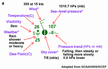
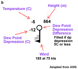
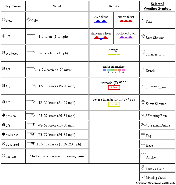
COMET module: Introduction to Meteorological Charting
NOAA/NWS, How to read surface weather maps,
http://www.srh.noaa.gov/jetstream//synoptic/wxmaps.htm
Questions for Review
- Describe at least two challenges that are unique to tropical weather forecasting.
- List three types of point measurements.
- List three sources of observation error.
- What are the advantages and weaknesses of satellite observations when compared to station observations of the tropics?
- Describe two advantages and two limitations of weather radar observations for tropical weather analysis and forecasting.
- Why is streamline/isotach analysis more useful for tropical weather forecasting than isobaric analysis?
- List at least two instruments (in situ or remote-sensing) developed for research that have been applied to tropical weather forecasting since the 1990s.
- How does monitoring intraseasonal circulations, such as equatorial waves and the MJO, help tropical forecasters?
- List uses and limitations of trajectory analysis for tropical weather forecasting.
- List three variables forecasted for tropical marine weather.
- Describe how satellite and radar images are used to analyze the evolution of tropical mesoscale convection.
- Describe at least four sources of numerical weather prediction model error.
- What is the purpose of data assimilation?
- What are the fundamental principles represented by the “primitive equations” used in dynamical models?
- Why are non-hydrostatic models better for tropical weather prediction than hydrostatic models?
- Explain what constitutes an ensemble numerical forecast.
- Describe the advantages and limitations of three-dimensional (3D-VAR), four-dimensional variational (4D-VAR), and Ensemble Kalman Filter data assimilation techniques.
- Describe three methods for verification of NWP model forecasts including their strengths, weaknesses, and at least one example of their application in tropical weather.
- List three factors that must be considered when forecasting tropical cyclone motion.
- List three factors that must be considered when forecasting tropical cyclone intensity change.
- When are statistical models most useful in tropical cyclone forecasting?
- What are some of the key physical variables included in a typical statistical model used for tropical cyclone forecasting?
- Give a basic description of two dynamical models used for tropical cyclone motion forecasts.
- When are ensemble techniques most useful for tropical cyclone prediction and why?
- Describe two techniques used to validate tropical cyclone motion or intensity forecasts.
- List the major differences between active and break monsoon periods over Northern Australia in terms of dynamics and thermodynamics.
- Describe the differences in the diurnal cycle of convection between active and break monsoon periods. What impact does this have on aviation forecasting at Darwin, Australia?
- List as many of the severe storm types you can and at least one feature in the radiosonde that would alert you to potential severity.
- Briefly describe why suppressed monsoon periods occur over northern Australia. How are these periods different to the typical active monsoon?
- What role does orography play in the seasonal cycle of precipitation over the Maritime Continent (SE Asia)?
QUIZ
You may also take a quiz and email your results to your instructor.
Brief Biographies
Dr. Akio Arakawa
Dr. Akio Arakawa is a pioneer in global numerical weather prediction (NWP). He received his B.Sc. in physics and D.Sc. in meteorology from Tokyo University in 1950 and 1961, respectively. While working at the Japan Meteorological Agency during the 1950s, he developed his first global atmospheric circulation model, having been inspired by Norman Phillips’s first general circulation simulation. He came to the University of California Los Angeles (UCLA) as a visiting scientist in 1961 after being recruited by Yale Mintz. In 1963 they completed the first UCLA General Circulation Model, which later became known as the Mintz-Arakawa Model. It was the first global model to include realistic land-sea distributions and surface topography. Arakawa returned to UCLA in 1965 after a two-year period in Japan. He remained at UCLA as a faculty member for the rest of his career while leading the development of increasingly sophisticated general circulation and earth system models.
Using his brilliant mathematical skills and meteorological expertise, he developed numerical methods for representing fluid dynamics including finite difference techniques first published in 1966. He also developed robust schemes for representing the interaction of cumulus convection and large-scale circulations, creating with Wayne Schubert, the “Arakawa-Schubert cumulus parameterization scheme” in 1974. These contributions have led to major advances in tropical weather prediction and earth system modeling in general. He received the Carl-Gustaf Rossby Research Medal in 1977, the highest award granted by the AMS. His career was celebrated at UCLA in 1998 with, “General Circulation Modeling Past Present, and Future: A symposium in honor of Akio Arakawa. He was made a Fellow of the AMS and an AMS symposium was held in his honor in 2007. He was a recipient of the UCLA Dickson Award for 2008. Most recently, he was awarded the 2010 Vilhelm Bjerknes Medal by the European Geosciences Union in recognition of his pioneering and fundamental contributions not only to numerical modeling in atmospheric sciences but to geophysical fluid dynamics in general. Although retired, he continues to be involved in ongoing efforts to refine global models including climate models. He is regarded as a “living legend”.
Benito Viñes (1837-1893)
Known as the “Hurricane Priest”, Father Benito Viñes, laid the foundation for the modern observational and hurricane warning network. He was the director of the Magnetic and Meteorological Observatory of the Royal College of Belen in Havana, Cuba from 1870 until his death in 1893. He was born in Poboleda, Spain, received training in physics, and came to Cuba via France. He organized hundreds of observers to monitor weather along the coast of Cuba, thereby establishing the first observational network that delivered hurricane warnings by pony express and later by telegraph. From his meticulous observations of surface weather, cloud motion, sea-swells, and post-landfall assessment, he developed a fairly accurate conceptual model for the three-dimensional structure of hurricanes. By observing cloud motion and sea swells, he also created a technique for finding the center of hurricanes. He became famous for pioneering forecasts of hurricane motion based on the movement of high cloud outflow from the center of tropical storms. In September 1875, he became a legend after he issued his first printed forecast and accurately forecasted the landfall of an intense hurricane in southern Cuba. Subsequent success later that year and in the following years resulted in Viñes gaining funding from private companies to aid with observation stations and free message service from telegraph and railroad companies. He published his now famous Practical Hints in Regard to West Indian Hurricanes in 1877 and it became a standard training resource for mariners and others. His technical report on the Cyclonic Circulation and Translatory Movement of West Indian Hurricanes was delivered posthumously to the U.S. Weather Bureau, having been mailed three days before his death.
Thanks to Patrick Fitzpatrick for sharing biographical information from his book, "Hurricanes; a reference handbook, 2nd Edition", Contemporary World Issues, ABC CLIO, 412pp, 2006.