
The constant gentle pitter-patter of short wavelength gravity waves in the real atmosphere can be reproduced in models with grid spacings of 1 or 2 km but becomes more like silence interrupted by a periodic "boom!" in models with resolutions typically used for NWP. The nature of the adjustment process in response to imbalances in initial conditions and imbalances created by forcing from latent heating and forcing from other model physics is often impulsive. Thus, model behavior corresponds more closely to the theory described on the first few pages here than to the smoother adjustment process typical in the real atmosphere.
What do we mean by "balanced" mass and winds?
Model fields are "balanced" when the dynamics and physics in the model are consistent.
Divergence and vertical motion are consistent with forcing caused by surface
friction, latent heating, flow over orography, frontal upglide, jet streak
dynamics, etc.
Changes in divergence and vertical motion following a weather feature tend
to be gradual
Conditions may
Start out unbalanced because the analysis may not be entirely consistent
with the model topography, physics, resolution, or other aspects of the
model
Become unbalanced during the forecast due to sudden bursts of latent heating by convection, by fast flow over topography, or any other quickly-imposed strong forcing
When the model has unbalanced conditions, it emits gravity waves and adjusts
toward a balanced state. The intensity, scale, and duration of the impact on
the forecast depends on the magnitude of the imbalance and whether it is dynamically
large or small (remember, its wavelength, L, compared to 2 LR).
LR).
How initial imbalance affects the forecast
Unbalanced initial conditions cause gravity wave noise early in the forecast. The adjustment process may also change the large-scale features somewhat. Here is an example from the 22-km operational Eta model and the nested 10-km Eta regional run.
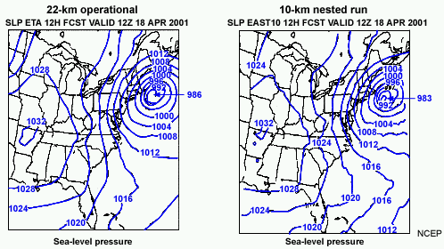
The 22-km Eta fields are smooth. The 10-km Eta isobars are wiggly pretty much all over, with even some isolated spots of 1032mb over central AR and northern LA.
The wiggles are characteristic of running a model without balanced initial conditions
The wiggles in this case may also be partly due to latent heating in the model cyclone (discussed in the next section below)
3D-VAR and assimilation cycling combine to make smooth, "balanced" initial conditions for the 22-km Eta model
The wiggly behavior typically results from using model initial conditions purely from data or from a different model or from the same model at different resolution, because of the inconsistencies introduced
Initialization procedures modifying model analysis fields are used to minimize this problem when the analysis procedure does not generally yield sufficiently balanced initial conditions
The 10-km Eta initial conditions were interpolated from the 22-km Eta,
and a digital filter was applied to eliminate small-scale noise. Testing
in other cases without using the filter showed considerably worse problems
Also, notice the larger-scale modifications away from the cyclone: the shift of the 1028hPa contour over southwest WI, the 1024 hPa contour over eastern MI and northern FL, the 1016hPa contour over eastern NC and VA, and the strength of ridging over the water off the southeast coast. Resolution is probably not the primary cause of these differences.
Initial condition differences due to the digital filter may have resulted in these forecast differences at 12 hours
Adjustment due to initial imbalances may have caused the model to move
toward a different large-scale state. Not only is gravity-wave noise generated,
but also the large-scale balanced fields can be modified. Experiments in
other cases without the digital filter found even bigger large-scale adjustments
How imbalance generated by physics forcing affects the model forecast
The model responds to intense sudden changes by sending out gravity waves and beginning the adjustment process to bring those changes into "balance." A dramatic example caused by intense latent heating from the grid-scale precipitation parameterization is shown here.
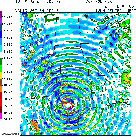
|
This 12-hour forecast plot from a hydrostatic 10-km Eta threats run shows 500hPa vertical velocity in microbars per second, negative for upward motion. The white area in the center of the ring pattern is rising at more than 40 microbars/second. Instead of the grid-scale precipitation scheme steadily releasing latent heat over the eight minutes between the times it updated, this older version of the model was releasing all that latent heating in 24-second bursts. The model responded to the sudden changes with gravity waves. Cloud models (such as with grid spacing of 1 km or smaller) respond to the initiation and collapse of vigorous updrafts with a display of outward-propagating gravity waves, and satellite pictures of convection sometimes reveal waves in nature as well, though in both a cloud model and nature, the wavelength and area affected are smaller than in the example shown here. |
As a forecaster, you need to note several things:
The gravity wave noise masks the mean signal. This is not only true of the model: raw (not time-averaged) wind profiler observations tend to be dominated by short-period vertical motion oscillations that mask the weaker large-scale signal
The gravity waves may modulate other features in the model, causing them to appear to line up with the waves
The most important forecast impact is what happens to the feature once
its forcing ends. In this case, what will happen over 12 hours, 24 hours,
even 72 hours, to the vorticity and height perturbations associated with
this precipitation bull's-eye over south-central Texas once the precipitation
weakens? The answer will be the same for both the model run with the pronounced
waves and the cleaner run with the newer microphysics. It all depends on
the adjustment process — whether the feature of interest (the main
feature, not the waves) is large or small compared with 2LR
How model resolution affects the forecast impact of spurious model features
Model resolution affects the scale of the disturbance and the adjustment process.
Features like convective systems and sea breezes may be represented but are too broad in a coarse-resolution model run
Features tend to be more "balanced" and dynamically "large," with longer lifetimes and more influence on the forecast in a coarse resolution model than in real life
The adjustment process does not spread the influence of small-scale features as far
Spurious model features tend to be short-lived with relatively little
impact on the overall forecast evolution
This is why an episode of spurious grid-scale convection can strongly influence synoptic features in the AVN model forecast while having far shorter and more locally confined impact in the Eta model forecast.
![]()
![]()