How large is 2 LR? That
depends primarily on the vertical depth of the disturbance and to a lesser degree
on the lapse rate and absolute vorticity. The first two of these factors enter
the picture because they affect the gravity wave speed. The third enters because
it affects the inertial time scale. Also, 2
LR? That
depends primarily on the vertical depth of the disturbance and to a lesser degree
on the lapse rate and absolute vorticity. The first two of these factors enter
the picture because they affect the gravity wave speed. The third enters because
it affects the inertial time scale. Also, 2![]() LR
is much larger in the tropics because the small Coriolis parameter there makes
the inertial period much longer than in midlatitudes.
LR
is much larger in the tropics because the small Coriolis parameter there makes
the inertial period much longer than in midlatitudes.
2LR = gravity
wave speed x inertial period
Gravity Wave Speed Inertial Period Practical Examples
| How fast is the gravity wave speed? |
Practical impact |
||||||||||||
| External wave: |
This makes 2 |
||||||||||||
| Internal wave:
The gravity wave speed is complicated by a variety of additional factors. |
A disturbance of depth H generates
waves that spread energy outward at speed
In the real atmosphere, a disturbance of arbitrary shape would generate a complete spectrum of waves — that is, energy is dispersed by waves corresponding to a range of depths instead of just one value of H. The overall broad shape of the disturbance will experience mass and wind field adjustments corresponding to the relatively fast waves associated with the disturbance depth H. The smaller details in the disturbance profile will correspond to thinner, slower waves as though they were weaker disturbances with smaller values of H superimposed on the main disturbance.
In a numerical model, only a discrete set of vertical depths is possible, so the adjustment details are slightly different. |
2LR = gravity
wave speed x inertial period
| How long is the inertial
period |
Practical impact |
| The classic expression for the inertial period, 2 |
Because the absolute vorticity and Coriolis parameter are in the denominator,
|
Putting these pieces together, we find the critical length scale for a disturbance is
which comes out to this most usable form in units of kilometers
where
| N |
is the Brunt-Vaisala frequency (~.008 s-1 for steep lapse rates of 8 K/km, ~.02 s-1 for isothermal conditions) |
| H |
is the disturbance depth in km |
| fo |
is 10 x 10-5 s -1 (10 "units" on your vorticity map) |
| f |
is the Coriolis parameter (6 x 10⁻⁵ s-1 at 25°N, 11 x 10-5 s-1 at 50°N) |
| is the absolute vorticity |
Thus, whether a feature is dynamically "large-scale" or "small-scale" depends on its stability, its depth, and local and planetary contributions of vorticity.
| Example |
Result |
||
| Vortex
|
The wavelength L is the full crest-trough-crest wavelength, which is around twice the disturbance width. Across this 400 km distance, the average vorticity is much closer to 20 units. Using 20 units for the vorticity, the formula gives 2 400 km << 700 km, so the vortex is "small":
|
||
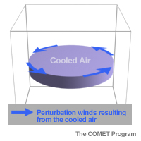
| Suppose the above vortex is filled with a flat cloud deck, the top of which experiences intense radiative cooling. Suppose that
|
The difference between this example and the one above
is that now H=0.5 km, giving 2 400 km >> 70 km, so this feature is dynamically large:
|
Remember, this geostrophic adjustment process is in addition to other forcing. As long as a feature is being forced, it will continue to exist, with its structure evolving as determined by the forcing and gradual modification by the adjustment process. Also remember that vertical shear and horizontal deformation can shred a feature over time, even if the dynamics permit a thermal or wind perturbation to otherwise be retained. This is just one more tool in your bag, not the answer to all forecast problems.
![]()
![]()