3.1.1 Overview
A typical lifespan of a polar low is 12-24 hours, with many dissipating rapidly after landfall. This short
lifespan necessitates a timely response from the forecaster, as the whole event could develop and then decay in
the interval between routine forecasts. Nowcasting of polar low events is therefore of utmost importance to enable
maximum information to be issued to those affected by the event.
Once a polar low has developed, the forecaster is concerned with its behaviour in the next few hours. The three
main questions to be answered are:
1. Will the low deepen further?
2. Where and how fast will it move?
3. When is it likely to
dissipate?
Monitoring the depth of the low in the first place may be difficult unless there are reliable ground based
measurements of wind speed and pressure. In many cases, the forecaster only has satellite imagery and model fields
available for assessing the situation. Given the limitations of these two sources, a knowledge of the structure
and dynamics is necessary to make full use of available data.
3.1.2 Using Surface and Upper Air Observations
According to Rasmussen’s (2003) definition, a small scale arctic low becomes a polar low when the surface
wind speed reaches or exceeds 28 knots.
As the systems are often small and fast moving, careful monitoring of changes in wind speed and direction and
weather conditions at a very few locations can give valuable information. Even with a single observation,
knowledge of the likely wind structure can assist in assessing the position of the low's center, the movement of
the low, and the location of the most hazardous conditions.
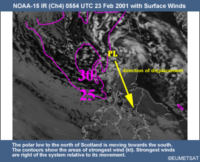
The strongest wind occurs where the circulation flow is in the same direction as the steering flow. This is found
on the right-hand side of the system in relation to its movement. On the left-hand side, winds are likely to be
significantly lighter. On occasions where the low is situated very close to the coast, the circulation may draw in
stable air from the land and actually suppress convective activity very close to the low center. This has been
observed in lows along the Norwegian coast (Noer et al., 2003).
Observations aloft, for example upper air soundings and aircraft reports, can be used to verify the accuracy of
the NWP representation of upper-level systems that drive the polar low. If the upper pattern begins to deviate
from the forecast, then the conclusions drawn from NWP data must be revisited and amended.
3.1.3 NWP Guidance
Many of today's operational models cannot often resolve the small-scale structure of a polar low. However, these
models can give useful information on the large-scale flow in the area. Depending on the intensity and depth of
the system itself, a suitable steering flow for the polar low can be defined. Using a 50-km regional model, Noer
et al. (2003) defined the 700-hPa wind flow as a rule-of-thumb initial guess for the movement of the system.
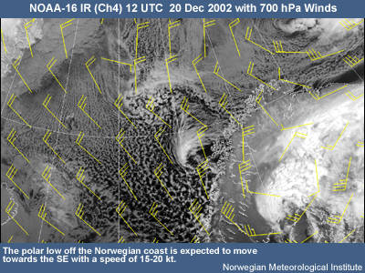
In the example shown, the polar low is clearly seen off the coast of Norway and is embedded in a northwesterly
flow at 700 hPa with strength of around 25-30 knots. It has been observed that the speed of the polar low is
typically 1/3 to 1/2 of the wind strength at this level.
From an analysis of 41 recent polar lows over a four year period, Noer et al. (2003) concluded that the
propogation speed of Norwegian Sea polar lows was usually 15-25 knots, depending on the strength of the background
flow
In reverse-shear situations, the steering flow can be very light, and so the low will be stationary or very slow
moving.
As well as forecasting the motion, NWP fields can be used to determine the likely evolution of the low. In most
cases, the polar low forms due to a combination of a surface disturbance and an upper-air vorticity maximum within
a cold pool or vortex. If the two phenomena remain linked for a period of time after a low forms, it is likely
that the system will remain active for many hours. However, if the upper flow is very mobile and the upper trough
or vortex moves beyond the surface low, the surface forcing alone will not be sufficient to sustain the system,
and it will weaken. Baroclinic polar lows will normally only start to decay when negative dynamic forcing
mechanisms, such as cold air advection or negative vorticity advection, start to play a dominant role.
The accuracy of any NWP-based assessment is dependent on the proper handling of the atmospheric conditions by the
model. If the position, speed, and timing of the features are in error, then the forecast intensity of the low
will also be in error.
Because of the small-scale and rapid development of a polar low, an operational model run may not forecast the
event at all. Once the system has formed, however, the assimilation of satellite data and observations will
encourage subsequent model runs to represent the low. Therefore, new issues of model data should be used as soon
as available to provide the best guidance on the system, as well as the larger-scale forcing mechanisms.
It is useful to determine as far as possible whether a polar low is mainly convectively driven, or baroclinic in
nature. Convectively driven lows will tend to decay rapidly on land- or icefall, whereas a baroclinic system may
persist until dynamic processes inhibit further development.
3.1.4 Satellite Imagery Characteristics
Some useful imagery characteristics to indicate that a low is of sufficient strength to be a polar low are:
1. A clear eye in the center of the system. This only occurs in a few cases, where the upper-level divergence
is stationary in relation to the surface low and encourages the vertical structure to form. The eye thus
indicates a situation where the low has undergone rapid deepening and is likely to be associated with high wind
speeds.
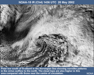
2. Cirrus clouds in a wavelike pattern radiating from the center of the low indicates strong winds.
3. A smooth, non-broken appearance of the upper cloud often indicates a strong polar low, whereas weaker lows
can display individual CBs within the spiral of cloud.
4. Higher cloud-top temperatures near the center, indicating sinking motion.
5. Cloud-top temperatures are typically below -40ºC, and thus reach well beyond the 500-hPa height.
The intensity and structure of a polar low may be deduced through careful analysis of satellite imagery. In the
high latitudes where polar lows are found, however, the coverage of polar orbiting satellites can be patchy. The
usefulness of satellite data depends on the timing and how quickly it is disseminated to the forecaster at the
desk.
In recent years, the availability of satellite-derived wind fields, for example Quickscat winds from ERS-2, can
greatly assist in monitoring the strength of the polar low and defining the areas which are most at risk from
strong winds and icing hazards.
References
Bader, M.J., G.S. Forbes, J.R. Grant, R.B.E. Lilley, and A.J. Waters, 1995: Images in Weather Forecasting.
Cambridge University Press.
Noer, G. and M. Ovhed, 2003: Forecasting of polar lows in the Norwegian and the Barents Sea. Proc.
Ninth meeting of the EGS Polar Lows Working Group, Cambridge, UK.
Online Manual of Synoptic Satellite Meteorology, Central Institute for Meteorology and Geodynamics,
Zentralanstalt für Meteorologie und Geodynamik
(http://www.zamg.ac.at/docu/satmanu4.0/satmanu/manual/PL/pl0.htm)
Rasmussen, Erik A., 1995: Polar Lows News - The Newsletter of the EGS Polar Lows Working Group. June 9, 1995, No
5. Dr. G. Heinemann, Chairman.
Rasmussen, Erik A.and John Turner, 2003: Polar Lows: Mesoscale Weather Systems in the Polar Regions,
Cambridge University Press.