1.2.1 The Polar Low
Nordeng and Rasmussen (1992) called this particular polar low "A Most Beautiful Polar Low." It shows
the classic features of a true polar low:
- The system is relatively small and non-frontal
- Cold air can be seen streaming southward west of the low
- A clear eye appears at the centre of the system. It is this clear area that helps give rise to the term
“arctic hurricane” that is often seen in the literature; for example, in Emanuel and Rotunno (1989).
- The northern spiral arm separates cold air streaming off the ice surface from a modified cold air mass with
open cellular convection
The European Polar Lows Working Group (EPLWG) published the following definition of a polar low at their June
1994 meeting in Paris:
"The term 'polar mesoscale cyclone' is the generic term for all meso-alpha (200 - 2000 km) and meso-beta
(20 - 200 km) cyclonic vortices poleward of the main polar front. The term 'polar low' should be used for
intense maritime polar mesoscale cyclones with scales up to 1000 km with a near surface wind exceeding 15 m/sec
(30 knots)."
A more up-to-date definition by Rasmussen and Turner (2003) states:
"A polar low is a small, but fairly intense maritime cyclone that forms poleward of the main baroclinic
zone (the polar front or other major baroclinic zone). The horizontal scale of the polar low is approximately
between 200 and 1000 kilometres and surface winds near or above gale force."
Rasmussen (1994) suggested classifying polar lows into primary and secondary types. The primary type are those
initiated as the result of a cold core vortex. Those associated with all other vortices that fit the definition of
a polar low belong in the secondary category.
The majority of polar lows seen in Canadian waters fall into the primary category. However, there are some
vortices in which baroclinic processes appear more important than convection during the mature phase, and these
would fall into the secondary category. Some of the vortices forming along the ice edge of southern Davis Strait
appear to fall in this secondary category.
European cases are often a result of pre-existing baroclinic effects and are therefore of the secondary category.
Occlusions from mature synoptic-scale lows are a favoured mechanism between the British Isles and southern
Greenland, while primary polar lows are generally confined to the area north of Iceland across to the Barents Sea.
1.2.2 Examples of Polar Lows
Here are two examples of polar lows in the Labrador Sea and the Gulf of Alaska.
The cloud pattern accompanying the Labrador Sea polar low is common for systems developing in the northwestern
portions of the Labrador Sea. In their paper "Labrador Sea Polar Lows," Rasmussen et al. (1996) studied
a number of Labrador Sea polar lows, all of which tended to form in the same general area and develop
characteristic cloud patterns. The main features are the cloud bands northward and eastward from the centre. The
eastward band or tail frequently marks a boundary between colder arctic air to the north and modified arctic air
flowing eastward on the southern side of the system.
1.2.3 The Comma Cloud
The term "comma cloud" is used to describe a variety of comma-shaped cloud systems both over water and
land. In this discussion it is used to describe comma-shaped cloud patterns poleward of the northernmost jet
stream.
 with overlay
  hide overlay
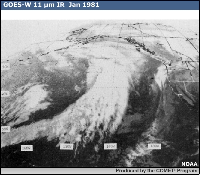
Zick (1983) shows the typical relationship between a comma cloud and a major frontal cyclone. Here, the satellite
imagery is of the northeast Pacific with the comma cloud positioned west of a main frontal zone that is visible
over the Alaskan Panhandle, British Columbia, and Yukon
Mullen (1983) refers to an earlier report by Anderson (1969) in which he first pointed out that a cold air comma
cloud is:
- Invariably downstream of an upper-tropospheric vorticity maximum
- In a region of 500-hPa vorticity advection
- Ahead of a shortwave trough or in the left exit region of a jet
Businger and Reed (1989) add that the comma cloud typically begins as a region of enhanced convection and
geographically is most likely to be observed over the western oceans in areas where cold air is being advected
over warmer water surfaces.
Reed (1979) makes the following comments about comma clouds:
- The dimensions of the comma-shaped cloud patterns are typically of the order of 1000 km in the direction
normal to the southern front and 500 km in the parallel direction
- In cases of multiple systems, 1000-1500 km is a typical spacing
- A surface pressure trough lies under the trailing edge of the comma tail and, in the more intense cases, a
surface low pressure center lies under the comma head
- Wave cyclones are initiated when the disturbances approach sufficiently close to the main frontal band
- The notch of the comma lies in the region of strong horizontal shear on the poleward side of the jet stream
axis at 500 hPa
- The comma lies in a region of appreciable baroclinity, on the cold side of the baroclinic zone where the lapse
rate is conditionally unstable through a considerable depth
1.2.4 The Instant Occlusion
(click to view animation in separate browser window - 489 kb)
If the distance between the comma cloud and frontal wave becomes small enough, the two features may combine with
the resultant cloud closely resembling that of a mature occluded cyclone (Mullen, 1983). This time series over the
Gulf of Alaska at 1845 UTC shows a comma cloud in the cold air mass north of the main frontal band. Nine hours
later, at 0545 UTC, there is an indication of a weak wave developing on the main front. The comma cloud then
proceeds to merge with the main front over the next 24 hours.
This process represents explosive cyclogenesis on a scale much larger than polar low vortices.
1.2.5 Reverse-Shear Flow
Vortices and polar lows are often observed to form in an area of reverse shear. Reverse shear refers to the
situation in which the storm motion is in the opposite direction to the thermal wind. This is unlike the situation
that prevails with the comma cloud type, which propagates in the direction of thermal wind (Businger and Reed,
1989). Duncan (1978) was the first to identify the reverse-shear case and showed that baroclinic development is
favoured in regions of reversed shear.
In forward shear the colder air lies to the left of an observer positioned with his/her back to the wind. The
thermal wind is positive and the actual wind increases with height. In a reverse-shear flow, warmer air lies to
the left of an observer facing downwind. This produces a negative thermal wind, and the actual wind will decrease
with height.
In both cases, the upward motion and comma-shaped cloud pattern are located where the thermal wind advects
positive vorticity (i.e., down-shear of the trough). Because of the opposite relationships between thermal winds
and steering winds, the cloud system lies ahead of the trough in the case of forward-shear and to its rear in the
case of reverse-shear flow.
Reed and Duncan (1987) followed a series of disturbances that formed during a two-day period in January 1983. The
disturbances were spaced about 500-600 km apart and moved southwestward at 10 knots. These lows were steered
southwestward in conformity with the low-level winds. These winds were strongest near the surface where the
thermal gradient was also strongest.
1000 hPa 850 hPa 700 hPa 500 hPa
From the orientation of the isotherms on the 1000-hPa and 850-hPa charts, it is apparent that the thermal wind is
directed opposite to the low-level flow. Note that at these heights, the colder air lies to the right of an
observer facing downwind, and the actual wind decreases with height.
Conditions for reverse-shear flow are not uncommon in the northern Labrador Sea and Davis Strait. When
synoptic-scale lows pass south of Greenland they often develop a surface trough northward along the west Greenland
coast. During the winter months this can produce a situation where the surface flow is closely oriented to the ice
surface. This aids in the formation of a low-level baroclinic zone along the ice edge. Businger and Reed (1989)
and Rasmussen (1994) state that these boundary-layer fronts, separating modified and unmodified air, appear to
play a significant role in the development of baroclinic vortices. Although many remain weak circulations, others
may develop into polar lows if they receive significant upper forcing.
A similar reverse-shear situation can be found at times north and east of Iceland. Here, arctic air flow at the
surface is opposite to the direction of the thermal wind in the lower atmosphere. Any disturbance at the lower
levels, including polar lows, tends to move slowly. If the pattern is persistent, then several shallow
disturbances can develop over the course of a few days.
1.2.6 Shear Vortices and Lines of Enhanced Convection
A uniform flow of cold air is seldom sufficient and perhaps never sufficient by itself for development of true
polar lows. Øakland (1989) says that for convection to be the energy source there must be spatial
variations. The presence of a capping inversion is also necessary as it prevents deep convection from becoming
widespread. The deep convection is then confined to or focused on the area immediately beneath the forcing
mechanism.

This series of vortices over the Labrador Sea formed along a frontal zone. This frontal zone separates cold
arctic air streaming southward behind a synoptic system southeast of Greenland from a warmer air mass that has
moved around this low and lies in a surface trough extending from the low upward along the west Greenland coast.
This image shows cold air streaming across the Labrador Sea behind a major synoptic system that has moved east of
Greenland. The change from shallow to deeper convection is obvious as the air moves further from the ice edge and
the cloud pattern becomes open cellular. The flow appears fairly uniform. But an area of weak convergence and
enhanced convection is evident downstream of the arrows. Interestingly, this area corresponds to the section of
the Labrador Sea that experiences the highest frequency of polar low development. The cases by Rasmussen et al.
(1996), Moore et al. (1996), and Mailhot et al. (1996) all formed in this general area.
Rasmussen et al. (1996) refer to a low-level jet that often develops because of the flow through Hudson Strait
and extends over the Labrador Sea. This feature is often visible as streamers emanating from the adjoining capes.
Small vortices are occasionally observed along the streamers.
Rasmussen (1996) also mentions the effect that the Torngat Mountains may play. Being a relatively high range,
cold air over Labrador will have a tendency to flow around this feature. The flow south of the mountains is nearly
westerly. The flow in the area to the north is northwesterly. The enhanced convection appears to be the result of
this geographicaly induced convergence.
1.2.7 Vortices and Convergence Lines
Another area for the formation of vortices is along a boundary layer front formed due to the convergence of air
streams with different over-water trajectories. For example, the eastward extending tail of the Labrador Sea polar
low in this image lies along a frontal zone resulting from the convergence of two arctic air masses with different
over-water trajectories.
Northern European cases are often preceded by the presence of convergence lines or isolated baroclinic zones that
give rise to an organized pattern of convection. Vortices can sometimes be seen at the boundary between air from
different origins. Usually, a line of bright cloud tops is observed, as in this example.
References
Anderson, R.K., J.P. Ashman, F. Bittner, G.R. Farr, E.W. Ferguson, V.J. Oliver, and A.H. Smith, 1969:
Applications of meteorological satellite data in analysis and forecasting. ESSA Tech. Rep. NESC 51 [NTIS AD-697
033].
Bader, M.J., G.S. Forbes, J.R. Grant, R.B.E. Lilley. and A.J. Waters, 1995: Images in Weather Forecasting.
Cambridge University Press.
Businger, S. and R. Reed, 1989: Cyclogenesis in cold air masses. Wea. Forecasting,
4. No. 2, 133-156.
Duncan, C.N., 1978: Baroclinic instability in a reversed shear flow. Meteor. Mag. 107, 17-23
Emanuel, Kerry A. and Richard Rotunno, 1989: Polar lows as arctic hurricanes. Tellus, 41A, 1-17.
Mailhot J., D. Hanley, B. Bilodeau, and O. Hertzman, 1996: A numerical case study of a polar low in the Labrador
Sea. Tellus, 48A, 383-402.
Moore, G.W.K.., M.C. Reader, J. York, and S. Sathiyamoorthy, 1996: Polar lows in the Labrador Sea: A case study.
Tellus, 48A, 17-40.
Mullen, S., 1983: Explosive cyclogenesis associated with cyclones in polar air streams. Mon. Wea. Rev.,
111, 1537-1553.
Noer, G. and M. Ovhed, 2003: Forecasting of polar lows in the Norwegian and the Barents Sea. Proc. Ninth
meeting of the EGS Polar Lows Working Group, Cambridge, UK.
Nordeng, Thor Erik and Erik A. Rasmussen, 1992: A most beautiful polar low: A case study of a polar low
development in the Bear Island region. Tellus, 44A, 81-99.
Øakland, Hans, 1989: On the genesis of polar lows.Polar and Arctic Lows. Twitchell, P., E.
Rasmussen, and K. Davidson, Eds., A. Deepak Publishing.
Parker, Neil, 1997: Cold Air Vortices and Polar Low Handbook for Canadian Meteorologists. Environment
Canada.
Rasmussen, Erik A.and Anette Cederskov, 1994: Polar lows: A critical analysis. The Life Cycles of Extratropical
Cyclones, Vol. 111. Proc. of an International Symposium, Bergan, Norway.
Rasmussen, Erik A., 1995: Polar Lows News - The Newsletter of the EGS Polar Lows Working Group. June 9,
1995, No. 5, Dr. G. Heinemann, Chairman.
Rasmussen, Erik A., Chantal Claud, and James F. Purdom, 1996: Labrador Sea Polar Lows. The Global Atmosphere
and Ocean System, Vol. 4, 275-333.
Rasmussen, Erik A.and John Turner, 2003: Polar Lows: Mesoscale Weather Systems in the Polar Regions,
Cambridge University Press.
Reed, R., 1979: Cyclogenesis in polar air streams. Mon. Wea. Rev., 107, 38-52.
Reed, R. and C. Duncan, 1987: Baroclinic instability as a mechanism for serial development of polar lows: A case
study. Tellus, 39A, 376-384.
Zick, 1983: Method and results of an analysis of comma cloud developments by means of vorticity fields from upper
tropospheric satellite wind data. Meteor. Rundsch. 36, 69-84.