This is the print version of the Conceptual Models of Tropical Waves webcast, presented by Mr. Horace Burton and Mr. Selvin Burton under the auspices of the MeteoForum Project.

Mr. Horace Burton is Chief Meteorologist at the Caribbean Institute for Meteorology and Hydrology, and lectures Meteorology at the University of the West Indies. Mr. Burton has over 25 years of experience in meteorology, including forecasting in the tropics.

Mr. Selvin Burton is Chief of Data and Information Services at the Caribbean Institute for Meteorology and Hydrology, and senior lecturer in Meteorology at the University of the West Indies. He has been involved as a meteorologist for over 25 years in both operational forecasting and research, as well as teaching.

Module description and objectives

This module examines some Conceptual Models of Tropical Waves, particularly those that affect the eastern Caribbean. Tropical waves are prolific rainfall producers that sometimes form tropical cyclones. Conceptual Models of Tropical Waves are used to help learners understand the dynamical characteristics and evolution of tropical waves. Users will learn about the vertical and horizontal structure of tropical waves and the typical weather changes that accompany the passage of a tropical wave. Four different methods of tracking tropical waves are also provided.

After completing this Webcast, users should be able to:

• Define tropical waves and state why they are important
• Describe the typical wavelength, frequency, propagation speed, and direction of tropical waves
• Describe the horizontal structure and vertical structure of tropical waves in terms of winds, moisture and temperature
• Describe the lifecycle of Reihl's Classical easterly wave in terms of wind velocity, relative humidity, clouds, and precipitation
• Identify tropical waves based on Frank's Inverted 'V' model, i.e., banded clouds in the shape of an inverted 'V'
• Describe the relationship between the upper and lower troposphere flow in Frank's conceptual model
• Describe the characteristics of African waves including their origin, wavelength, and relative intensity between inland and the coast
• Describe the typical distribution of divergence in African waves
• Describe the distribution of vorticity in African waves
• Describe the distribution of clouds and precipitation in African waves
• Understand that inter-annual variations in the frequency and strength of African waves are correlated with the occurrence of intense Atlantic storms
• Detect and track tropical waves using satellite imagery, satellite-derived surface winds, wind profiles, and model output

Click here to start the animation.

Westward-propagating wave disturbances are the source of many tropical cyclones. Most of the waves in the Atlantic and the Caribbean have their origin over Africa. Observations indicate that perturbations in the low-level easterly flow occur as a result of a variety of circumstances. The term tropical wave is sometimes used to describe these different systems, which can be prolific rainfall producers and are also associated with strong winds and flooding.

One definition of a tropical wave is a trough, or cyclonic curvature maximum, in the trade wind easterlies. These may reach maximum amplitude in the lower or middle troposphere, or may be a reflection from the upper troposphere of a cold low, or the equatorward extension of a mid-latitude trough. In some cases they can also be a poleward inflection of low-level cyclones in low latitudes.

In terms of general characteristics, these are basically synoptic-scale systems with considerable latitudinal extent, about 10 to 15 degrees latitude. They exist apart from the ITCZ, although they may extend into that area. Their wavelengths are of the order anywhere from 1500 to 3000 km and generally move westward at between 5 and 10 m s^-1, equivalent to 10 to 20 knots, and they have a frequency in the peak season of about one every 3 to 4 days. They are most intense between 850 and 700 hPa; that’s where they reach their maximum amplitude and they’re generally cold core up to about 600 hPa with a weak warm core above, and generally they slope eastward with height.

This diagram illustrates the horizontal view of a wave. The dashed lines are the isobars at the surface and the red lines are streamlines at 700 hPa. You can see the wave at the surface in the isobar pattern with the winds from the east and east-southeast behind the wave axis, and east-northeast and northeasterly ahead of the wave axis. The wave axis is indicated by the white lines at the surface, and here again at 700 hPa, you can see that the axis of the wave at 700 hPa is to the east of the wave at the surface, showing the eastward tip. This diagram is also an indication of a small cyclonic circulation at 700 hPa, which indicates a typical or strong wave. We do find circulation at 700 hPa even though there is no circulation at the surface.

This is an illustration of vertical cross section showing the wind structure across the wave. The curved black line is the wave axis, with the tilt to the east. You can see that in this case the wave extends up above 20,000 feet (6,000 meters). You can see the wind structure with winds basically east-northeast, northeasterly, and even northerly ahead of the wave, and east-southeast and southeasterly behind the wave. Again, you can see that the greatest curvature occurs not at the surface, but somewhere between 5000 and 10,000 feet (1,500 to 3,000 meters) and between 850 hPa and even 700 or 600 hPa.

Satellite imagery indicates that the cloud and precipitation patterns may differ significantly from one wave to another. Various wave models are used to describe the different wave patterns.

In the sections that follow of this module we will examine 3 models: Riehl’s Classical Easterly Wave Model, Frank’s Inverted “V” Wave Model, and the African Wave Model.

The first model we’ll look at is Riehl’s Classical Easterly Wave model. We refer to it as “classical” because it was one of the first models to be developed for the eastern Caribbean. Riehl and associates used upper-air data from the Caribbean and traced the movement of isallobaric centers across the western Atlantic and the Caribbean Sea during the summer. The isallobaric centers turned out to be accompanied by westward-moving, wave-like oscillations in the basic easterly current, in the lower troposphere. That’s why the name wave was given to the model.

This is a depiction of Riehl’s model showing the distribution of wind and a schematic representation of the cloudiness. In a typical case, the area west of the wave axis is characterized by subsidence and fair weather, while areas of convergence and disturbed weather occur east of the axis. You can see the moist layer ahead of the wave, just about 5,000 feet. We can also see that with the passing of the wave, the moist layer becomes much deeper, extending up above 20 to 25,000 feet (6,000 to 7,500 m). You can see that as the wave moves further west, the actual moist layer turns to a depth of about 7,000 feet (2,100 m). Fair weather cumulus, and some cumulus congestus and altocumulus ahead of the wave, where you can see showers and thundershowers, and cumulonimbus clouds with the passage of the wave.

We just saw a schematic representation of Riehl’s model. Here we have an actual situation, from Riehl’s theory, in 1948, where a wave passes across the eastern Caribbean. You can see that here the structure of the wind looks quite similar to the schematic representation, with the largest curvature occurring between 5,000 and 10,000 feet (1,500 to 3,000 m). With the passage of the wave, the wind shifts from east-northeasterly to southeasterly or east-southeasterly. The letter C here represents areas where basically we are getting convergence; ahead of the wave there will be divergence. Based on this plot, we can see the amount of cloudiness increasing with the passage of the wave, becoming cloudy and overcast behind the wave, with thundershowers, rain, cumulonimbus clouds, showers, and thundershowers and rain being reported after the passage of the wave.

The following sequence will give you a general idea of the typical cloud and precipitation patterns associated with these systems.

In the ridge, which is ahead of the trough, we normally find trade wind cumulus of average height, no precipitation, which is why we see shallow cumulus.

Clouds and precipitation ahead of the trough: As we get close to the cloud axis, the cumulus height or depth increases to become above-average development. We tend to get some cirrus and altocumulus, and the visibility tends to improve. A few, very light showers may occur as the trough line approaches.

Clouds and precipitation close to the trough axis: At the trough line itself, the cloud structure becomes more complex, and cumulus congestus or cumulonimbus clouds start to develop. Cirrus and altocumulus continue, and the frequency and intensity of the showers increases with the passage of the trough line, or the wave.

Clouds and precipitation at the trough axis: As the axis passes, the cumulus congestus and the cumulonimbus clouds become more frequent, and we see the development of layers of stratocumulus, altocumulus and altostratus clouds, and cirrus and cirrostratus. Shower activity becomes more frequent, with moderate to heavy showers and thundershowers, and light rain between those showers.

Clouds and precipitation at the rear of the trough axis: As the wave progresses westward, shower activity tends to decrease and cloudiness and precipitation will gradually decrease; we return to the situation of being on the ridge, and now we see the normal fair weather associated with those systems.

The next model is Frank's inverted "V" model. This is based on some work done by Neil Frank in the 1960's, published in a paper in 1968. Satellite imagery was used to look at the cloudiness associated with some systems in the Atlantic during the 1960's, and it was found that the cloudiness associated with some systems was arranged in bands which seemed to be arranged with a pattern resembling a nested series of upside-down or inverted "Vs" that are envisioned in Frank's model.

This is part of the intertropical convergence zone, a schematic representation of what the wave would look like. You can see these bands here that look like an upside down "V", with some cloudiness, in this case cumulus and stratocumulus, in these bands. Now, in general, the clouds appear as bands arranged in the form of an inverted or upside down "V" which are considerably flattened or rounded.

In many cases, the number of bands or "Vs" may vary from one case to another, and in some cases, if not most, you may only find part of an inverted "V", not necessarily the entire "V".

In a very well marked pattern, the axis of the wave is coincident with the apex of the "V" and indicates the place where the bands change the orientation.

The cloud bands tend to be aligned parallel or nearly parallel either to the lower tropospheric winds or to the shear, usually being more closely aligned to the low level wind shear than to the flow at any one level. The cloud organization is on a synoptic scale covering an area of about 2500 km², extending anywhere from about 5 to 25 °N, and persisting for several days.

Outside of the intertropical convergence zone (ITCZ), much of the cloudiness consists not of hot towers, or cumulonimbus clouds, but stratocumulus, cumulus, and perhaps some isolated towering cumulus. Convective activity is relatively sparse, a rather typical feature of these systems. The system, the inverted "V" itself, tends to be best defined in the eastern and central north Atlantic, but becomes less distinct as it moves westward and generally disappears before reaching the Lesser Antilles or the eastern Caribbean.

This is a depiction of the cross section showing the wind profiles from Dakar and some across the eastern Caribbean which Frank used to track these waves from Dakar to the eastern Caribbean.

You can see the actual shift of the wind from east-northeasterly to southeasterly or east-southeasterly wind.

These cross sections that Frank used to track the waves across the Atlantic to the eastern Caribbean show a number of waves that were tracked from Dakar across the Caribbean. This particular wave, for example, moved off Dakar about the end of July, and reached the eastern Caribbean somewhere around the 10th of August.

This is an actual satellite image showing an inverted “V”. In this case we can see just one inverted “V”, although there is some indication of another inverted “V” below 10 degrees north. The main flank of the wave here is between 10 and 15 degrees north. Note in this picture there is not a lot of deep convection, mainly stratified cumulus clouds.

Frank found that although the cloudiness generally decreased as the waves moved westward, a temporary enhancement of what he called a blow-up in the cloudiness often occurred over the eastern Caribbean, and this caused some concern for him in his work. His examination of the 200 hPa pattern revealed that the temporary blow-ups, which typically lasted for only a day, usually occurred as the waves moved under the southeastern quadrant of an upper level trough or low.

This schematic diagram shows the mid-Atlantic trough, which is persistent across the eastern Caribbean during the summer. What Frank found was that for cases where waves blew up, most of the time the increase in cloudiness occurred when the waves moved under the influence of the southerly or southwesterly flow ahead of the upper-level trough.

Frank suggested that this is the result of interaction with the upper-level trough, to the east of which we have upper-level divergence that actually influences or enhances the low-level convergence and causing the increase in convection that takes place with the blow-up. In fact, Frank suggested that Riehl's model is not a low-level system by itself, but actually the enhancement of the low-level system by the upper-level trough, so that Riehl's model is really the interaction between the low-level system (the wave) and the upper-level trough that provided the upper-level divergence to enhance the low-level convection.

As we said, most of these waves form over Africa and they tend to form somewhere between 15 and 30 °E. These synoptic scale systems are similar to those we find in the Atlantic and over the eastern Caribbean, with latitudinal extents of 10 to 15 degrees. They generally do not have an associated surface vortex until they reach the vicinity of the African coast, and they attain their maximum amplitude and intensity near the coast. The majority of these systems tend to weaken somewhat as they progress westward from the African coast, although they may intensify in the Atlantic and the Caribbean Sea and become tropical cyclones.

The cloud patterns associated with these systems are either circular or banded, they are usually poorly defined inland but become recognizable and coherent before reaching the coast. Rainfall is usually widely scattered east of the Cameroon mountains, anywhere between about 10 to 12 °E, but actual cloudiness increases as the systems intensify.

Low-level convergence occurs ahead of the wave axis, while behind the wave axis we see divergence. Notice that this pattern actually is reversed at 700 and 200 hPa, where intense areas of divergence and convergence are observed above the regions of low-level convergence and divergence, respectively. This pattern of low-level convergence ahead of the wave and divergence behind the wave is opposite to what is associated with the Riel’s Classical Easterly Wave model.

Strong, low-level cyclonic vorticity occurs ahead and across the wave axis, with the strongest values at about 800 or 700 hPa, along what is called a reference latitude, at around 10 °N.

Strong rising motion occurs ahead of the wave, in the vicinity of the cloud and the precipitation maximum, and the maximum rainfall and thunderstorm activity tend to occur some distance ahead of the trough.

One of the characteristics we find with these systems is that there tend to be two cyclonic centers, which occur over the African continent. One of them occurs near 20 °N, in the confluence zone between the moist air to the south and the dry Saharan air to the north. The second center is located between 10 and 12 °N, in the area of the convective cloud maximum, and the pressure fluctuation of 3 to 4 hPa with the northern eddy compared to a fluctuation of less than 1 hPa to the south. The actual system to the north is more associated with the heat low, while the actual system to the south is the one that is associated with the wave itself.

This is an example from Carlson’s paper in 1969 showing what the actual system may look like. This is satellite imagery, and here are surface isobars, 2,000 foot wind (600 m), and 10,000 foot wind (3000 m), and you can see that in this particular case there’s a strong cyclonic circulation here at 2,000 feet.

This composite picture from ESSA 5 satellite images is just off the African coast, associated with this area of cloudiness here, which is the actual wave; this is August 25, 1967.

In this section we will consider how we track these tropical waves.

In earlier sections we talked about the characteristics and structure behavior of the waves, but one of the major problems facing the forecaster is tracking them across the Atlantic.

This was particularly true in the early days, in the absence of satellite imagery and other data, because there was little information to go with.

We will explore some of the ways we can now use to actually track the waves across the systems.

One is actual satellite imagery.

We can also use sounder satellite derived winds...

upper air soundings or, as in more recent times...

we look at model output to track these waves across the Atlantic.

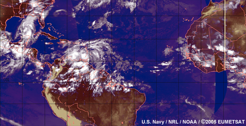
We've talked about satellite imagery, and here is a case in which we can track several waves. We talked earlier about the inverted “V”, and we see a wave out at about 30 °W (number 1) showing just one leg. Over the Caribbean itself there is another wave (number 2), which is interacting with an upper-level trough located somewhere across the Española area. There is not a lot of significant convection associated with this particular wave. And there is probably another wave at about 50 °W (number 3).

This is a QuickSCAT image of surface winds. These images have been quite useful recently to actually track waves. We mentioned earlier the change in wind speed, in this particular case there is a wave axis somewhere between about 35 and 38 °W. We can see the east and east-northeasterly winds and north-northeasterly winds on the front or the western side of the axis and then southeasterly and southern winds on the east side. This is a good example of what would be a very strong wave, strong in the sense that it is a very large cyclonic curvature associated with the system.

We can look at time sections, and this is useful, although in many cases none of these are available across the Atlantic, particularly in the Caribbean. This is a time section for Barbados, where to some extent we can use it as a diagnostic, as well as a forecasting tool. Now this particular case there are a number of wave axes, but we can look at this particular one which is passing through Barbados in September, and we can see here some strong northerly winds ahead of the axis and some southeasterly winds to the west side, northerly winds to the west, and southeasterly winds to the east of the axis, and we can see that this pretty strong wave stretches all the way up to about 700 hPa, where we have a strong curvature.

One of the ways that we recently use to track these waves is to look at the model output and to actually look at vorticity centers. The waves are cyclonic curvature in the wind, and therefore are associated with cyclonic vorticity. We actually look at absolute vorticity and vorticity maxima, and use it to track the waves across the Atlantic. We use models, and therefore we use model output to not only track, but also to forecast these systems across the ocean.

The images in the following section are an example of a case in which vorticity maxima were used to track a wave across the Atlantic. In terms of the models, we have found that in many cases they are rather consistent and a good way of tracking these systems across the Atlantic.

This is a case from June 1997, and we see here out in the eastern Atlantic a wave of vorticity maximum of about 6x10^-5-1. We are going to track this wave across the Atlantic. This is a 12 hour forecast, and we will track this wave across the Atlantic using model output from various days and hours.

This is the 24 hour output from that particular model 12 hours previously, and we can see that the vorticity max is moving slowly toward the west. You notice that even though this is a vorticity max, there is not a large curvature in the winds at 700 hPa, but we do have a vorticity max, because we have easterlies here and just the southeasterly so that there is a very small curvature, but certainly a vorticity field is very well indicated. This is the system, now somewhat not as clearly defined, but a weak maximum, still pushing toward the west, and this is a 36 hour forecast. So you see from this output there is some consistency with the model as it's tracking across from 12 hours out to 36 hours, and 48 hours, and the model now places the wave somewhere in the region of about 45 °W.