Scenario
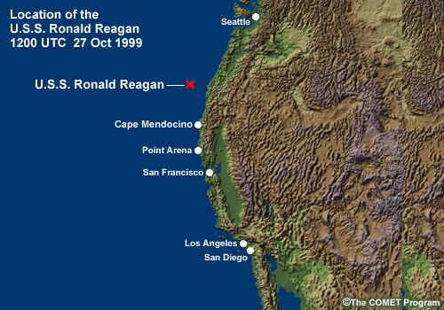
Scenario » Leaving Seattle (1200Z 27 Oct 1999)
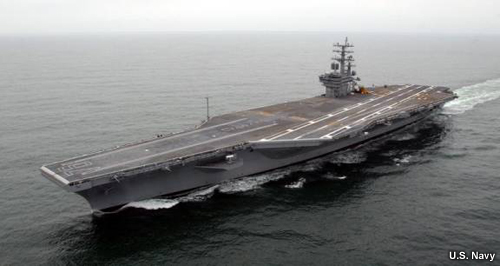
We're aboard the U.S.S Ronald Reagan, an aircraft carrier bound for home. After two weeks in port, getting some work done at the Bremerton Shipyards, near Seattle, we were heading south for San Diego.
Nothing against Seattle, but I miss San Diego. I like my weather warm, my food hot, and my drinks cold. Beats cold drizzle and hot coffee in my book.
Scenario » Storm on the Way (1200Z 27 Oct 1999)
We were only supposed to be in port for a week, but maintenance found some unexpected work to do, so we spent an extra week roaming Seattle. Now we're trying to get ahead of the first storm of the winter and to conduct some training flights as well.
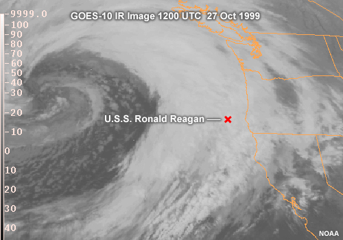
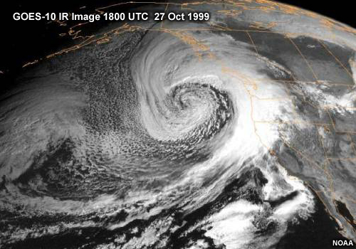
It's 1200Z on 27 October 1999. A look at the satellite loop tells the story. A cyclone 1000 kilometers to the west is heading toward Vancouver Island. We're presently located off the Oregon Coast, getting close to California. Ceilings are already dropping and we're getting sporadic rain. It looks like we won't launch planes until the front passes.
Scenario » Trouble (2300Z 27 Oct 1999)
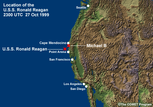
We'd rounded Cape Mendocino and were off Point Arena when we received word of a fishing boat in trouble. According to the Coast Guard, the trawler "Michael B" had apparently lost power and was adrift. The trawler was located just south of Cape Mendocino, in an area known as the Lost Coast. The Michael B had drifted close to shore and was in danger of running aground. We were the closest assistance available. The Coast Guard has dispatched a cutter to the scene and wants to know if we can assist.
The Duty Officer and the CAG (Commander, Air Group) were meeting to discuss options for the rescue. They need a weather briefing. Now.
Scenario » Current Obs (2300Z 27 Oct 1999)
I pull up the latest ship and buoy observations. In the rescue area, winds are running about 25 knots, out of the south-southeast. North of Cape Mendocino, winds are stronger, about 35 knots. But that shouldn't present a problem for us.
Scenario » Forecast (2300Z 27 Oct 1999)
A look at the Eta model winds shows general agreement with the obs. The forecast winds are a bit lighter and come in at more of an angle to the coastline, oriented south-southwest and running about 20 to 25 knots. However, the model forecast indicates the wind speeds should be decreasing over the next few hours.
Looking at the low-level theta-e and wind fields, we can expect the front to pass through at about 00Z. Then conditions should start to improve.
The CAG dispatches 2 helicopters to evacuate the trawler.
Scenario » More Trouble (0000Z 28 Oct 1999)
The helicopters are on the scene and things are getting ugly. Winds are a sustained 45 knots with stronger gusts! Seas are huge. How can that be? How in the world did the model miss that?! Now the CAG is angry that I busted the forecast and his pilots are involved in some risky rescue mission. At this point, I can only hope that everything turns out all right.
Why are the winds so strong out ahead of the front? Why are they parallel to the coast when the model says that they should be coming in at about a 45° angle?
Conceptual Background
Conceptual Background » Discussion
Conceptual Background » Discussion » Conceptual Background
Landfalling cyclones and their attendant fronts significantly impact the structure of mesoscale wind and precipitation fields along the west coast of North America. The complex interaction of the wind field with topography can locally enhance nearshore winds. Destabilization of the atmosphere and the subsequent development of focused heavy precipitation can lead to significant flood events in mountain valleys. While the basic theory governing flow interaction with topography is well known, forecasting wind and precipitation remains a difficult task. The variability of wind, moisture, and temperature within a cyclone, when combined with complex topography, alters the significance and subsequent impact of the interaction.
For more information, see the COMET module Flow Interaction with Topography (https://www.meted.ucar.edu/mesoprim/flowtopo/)
Conceptual Background » Discussion » Description of Topographic Interactions
This visible satellite image shows a well-developed cyclone off the Pacific Northwest. A cold-frontal cloud band makes landfall along the Washington / Oregon coast, then trails offshore farther south. In this typical synoptic situation, southwesterly flow exists ahead of the cold front, changing to northwesterly flow behind it. The environment is typically fairly stable ahead of the front, becoming less stable as the front approaches and perhaps even unstable after frontal passage.
Conceptual Background » Discussion » Basic Conceptual Model
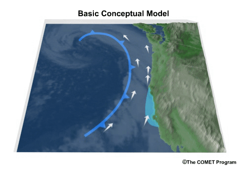
Coastal mountain ranges parallel the West Coast from Southern California up through British Columbia and southeast Alaska. These mountains produce topographic effects on the structure and evolution of fronts and cyclones as they approach the coast. We can summarize the basic effects as follows:
- Alteration of the structure of the wind field. Under stable conditions, the cross-mountain component of low-level flow is blocked. Under less stable conditions the low-level flow moves freely up and over the coastal mountains.
- Locally enhanced along-coast winds, which may occur under both blocked and unblocked conditions.
- Localized pressure gradients and ageostrophic circulations that develop and intensify as fronts make landfall. Alteration of the wind field sometimes develops well ahead of the front, but may occur postfrontally as well.
- A slowing of the landward movement of fronts and their associated precipitation fields.
- Enhancement of precipitation on the windward slopes of coastal mountains as flow ascends the barrier.
Conceptual Background » Discussion » Modification of Coastal Winds by Topography
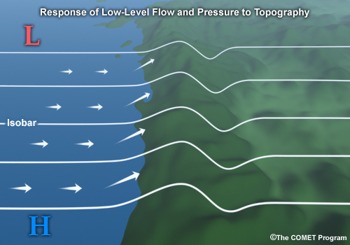
As fronts and cyclones approach coastal mountains, the wind exhibits a strong tendency to turn in an along-mountain direction and often increase in speed. This diagram describes the dynamic response as a front approaches a mountainous coastline from the west. Low pressure sits to the north and west. The flow well offshore is mostly geostrophic, flowing nearly parallel to the isobars and directed onshore. As the front approaches, there can be a variety of responses depending on several factors, including wind speed and wind direction, the height and orientation of the coastal mountains, and the stability of the lower atmosphere.
The Froude number is one parameter that accounts for several of these factors. The Froude number (Fr) is merely the cross-mountain component of the wind (U) divided by the stability (N = Brunt-Vaisala Frequency) times the mountain height (h): Fr = u/ (N * h). From this you can see that increasing wind speed increases the Froude number while increasing stability or mountain height decreases the Froude number.
For more information and to gain more familiarity with the Froude number complete the Froude Number Exercise or review the module Flow Interaction with Topography (https://www.meted.ucar.edu/mesoprim/flowtopo/).
Conceptual Background » Discussion » Froude Number Exercise
Question 1
Use Froude Number Calculator.To explore what variables control the Froude number, and their effects on the wind field, let us examine some reasonable scenarios for the U.S. West Coast. The coastal mountains generally range in height from 1000 to 1500 meters, so let's start with 1500 meters. As a cyclone approaches, we might expect southwesterly flow of 25 knots. Then let's assume a lapse rate of 6.5°C/km, a value close to the standard atmosphere. Under these conditions, will the low-level flow be blocked, or will it ascend and pass over the coastal mountains? (Choose the best answer.)
The correct answer is b).
With mountains of 1500 meters, southwesterly flow of 25 knots (or about 12 m/s), and a lapse rate of 6.5°C/km, you should calculate a Froude number less than one. The greatest uncertainty in this case is the angle between the flow and the ridgeline. Along the U.S. West Coast, the orientation of the mountains varies from north-south in the north, to east-west for parts of southern California. However, over most of its length, the coast trends north-northwest, which yields a flow/ridge angle of about 60° to 70°. Combined with the other conditions, this yields a Froude number in the range of 0.65 to 0.70.
Question 2
Use Froude Number Calculator.Frequently along the west coast, we find a cool marine layer capped by an inversion. For the sake of this exercise, let's assume that means an isothermal layer of 10°C. If a sea breeze developed along the coast with a cross-mountain windspeed of 20 knots (10 meters per second), how high a ridge could it ascend? (Choose the best answer.)
The correct answer is c).
Flow is 10 meters per second perpendicular to the ridge. The lapse rate is 0°C/km. If the mountains are 1000 m high, then the Froude number is a measly 0.54 — far too low to attain the ridge. If we reduce the mountain height until the Froude number equals 1, we find an elevation of just over 500 meters. Thus, the sea breeze will rarely pass over the mountains.
Question 3
Use Froude Number Calculator.As we will see later in this module, after a front passes, the winds tend to turn more westerly and the atmosphere destabilizes, with lapse rates approaching 9°C/km. What wind speed is required for the low-level flow to ascend and pass over the mountains under these circumstances? (Choose the best answer.)
The correct answer is b).
With a 60° to 70° angle between the wind and the ridgeline and a lapse rate of 9°C/km, a wind speed of 10 m/s, or roughly 20 knots, is required to ascend a 1500 m high ridge. Thus, we don't expect much flow blocking after a front passes.
Conceptual Background » Discussion » Stable Flow (Fr < 1)
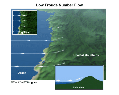
If the cross-mountain wind component is small and/or the air mass is very stable, the Froude number is less than one. Under these conditions the low-level flow cannot ascend the ridge and is blocked. Then the flow below mountaintop level in the coastal zone is forced to turn toward low pressure and accelerate in the along-coast direction. This flow blocking produces a distinct barrier jet below mountaintop level, similar to that observed in cold air damming or other blocked flow situations. The amount of along-coast acceleration is determined by the magnitude of the pressure gradient along the mountain barrier. Because the flow partially ascends the windward slope before its ascent halts, the blocked flow tends to be cooler than air further offshore. Consequently, the blocked region has slightly higher surface pressure, which results in what appears as a windward ridge.
Windward ridging is especially prevalent when cold interior air can be advected out through coastal gaps into the blocked flow. This event occurs frequently during winter months when cold interior air is drawn toward the coast as pressure falls in response to an approaching cyclone.
As with other flow blocking scenarios, the upstream or offshore distance impacted by the blocking is determined by the Rossby radius associated with the topography. Under stable conditions at midlatitudes, the Rossby radius is typically on the order of 1000 km.
Conceptual Background » Discussion » Less Stable Flow (Fr > 1)
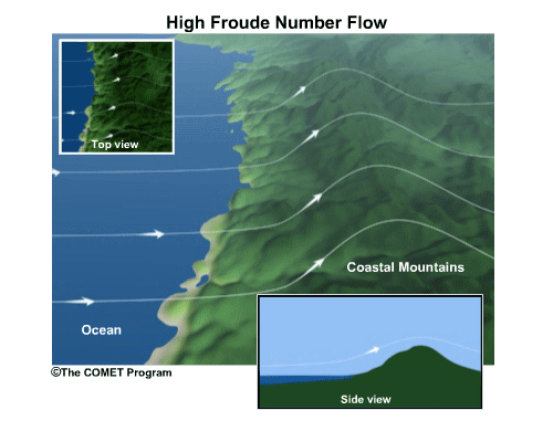
Even when the flow is not totally blocked (Fr > 1), the wind still tends to turn toward low pressure and blow more parallel to the mountain barrier. In this situation, adiabatic cooling in the air being forced up the mountain acts to produce a windward ridge of higher pressure on the upwind side of the mountain barrier. Adiabatic warming of descending air on the downwind side produces a lee trough. In response, the flow slows as it ascends the mountain range and turns across isobars toward low pressure, trying to adjust to the windward ridge. The magnitude of the response depends on the magnitude of the windward ridging, which depends on the background stability and incident flow speed. Moderately strong stability with strong flow across the topography will produce a more pronounced windward ridge.
The along-coast wind response can be highly variable up and down the coast due to variations in both the background pressure gradient as well as variations in the dynamically forced pressure field discussed previously. The maximum dynamic response tends to occur when the Froude number equals one about midway up the mountain. This results in blocked flow at low levels, but not near ridgetop level. Consequently, flow blocking and windward ridging can contribute to along-mountain flow acceleration.
Conceptual Background » Questions
Conceptual Background » Questions » Question
Question 4
Which conditions lead to a high Froude number? Use the pull-down menu to choose the best answer.
The correct answers are highlighted above.
The Froude number (Fr) = U / (N * h). Thus, a high wind speed perpendicular to the mountain, low stability, and a low ridgeline contribute to a high Froude number, which allows the flow to pass over the mountain barrier.
Conceptual Background » Questions » Question
Question 5
[T/F] High wind speed leads to a high Froude number. (Choose the best answer.)
The correct answer is False.
It is the wind component oriented perpendicular to the ridge that is used to determine the Froude number. Thus, a strong wind blowing parallel to the ridge may have a component perpendicular to the ridge that approaches zero, which leads to a very low Froude number. In addition, very stable conditions and high mountains act to decrease the Froude number. Consequently, a high wind speed does not automatically lead to a high Froude number.
Conceptual Background » Questions » Question
Question 6
[T/F] Flow with a high Froude number is not deflected toward low pressure as it crosses a mountain ridge. (Choose the best answer.)
The correct answer is False.
As air ascends the ridge, it cools at the adiabatic lapse rate. The lifted air is typically cooler than the surrounding air mass, which leads to a windward ridge. The formation of a windward ridge tends to result in a deflection of the flow toward low pressure. In the case of a landfalling front along the U.S. West Coast, this will be a deflection toward the north.
Conceptual Background » Questions » Question
Question 7
Where would you expect to find greater low-level stability in the marine environment? (Choose the best answer.)
The correct answer is a).
The prefrontal environment tends to exhibit greater stability. Warm advection from lower latitudes typically increases stability. This occurs because the warm advection is not uniform; higher wind speeds aloft lead to greater warm advection aloft. Warming aloft decreases the lapse rate, which increases the stratification and stability of the atmosphere.
Conceptual Background » Questions » Question
Question 8
Which of the following effects are associated with flow blocking in a prefrontal environment? (Choose all that apply.)
The correct answers are a), b), and c).
When flow is blocked in a prefrontal environment, several things may occur. First, the incident flow turns toward low pressure and accelerates. This may lead to a barrier jet. Second, cooler air pooled along the coastal mountains leads to a windward ridge. And third, the wedge of cool trapped air impedes the forward progress of the front. We explore these and other effects through case examination in the following sections.
Modification of the Prefrontal Wind Field
Modification of the Prefrontal Wind Field » Case Example: 7 Jan 1995
Modification of the Prefrontal Wind Field » Case Example: 7 Jan 1995 » Synoptic Setting
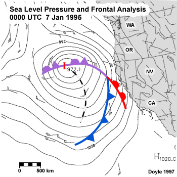
This figure shows a surface analysis for 0000 UTC 7 January 1995 with a typical synoptic setting for a cyclone and attendant fronts approaching the West Coast. As the fronts near the coast, interaction with the coastal topography results in the development of a barrier jet.
Modification of the Prefrontal Wind Field » Case Example: 7 Jan 1995 » Development of Low-Level Stratification
Question 9
This figure shows a mesoscale analysis of the fronts and the 900-hPa theta-e field for the same time as the previous synoptic chart.
On the image below:
- Use the pen to mark where you see warm air advection occurring.
When you have finished, select Done.
Compare your answer to the answer below.
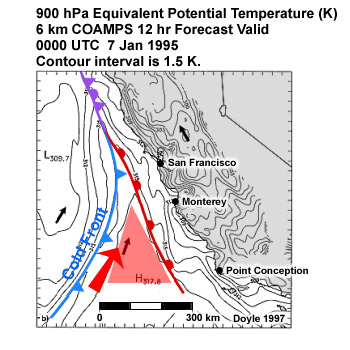
Note the tongue of high-theta-e air. This indicates that there is strong, low-level, warm, moist advection from the southwest ahead of the cold front. However, this warm advection is not uniform. Stronger winds above the surface lead to increased warm advection at higher levels than at lower levels. This differential warm advection acts to increase the stratification as the front approaches. Increasing stratification increases the stability, which in turn, decreases the Froude number. The result is blocking of the low-level, cross-mountain wind ahead of the cold front.
Modification of the Prefrontal Wind Field » Case Example: 7 Jan 1995 » Development of Barrier Jet
Question 10
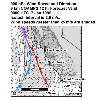
This plot shows the 900-hPa winds at the same time as the previous plots. This roughly corresponds with mountaintop level or just below along much of the California coast. How would you characterize the flow about 200 km offshore from Monterey, in the center of the figure? (Choose the best answer.)
The correct answer is a).
The 900-hPa winds shows SSW flow near mountaintop level that impinges on the coast at about a 45° angle. This occurs even though the flow is deflected northward as it approaches the coast. Experience shows that a 45° angle between the flow and the mountains maximizes the interaction with the coastal topography in both blocked and partially blocked situations. In response to blocking of the low-level flow, the winds turn parallel to the coast and accelerate toward lower pressure, to the north-northwest.
Modification of the Prefrontal Wind Field » Case Example: 7 Jan 1995 » Barrier Jet
Question 11
This cross section shows isotachs of the along-coast wind component.
On the image below:
- Use the pen to mark the highest velocities on the plot.
When you have finished, select Done.
Compare your answer to the answer below.
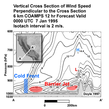
In this cross section, we see a strong maximum in mountain-parallel flow on the windward side of the barrier, signifying the development of a low-level barrier jet. Wind speed in the core approaches 30 m/s, or almost 60 knots! This low-level jet occurs 400 km or more ahead of the surface cold front, which lies just along the left edge of the cross section.
The strong along-mountain flow is well removed from the core of stronger winds that occur just ahead of the front at 900 hPa. Simulations without topography show that this low-level jet fails to develop without the presence of the mountain barrier.
Modification of the Prefrontal Wind Field » Case Example: 27 October 1999
Modification of the Prefrontal Wind Field » Case Example: 27 October 1999 » Introduction
Let's take a look at a 27 October 1999 case of a landfalling cyclone and associated frontal systems. We will examine the evolution of the mesoscale structure of the wind and precipitation fields along the coastal mountains. Some questions to consider include:
- What is the synoptic pattern that produces topographic effects?
- How does it evolve relative to the coastal topography?
- What mesoscale effects come into play as the front comes ashore?
Modification of the Prefrontal Wind Field » Case Example: 27 October 1999 » Synoptic Setting
Question 12
On the image below:
- Use the pen to mark where you would expect to find a strong flow interaction with topography.
When you have finished, select Done.
Compare your answer to the answer below.
The correct answer is Northern California. The sea-level pressure forecast shows the isobar pattern running parallel to the coast through Washington and most of Oregon throughout the loop. With geostrophic flow oriented parallel to the isobars, and subsequently parallel to the coast, there will be very little interaction between the flow and the topography in this region.
While the isobars remain parallel to the Washington coastline, they cross the coast at a high angle from southern Oregon southward to San Francisco Bay. Southwesterly flow just below mountaintop level will lead to the greatest topographic effects in this region. Furthermore, there is a strong low-level pressure gradient to the south of the cyclone center with southwest flow aloft, which is most likely characterized by warm advection along the coast of northern California. Consequently, the northern California coast has the potential for flow blocking and development of a barrier jet.
Modification of the Prefrontal Wind Field » Case Example: 27 October 1999 » How do forecast models handle the case of a landfalling front? The 40km Eta Model
Since complex mesoscale flow interactions with topography occur in association with landfalling fronts, it stands to reason that higher-resolution NWP models will simulate these interactions more realistically than coarser-resolution models. In order to gain better insight into the effects of model resolution in forecasting the effects of landfalling fronts, we will now examine a case from 27 October 1999 using coarse- and fine-resolution NWP models. The coarse model is the 40-km Eta, while the finer-resolution model is the 12-km MM5.
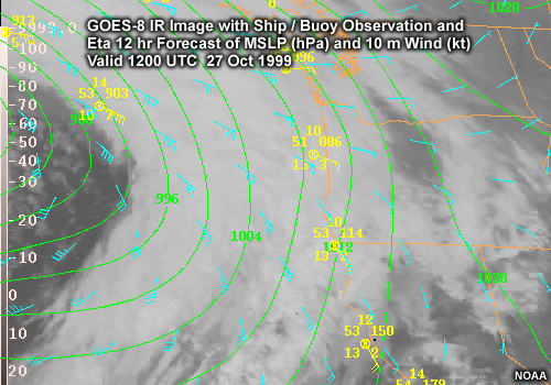
This image shows a GOES-IR satellite image overlaid with the 12-hour Eta forecast of sea level pressure, model winds, and buoy observations, valid at 1200 UTC on 27 October. With the front still well offshore, the model forecast winds compare favorably with the observed surface winds. The model-derived winds and buoy observations both show that the flow is deflected across isobars toward lower pressure. The cross-isobar winds probably reflect an ageostrophic response of the wind field as it encounters the coastal topography.
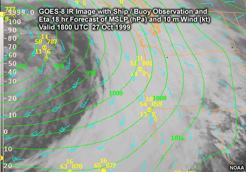
By 1800 UTC, the Eta model depicts the front approaching the Washington/Oregon coastline. Offshore of the northern California coast, we see southwest flow ahead of the front, but a distinct change to southerly and southeasterly flow along the coast. This change reflects the ageostrophic acceleration of winds along the coast, possibly due to flow blocking.
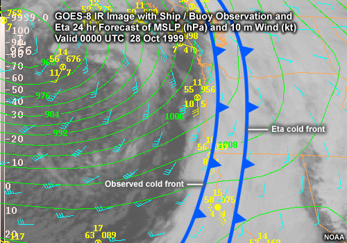
By 0000 UTC the observed front is pushing onshore, with the coastal buoys continuing to show coast-parallel flow. However, the Eta model was much faster at bringing the front onshore and shows it well inland over northern California at this time. The buoy observations along the northern California coast show 45-knot surface winds parallel to the coast suggesting a rather well-developed barrier jet.
Clearly, the coarse-resolution Eta model forecast is too fast on the frontal movement across the coast. This may occur because the model does not adequately handle the dynamic effects of topographic blocking that slow the front down as it approaches the coast and initiates development of the barrier jet. These limitations should be taken into account when using coarse resolution models, such as the 40-km Eta, to forecast landfalling fronts along the West Coast.
Modification of the Prefrontal Wind Field » Case Example: 27 October 1999 » What kind of coastal wind effects occur with this landfalling front in 12-km MM5 forecasts?
Question 13
Now let's examine a high-resolution simulation for the same event, using the 12-km MM5. This figure shows an 18-hour forecast of the low-level wind field and isotachs, along with ship and buoy observations, superimposed on a GOES IR image.
On the image below:
- Use the pen to mark the strongest wind.
When you have finished, select Done.
Compare your answer to the answer below.
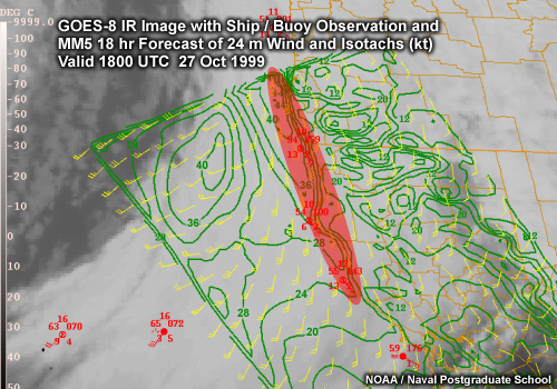
The isotachs show a relative maximum in the SSE flow right along the coast of northern California and southern Oregon. This relative maximum extends southward along the coast with stronger winds right along the coast and weaker winds further offshore. Further offshore the winds strengthen once again in advance of the frontal trough.
At this time, the front was strongly interacting with the northern California coast. The pattern of stronger winds along the coast, weak winds offshore, and strengthening near the front is common as fronts approach the continent. In this case, the effect is especially pronounced in the northern part of the model domain. It appears that the high-resolution mesoscale model does a reasonable job capturing the details of the topographic interaction that results in the development of a coastal barrier jet.
Modification of the Prefrontal Wind Field » Case Example: 27 October 1999 » Evolution of Thermal Structure and Along-Mountain Flow
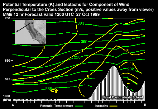
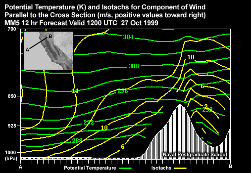
Now let's consider the dynamics that produce the topographic interaction and stronger winds right along the coast. First we examine cross sections and model soundings from the MM5 model simulation. The first set of cross sections shows potential temperature and isotachs for the wind component oriented perpendicular to the cross section (in other words, the coast-parallel flow). The cross sections run ENE-WSW, perpendicular to the California coastline.
We start with the 12-hour forecast, when the front is still well offshore. Note that the isentropes, which started out fairly horizontal when the front was much further to the west, now slope upward toward the mountains. This change in slope occurred because prefrontal warm advection depressed the isentropes offshore, while those near shore stayed relatively unchanged. Consequently, isentropes slope upward toward the coast. The result is a pocket of cooler air near the surface right next to the mountains and an increase in stratification over the top of this cool air, shown by the tighter packing of the isentropes. Given the implied horizontal thermal and pressure gradients across the coast, thermal wind balance requires that the prefrontal southerly wind should increase toward the surface. The isotachs in the model show this increase and produce a wind maximum along the coast, but there is no core structure resembling a barrier jet at this time.
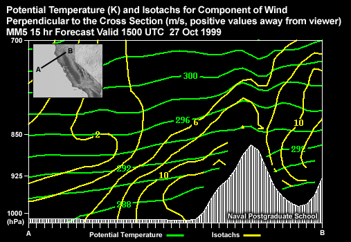
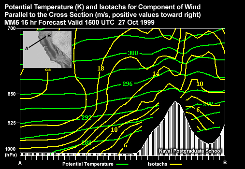
By 1500 UTC, the winds normal to the cross-section have strengthened considerably and there is a semblance of a barrier jet structure developing windward of the coastal range. There is still a gradual slope of isentropes downward offshore, consistent with thermal wind balance and the low-level wind maxima. This slope tends to steepen with time as the prefrontal warm air advection increases at low levels and the front moves closer to the coast.
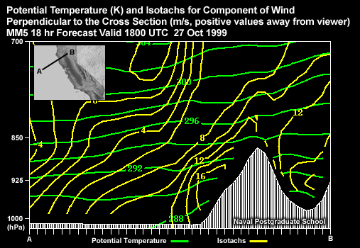
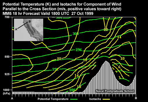
By 1800 UTC, the cross section shows a well-developed barrier jet, with the southerly wind component intensifying to greater than 16 m/s. Notice that the low-level stratification has not increased much over the coastal zone in this case, which limits its longevity. However, as the warm prefrontal air progresses closer to the coast, the slope of the 288K isentrope steepens, which amplifies the barrier jet wind speed.
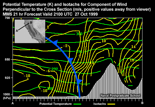
By 2100 UTC, the cold front lies just offshore. Cool temperatures behind the cold front result in a ridging of the isentropes with the slope of isentropic surfaces now reversed to slope downward toward the coast. Also note that the barrier jet has now been lifted toward the mountaintop level and the isentropes out ahead of the front have flattened.
Although the winds near the base of the mountains continue to be strong ahead of the front, they have weakened when compared with the previous time period. Recall that the isentropic slope was much greater at that time due to the trapping of the cooler air against the mountains.
Modification of the Prefrontal Wind Field » Case Example: 27 October 1999 » Cross-Mountain Flow Interaction with the Topography
Now let's examine MM5 model cross sections of the flow perpendicular to the coastal mountains for the same period to further illustrate how it interacts with the mountains.
At 1200 UTC the wind speed at around 950 hPa decreases from 14 m/s far offshore to 6 m/s near the coastal mountains. This speed decrease is most pronounced below mountaintop level, which is consistent with some blocking of the cross-mountain flow even when the front still lies far offshore.
Now we watch the cross-mountain flow evolve as the barrier jet develops. At 1500 UTC note that, in general, the cross-mountain flow increases as the front approaches the coast. However, flow near the base of the mountains remains fixed at about 6 m/s. Thus, the cross-mountain wind speeds show an increasing tendency to decelerate in the coastal region.
By 1800 UTC, when the barrier jet has become well developed, the cross-mountain flow decreases from 22 m/s offshore ahead of the front to less than 10 m/s along the coast in the barrier jet. This deceleration is consistent with flow blocking and the increasing slope of the isentropes in the coastal region.
Modification of the Prefrontal Wind Field » Case Example: 27 October 1999 » Determination of Blocking (1 of 3)
Is the prefrontal flow blocked? We can determine this by examination of the Froude number (Fr). Recall that Fr=U/(Nh), where U is the cross-mountain flow, N is the Brunt-Vaisala frequency, and h is the mountain height. When the Fr < 1, the flow tends to be blocked, while the winds tend to flow over the mountain barrier for Fr > 1.
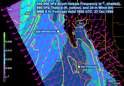
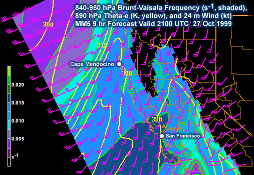
This figure shows a 6-hr MM5 forecast of equivalent potential temperature (theta-e), Brunt-Vaisala frequency (N), and 24-meter winds valid at 1800 UTC on 27 October. Recall that this is the time when a pronounced barrier jet was evident on the previous cross sections. In the northern part of the domain, we note the warm, moist theta-e ridge ahead of the approaching cold front, with cooler, drier air (lower theta-e) behind the front.
Question 14
For a point near Cape Mendocino, will the flow be blocked at this time? Use Froude Number Calculator. (Choose the best answer.)
The correct answer is a).
Please conintue watching the video above.
The Brunt-Vaisala frequency is relatively high ahead of the front (greater than 15 x 10-3), with significantly lower values behind the front (less than 10 x 10-3). Relatively undisturbed winds offshore look to be south-southwesterly at about 25 to 30 knots. With a mountain barrier height of approximately 1500 meters, the Froude number works out to less than one in the coastal region immediately ahead of the front. So it appears that the cross-barrier flow is blocked, at least near the base of the mountain.
Sidebar: Computation of the Froude number
If wind speed = 10 m/s, wind angle =
40°, N = 0.015 s-1, and h = 1500 m,
and Fr = U / (Nh)
Fr = 0.47
Now we will attempt to ascertain if the low-level flow will stay blocked as the front approaches the coastline and subsequently passes inland.
Modification of the Prefrontal Wind Field » Case Example: 27 October 1999 » Determination of Blocking (2 of 3)
At 2100 UTC, conditions have not changed much. The front is still offshore and the flow ahead of the front is still about 25-30 knots toward the coastal topography. The Brunt-Vaisala frequency remains high ahead of the front and drops off dramatically behind it. This suggests that the flow continues to be blocked to maintain the barrier jet along the coast.
Modification of the Prefrontal Wind Field » Case Example: 27 October 1999 » Determination of Blocking (3 of 3)
Question 15
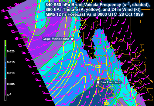
By 0000 UTC 28 October, the front appears to have passed inland in northern California. What is the Froude number now? Use Froude Number Calculator. Enter your response and select Done.
The Brunt-Vasala frequency drops off rapidly behind the front to a value of approximately 0.007. Meanwhile undisturbed winds offshore are about 20 knots at a high angle to the coast. Thus, the Froude number appears to have increased to about 1 along the northern California coast in response to weaker postfrontal winds and the lowered Brunt-Vaisala frequency associated with lower stability behind the front. Although the flow becomes unblocked, the low-level winds are still deflected northward along the coast, rather than westerly as we would expect behind the front. The persistence of southerly winds in the near coast environment results from 2 factors that combine to rotate isobars toward a coast-parallel direction:
- A large-scale pressure distribution still supporting southerly flow, and
- Weak windward ridging effects in the unblocked flow.
Modification of the Prefrontal Wind Field » Case Example: 27 October 1999 » Operational Determination of Stability
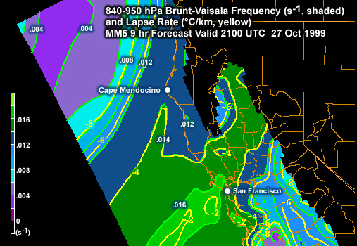
While the Brunt-Vaisala Frequency is a useful measure of atmospheric stability and a factor in the computation of the Froude number, it is not commonly used in an operational setting. A more common measure of stability is the atmospheric lapse rate. For example, we all know that the dry adiabatic lapse rate is about 9.8°C/km and that the lapse rate of the standard atmosphere in the U.S. is about 6.5°C/km. What might not be clear is that the Brunt-Vaisala Frequency and the lapse rate are closely related. This figure shows both the MM5 forecast of lapse rate and Brunt-Vaisala Frequency for 2100 UTC. Note that the yellow lapse rate contours closely mimic the color-filled Brunt-Vaisala Frequency contours. We can see that the least stable area in the northwest corner of the plot has a lapse rate exceeding 8°C/km and a Brunt-Vaisala Frequency less than 6 x 10⁻³ (0.006). In other words, as the lapse rate approaches 9.8°C/km, the Brunt-Vaisala Frequency approaches 0. Similarly, a lapse rate of 6.5°C/km roughly corresponds with a Brunt-Vaisala Frequency of 10 x 10-3 (0.010).
On this figure, note the sounding location near Cape Mendocino.
This animation of model soundings shows the evolution of the atmosphere just south of Cape Mendocino as the front makes landfall. Compare the relatively stable prefrontal environment to the much less stable postfrontal environment. The initial sounding in the sequence shows a very stable marine boundary layer capped by an inversion, while the last sounding displays a low-level lapse rate very close to dry adiabatic. Also note the pronounced wind shift with frontal passage, from more southerly to more westerly. These changes are typical of landfalling fronts and lead to the topographic interactions we just discussed.
Modification of the Prefrontal Wind Field » Case Example: 27 October 1999 » Conclusions
In conclusion, the interaction of landfalling fronts with coastal topography produces important modifications to coastal winds. The tendency of the coastal mountains to block the onshore advection of warm air results in low-level blocking and the development of a barrier jet along the coastal mountains. Strong differential warm advection that helps to increase stability with moderate onshore flow is highly favorable for flow blocking and a barrier jet. The angle that the front makes with the coast can be important in determining the degree to which flow blocking might occur.
Effects on the Postfrontal Wind Field
Effects on the Postfrontal Wind Field » Case Example: 14-16 March 2003
Effects on the Postfrontal Wind Field » Case Example: 14-16 March 2003 » Introduction
Now let's consider a different sort of event where the synoptic situation is similar, yet the wind field evolves in a different manner. In this case, while coastal topography exerts little effect on flow ahead of the front, it still contributes to a turning and acceleration of winds after frontal passage.
Effects on the Postfrontal Wind Field » Case Example: 14-16 March 2003 » Synoptic Setting
This animation shows IR satellite imagery and sea level pressure forecasts for a cyclone and landfalling front on 14-15 March 2003. The animation shows a well-developed cyclone tracking northeastward toward the coast of British Columbia from a position several hundred kilometers off the California/Oregon coast. A frontal cloud band trails to the southwest of the cyclone. The western edge of the frontal cloud band is sharply defined, and gives a good indication of the surface front location. It appears that the surface front first comes ashore near the California/Oregon border between 0600 and 0900 UTC on 15 March.
Question 16
In southern Oregon and Northern California, what is the orientation of the front with respect to the coastline? (Choose the best answer.)
The correct answer is a).
In the region near the California/Oregon border, the front is oriented nearly parallel to the coast, and stays that way as it makes landfall.
Effects on the Postfrontal Wind Field » Case Example: 14-16 March 2003 » Prefrontal Wind Response
The prefrontal winds in this case are rather strong (greater than 30 kt) and coast-parallel, similar to the case with blocked flow.
Question 17
This loop of east-west cross sections through the front shows isotachs and theta-e before and during landfall. What appears to be the most likely cause of the strong prefrontal winds? (Choose the best answer.)
The correct answer is b).
As this animation shows, the strong winds in this situation are easily explained as a well-defined prefrontal jet and are not due to the development of a barrier jet in blocked flow.
Effects on the Postfrontal Wind Field » Case Example: 14-16 March 2003 » Postfrontal coastal wind response
Question 18
This animation shows observed and model winds for the postfrontal environment after 0600 UTC. How would you characterize the wind field far offshore and close to shore? (Choose all that apply.)
The correct answers are a) and d).
Please continue watching the video above.
The winds are nearly geostrophic more than 200 km off the coast, but exhibit a more pronounced coast-parallel, southerly ageostrophic component near the coast. This is similar to what we observed in the prefrontal environment. However, in this case the wind speeds are considerably slower and occur in a postfrontal environment, which does not favor flow blocking.
Question 19
What happens to the mesoscale pressure field in northern California during and after landfall of the front? (Choose the best answer.)
The correct answer is b).
Please continue watching the video above.
Note the ridging in the pressure field along the coast in northern California and southern Oregon. While there were hints of ridging ahead of the front, the ridge becomes more established after the front passes inland. This ridging suggests that the flow is not blocked, with flow over the mountains producing a windward ridge after frontal passage. The mesoscale ridging results in a pressure gradient that is more perpendicular to the coast than the synoptic-scale pattern suggests.
Six hours later at 0000 UTC on 16 March, nearshore winds continue to parallel the coast and the southerly response extends even farther to the south, with prominent ridging in the sea-level pressure field near the coast and troughing inland of the coastal mountains. The synoptic and mesoscale pressure pattern has remained rather similar throughout the period, which allows the flow to adjust more geostrophically to the pressure distribution. This extended period of mesoscale ridging is particularly important. It allows time for the winds to respond to the mesoscale pressure distribution.
Effects on the Postfrontal Wind Field » Case Example: 14-16 March 2003 » Dynamics
Obviously, the evolution here is somewhat different than what we saw in the earlier case. In both instances, we observed the prefrontal winds to be strong and rather coast parallel. However, the prefrontal structure was different due to the differing orientation of the front relative to the coast. In this case, as the front moved onshore, the winds turned toward the coast for only a brief period, followed by a return to a southerly, coast-parallel direction. So what are the dynamics in this situation both ahead of and behind the front?
Effects on the Postfrontal Wind Field » Case Example: 14-16 March 2003 » Coast-Parallel Flow
Here we see an E-W cross section of the potential temperature and the wind speed perpendicular to the cross section for 0300 UTC, about 3 hours before the front made landfall. A prominent 40 m/s southerly jet occurs ahead of the front at 900 hPa and propagates along with it. As we saw previously, this prefrontal jet occurred even when the front was offshore and is due to the baroclinic structure of the front. Note that the cross section shows little of the isentropic rise toward the coast that we saw in the previous case when the flow was blocked. The synoptic-scale flow that occurs ahead of the front in this case is parallel to the coastal mountains so there is very little interaction with the topography.
By 1200 UTC, the front is past the coastal mountains as shown by the isentropes sloping downward to the east. There is a weak coastal jet near the coastal mountains with a peak southerly component of 10 kt. This feature appears locked to the topography. This weak barrier jet continues for the next 12 hours or so as noted previously.
Effects on the Postfrontal Wind Field » Case Example: 14-16 March 2003 » Cross-Coast Flow
Now consider the cross-barrier flow. The E-W cross-section above shows the potential temperature and cross-coast wind component at 0300 UTC, the same time that we observed the 40 m/s southerly jet. Note that the low-level cross-barrier flow has negative values in the vicinity of the coastal range, indicating offshore flow. Even though the stratification is probably sufficient to produce blocking, the prefrontal wind component is directed offshore and so it produces very little response.
As the front passes inland, the flow over the topography increases to about 6 m/s.
Effects on the Postfrontal Wind Field » Case Example: 14-16 March 2003 » Cross-Coast Flow Question
Question 20
This model sounding is located just offshore along the line of the cross section we just saw. How would you characterize the atmosphere in the lowest 150 hPa? (Choose the best answer.)
The correct answer is a).
In this case, the low levels are only weakly stratified. Note that the lapse rate in the lowest levels is very close to dry adiabatic. Consequently, the wind is able to move up and over the topographic barrier.
Effects on the Postfrontal Wind Field » Case Example: 14-16 March 2003 » Summary of Observations
The flow up over the mountains leads to the subtle windward ridging that we see in the cross section.
To summarize what we've observed in the cross sections:
1. In the prefrontal environment, we observe a 40 m/s, southerly prefrontal jet. Meanwhile,
near the base of the mountains, the component of flow parallel to the cross section is
directed offshore at about 8 knots.
2. In the postfrontal environment, we see a weak
jet-like feature in the component of wind oriented perpendicular to the cross section of
about 10 knots. The wind component parallel to the cross section shows flow of about 6 knots
up over the mountains. This cross-mountain flow is accomodated by weak stability in the post
frontal environment, and produces a windward ridge / lee trough response in the pressure
field.
Effects on the Postfrontal Wind Field » Case Example: 14-16 March 2003 » Comparison of Prefrontal and Postfrontal Cases
We have examined two cases that exhibited significantly different dynamic situations. In the first case, stably stratified cool air was trapped at low levels on the windward side of the coastal range. Although a windward pressure ridge developed, the flow was blocked by the topography and accelerated ageostrophically, resulting in the development of a strong southerly coast-parallel low-level jet. The blocked low-level flow resulted in slowing of the surface front as it approached the coast. In extreme cases, the front aloft continues toward the coast while the surface front stalls offshore. The resulting split front destabilizes the prefrontal environment, which enhances convective precipitation on the windward side of the coastal range.
In the second case, the prefrontal flow was coast parallel and resulted in minimal topographic interaction. Prefrontal winds were strong and coast parallel because the front had a strong low-level jet that was oriented along the coast due to the direction the front approached the coast. However, the postfrontal flow turned southerly and coast parallel except for a brief period of westerly flow. Only a very weak barrier jet developed in the postfrontal flow in this case but its existence was due to interaction of the cross-coast flow with the topography. The environment was less stable so that the flow was not blocked and was relatively unimpeded as it moved up and over the coastal range. Low-level windward pressure ridging and leeside pressure troughing resulted from upslope cooling and downslope warming as flow crossed the coastal mountains. The persistence of this pattern allows a 10-knot, along-coast flow to develop in association with the pressure gradient due to the windward ridging.
Effects on the Postfrontal Wind Field » Case Example: Yakutat Storm of 14 March 1979
Effects on the Postfrontal Wind Field » Case Example: Yakutat Storm of 14 March 1979 » Synoptic Setting
To illustrate the potential for postfrontal interaction let's briefly look at another case of a landfalling front. This case occurred on 14 March 1979 along the southeast Alaska coast and was described by Overland and Bond (1993). As we see in this animation, the landfalling front was aligned nearly parallel to the coast. Prefrontal winds were largely parallel to the coast, while postfrontal winds were more nearly perpendicular to the coast. Postfrontal flow up and over the mountains resulted in a pronounced windward ridge/lee trough.
Effects on the Postfrontal Wind Field » Case Example: Yakutat Storm of 14 March 1979 » Ageostrophic Wind Response
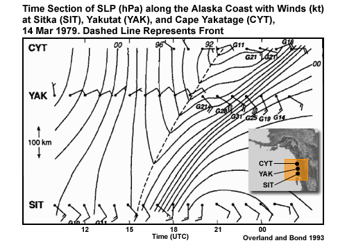
This figure shows a time series of wind observations at three surface sites along the coast. Frontal passage is denoted by the dashed line, as the front swings into the coast, then progresses northward. This plot shows very strong postfrontal winds in response to a strong pressure gradient that developed 3-6 hours after frontal passage. The largest pressure rises behind the front occurred where the cross-mountain flow was most favorable to produce windward ridging as it flowed up and over the coastal mountains. Adiabatic cooling of the postfrontal air rising up the slope produced a rapid pressure rise. This lead to development of a windward ridge and an associated strong ageostrophic wind response, with wind gusts to 31 m/s in YAK! This response was much stronger than that seen in the case we examined earlier along the California coast.
Effects on the Postfrontal Wind Field » Case Example: Yakutat Storm of 14 March 1979 » Conclusions
The previous cases illustrate the complexity of the dynamics associated with landfalling fronts along the West Coast. There can be many different dynamic scenarios, depending on the flow direction, stability, and a variety of other factors, which can alter the significance and subsequent impact of topographic effects. These various factors must be closely monitored in order to assess the potential impacts of topography on the mesoscale flow fields and also the precipitation patterns, which will be examined next, associated with these landfalling fronts.
Effects on the Postfrontal Wind Field » Questions
Effects on the Postfrontal Wind Field » Questions » Question
Question 21
A post frontal wind response is most likely to occur when the landfalling front is oriented _____. (Choose the best answer.)
The correct answer is a).
With the front oriented parallel to the coast, flow is similarly close to parallel to the coastal mountains. Consequently, there is little or no interaction between flow and topography.
Effects on the Postfrontal Wind Field » Questions » Question
Question 22
Use the pull-down menu to choose the best answer.
The correct answer is highlighted above.
As we have seen in soundings, the lapse rate increases with frontal passage, decreasing the stability.
Effects on the Postfrontal Wind Field » Questions » Question
Question 23
Use the pull-down menu to choose the best answer.
The correct answer is highlighted above.
Recall that the Froude number is U / (N * h), where N is the Brunt-Vaisala Frequency. When stability decreases, so does N. Thus, a decrease in stability results in an increase in the Froude number.
Effects on the Postfrontal Wind Field » Questions » Question
Question 24
When flow with a high Froude number encounters coastal mountains, what is the result? (Choose the best answer.)
The correct answer is b).
High Froude number flows can easily flow up and over mountain barriers.
Effects on the Postfrontal Wind Field » Questions » Question
Question 25
Unimpeded flow across the coastal mountains results in what phenomena? (Choose all that apply.)
The correct answers are a) and b).
Flow up over mountains produces cooling on the windward side and warming on the lee side of the barrier. This produces a windward ridge / lee trough in the pressure field. The windward ridge results in a pressure gradient more perpendicular to the coast. Given enough time, the low-level wind field will adjust to the pressure field and become more parallel to the coastal mountains.
Impacts on Fronts
Impacts on Fronts » Frontal Propagation: Horizontal Deformation
As we have seen, flow blocking and low-level barrier jets are rather common features in the prefrontal environment of landfalling fronts along mountainous coasts. However, more than just the wind field is affected by interaction of flow and coastal topography. Studies have shown that flow blocking ahead of landfalling fronts impedes frontal propagation so that the surface front tends to deform and become aligned with the topography. This conceptual animation illustrates how that occurs.
As the surface front approaches land, cool air is trapped along the coast and a southerly barrier jet develops. The trapped cool air impedes the landward progress of the surface front when it gets close to the coast. Meanwhile, parts of the front that are farther from the coast still progress landward until they encroach upon the trapped cool air, at which time their movement slows. With time, the surface front tends to deform and mirror the shape of the mountains.
Impacts on Fronts » Frontal Propagation: Development of a Split Front
This animation shows in cross section an extreme example of what can happen when a landfalling front encounters cool air trapped against the base of coastal mountains. The animation is based on a landfalling front in southern California described by Neiman et al. (2003).
While the surface front slows or stalls, the upper portion of the front is unimpeded by the blocking and continues to move toward the coast. Eventually, it shears off from and overruns the surface front. As a result, the cool, postfrontal air mass aloft flows over the warm, moist prefrontal air mass below it. This cool intrusion aloft destabilizes the near-coast environment, sometimes enhancing convective rainfall on the windward side of the coastal mountains. This destabilization combines with orographic lifting to produce very heavy rains and subsequent flooding in mountain valleys and rivers.
Eventually, a secondary frontal surge may sweep through. The merger of the primary and secondary fronts frequently leads to a narrow cold frontal rainband. Passage of the merged front typically scours out the trapped air near the surface. West winds behind the secondary front also increase the flow component normal to the mountains, combining with the lower postfrontal stability to increase the Froude number to values much greater than one. As a consequence, the flow at all levels is no longer blocked and passes freely over the coastal mountains.
Impacts on Mesoscale Precipitation Patterns
Impacts on Mesoscale Precipitation Patterns » Basic Orographic Precipitation Interaction
Precipitation fields are profoundly altered by the interaction of topography with landfalling fronts. Orographic effects modify the rainfall on both windward and leeward slopes.
As this animation clearly shows, precipitation associated with a landfalling front is concentrated on windward slopes, both along the coast and further inland in the Sierra Nevada.
At its most basic, the principal ingredients required for precipitation are moisture and lift. Upslope flow provides lift. Thus it follows that the greatest rainfall occurs where the flow is forced most strongly up a slope (given a similar moisture distribution). Conversely, lee slopes tend to experience descending flow, which inhibits precipitation.
Impacts on Mesoscale Precipitation Patterns » Low Resolution Model Representation of Precipitation
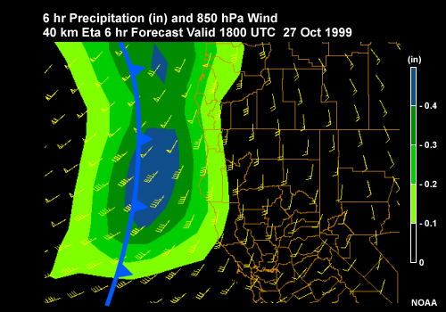
To illustrate how the dynamic interactions of the flow with topography can affect the mesoscale organization of precipitation, let's revisit the case of 27-28 October 1999. This figure shows the 6-hour Eta model forecast of the 850-hPa wind and precipitation for 1800 UTC on 27 October. Note the broad southerly flow ahead of the approaching front as well as the maximum in precipitation exceeding 0.4 inches offshore of the northern California coast, in the vicinity of the front.
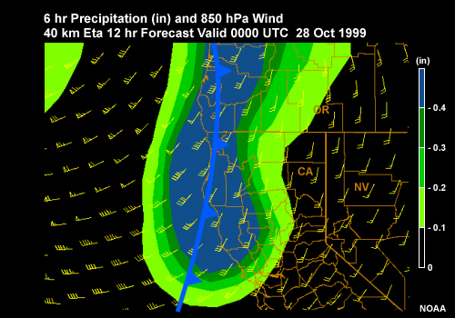
Six hours later, at 0000 UTC, the precipitation maximum approaches 0.7 inches in the vicinity of the front along the northern California coast. Also noteworthy are the strong southwest winds at 850 hPa, just ahead of the front. Given this flow and the topography, one might expect to see the largest precipitation amounts in southwest Oregon where the flow is strongest and oriented more across-mountain than further north or south. However, the Eta model appears to predict only coarse features and does not produce any mesoscale details of the precipitation distribution resulting from mesoscale interactions with topography.
Impacts on Mesoscale Precipitation Patterns » Mesoscale Model Precipitation Representation
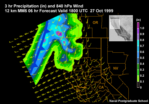
Now let's look at a higher resolution MM5 mesoscale model simulation of the 27-28 October 1999 case. The figures show 840-hPa wind and 3-hour accumulated precipitation. The 6-hour forecast valid 1800 UTC on February 27 progs a broad band of precipitation extending southwestward offshore in association with the front, similar to what was depicted in the coarser Eta model run. However, the MM5 model simulation depicts much greater mesoscale detail in the prefrontal precipitation field with maxima approaching or exceeding 1 inch along and immediately inland of the northern California/southern Oregon coastline. This detail reflects the ability of the higher resolution MM5 to more realistically simulate the topographic interactions that were altogether missed by the Eta model.
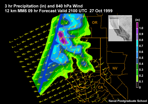
As the front moves onshore, the MM5 forecast valid at 2100 UTC continues to show mesoscale details of the orographic enhancement of precipitation on windward slopes.
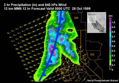
By 0000 UTC on 28 October, the MM5 simulation shows the front progressing inland over northern California, with a continuation of mesoscale orographic enhancement of precipitation now extending eastward to the mountains of the Sierra Nevada.
It is clear that higher-resolution model simulations are much better at depicting the mesoscale details of both the wind and precipitation fields associated with landfalling fronts.
Impacts on Mesoscale Precipitation Patterns » Blocking Effects on Precipitation
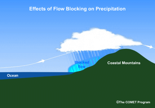
The orographic enhancement of precipitation along the coastal range is fairly easy to understand. For less stable situations where the flow across the mountains is relatively unimpeded, the maximum precipitation should be closely correlated with the area where maximum orographic lifting is occurring. However, if the environment is more stable, blocking of the flow can complicate the precipitation distribution. As this diagram shows, flow blocking may shift the orographic precipitation offshore, away from the windward slope. In this case, isentropes are shifted upward in the blocked region, resulting in the strongest isentropic lift occurring upstream of the topography.
Summary and Forecasting Considerations
In this module, we have considered dynamic topographic interactions that have a significant impact on the mesoscale structure of the wind and precipitation fields associated with landfalling fronts along mountainous coastlines. Now let's summarize by highlighting considerations relevant to forecasting these events.
The most significant issue regarding the forecasting of winds and precipitation characteristics for landfalling fronts in the coastal environment is the tendency of the flow to be blocked by the coastal topography. Flow blocking can enhance along-coast flow and alter the precipitation field.
In addition, mountain barriers can retard the progression of landfalling fronts. The degree to which there progress is slowed is dependent on the stability of the prefrontal environment. The greater the stability, the greater tendency for blocking and slowing of the frontal progression onshore.
Rainfall enhancement tends to be maximized along windward slopes where the cross-mountain flow is strongest. If the flow is blocked, the precipitation maximum may be shifted offshore, away from the windward slope. Under more extreme examples of flow blocking, the front may split, with the front aloft running ahead of the surface front. This may destabilize the environment leading to a convective enhancement of precipitation along windward slopes.
Mesoscale models capture topographic effects to some degree, depending on their resolution and accuracy in depicting the low level stability/stratification. In general, the higher the resolution, the more realistic the simulation. A more realistic representation of the topography allows models with sufficient resolution to produce flow blocking more readily in situations that may be marginally blocked in a low-resolution model. Low-resolution models will forecast fewer topographic effects. Thus they will turn the winds less along the coast and show little impact on frontal propagation.
Model forecasts are especially sensitive to changes in flow direction and stability.
Low-level stability is the most important factor, as it will determine whether the flow is blocked, which can significantly impact the mesoscale structure of the wind and precipitation fields.
Be aware of signatures such as that of a developing barrier jet in the model simulations and the observations. Model cross-sections of coast parallel flow fields may be helpful in diagnosing and forecasting the development of a barrier jet.
Empirical evidence indicates that the topographic impacts are most significant when the Froude number is near 1 and the wind direction is at about a 45° angle to the mountain barrier.
Bibliography
Braun, S.A., Rotunno, R., Klemp, J.B., 1999: Effects of Coastal Orography on Landfalling Cold Fronts. Part I: Dry, Inviscid Dynamics. J. Atmos. Sci., 56, 517-533.
Braun, S.A., Rotunno, R., Klemp, J.B., 1999: Effects of Coastal Orography on Landfalling Cold Fronts. Part II: Effects of Surface Friction. J. Atmos. Sci., 56, 3366-3384
Doyle, J.D., 1997: The Influence of Mesoscale Orography on a Coastal Jet and Rainband. Mon. Wea. Rev., 125, 1465-1488
Egger, J., and Hoinka K. P., 1992: Fronts and orography. Meteor. Atmos. Phys., 48, 3-36.
Kurz, M., 1990: The influence of the Alps on structure and behaviour of cold fronts over southern Germany. Meteor. Atmos. Phys., 43, 61-68.
Neiman, P.J., Persson, P.O.G., Ralph, F.M., Jorgensen, D.P., White, A.B., Kingsmill, D.E., 2004: Modification of Fronts and Precipitation by Coastal Blocking during an Intense Landfalling Winter Storm in Southern California: Observations during CALJET. Mon. Wea. Rev., 132, 242-273
O'Handley, C., and Bosart L.F., 1996: The impact of the Appalachian Mountains on cyclonic weather systems. Part I: A climatology. Mon. Wea. Rev., 124, 1353-1373.
Overland, J.E., Bond, N.A., 1993: The Influence of Coastal Orography: The Yakutat Storm. Mon. Wea. Rev., 121, 1388-1397
Overland, J.E., Bond, N.A., 1995: Observations and Scale Analysis of Coastal Wind Jets. Mon. Wea. Rev., 123, 2934-2941
Pierrehumbert, R.T., and Wyman B., 1985: Upstream effects of mesoscale mountains. J. Atmos. Sci., 42, 977-1003.
Schumacher, P.N., Knight D.J., and Bosart L.F., 1996: Frontal interaction with the Appalachian Mountains. Part I: A climatology. Mon. Wea. Rev., 124, 2453-2468.
Sinclair, M.R., Wratt D.S., Henderson R.D., and Gray W.R., 1997: Factors affecting the distribution and spillover of precipitation in the Southern Alps of New Zealand: A case study. J. Appl. Meteor., 36, 428-442.
Smolarkiewicz, P.K., and Rotunno R., 1990: Low Froude number flow past three-dimensional obstacles. Part II: Upwind flow reversal zone. J. Atmos. Sci., 47, 1498-1511.
Contributors
COMET Sponsors
- National Oceanic and Atmospheric Administration (NOAA)
- National Weather Service (NWS)
- Naval Meteorology and Oceanography Command (NMOC)
- Air Force Weather Agency (AFWA)
- National Environmental Satellite, Data, and Information Service (NESDIS)
- Environment Canada - Meteorological Service of Canada (MSC)
- Australian Bureau of Meteorology (BoM)
Project Contributors
Principal Science Advisors
- Dr. Wendell Nuss - Naval Postgraduate School
Project Lead/Instructional Design
- Dr. Alan Bol - UCAR/COMET
Project Co-lead/Project Meteorologist
- Dr. Greg Byrd - UCAR/COMET
Computer Graphics/Interface Design
- Steve Deyo - UCAR/COMET
- Heidi Godsil - UCAR/COMET
Multimedia Authoring
- Dan Riter - UCAR/COMET
Audio Editing/Production
- Seth Lamos - UCAR/COMET
Audio Narration
- Stephen St. James
COMET HTML Integration Team 2021
- Tim Alberta — Project Manager
- Dolores Kiessling — Project Lead
- Steve Deyo — Graphic Artist
- Ariana Kiessling — Web Developer
- Gary Pacheco — Lead Web Developer
- David Russi — Translations
- Tyler Winstead — Web Developer
COMET Staff, May 2006
Director
- Dr. Timothy Spangler
Deputy Director
- Dr. Joe Lamos
Business Manager/Supervisor of Administration
- Elizabeth Lessard
Administration
- Lorrie Alberta
- Linda Korsgaard
- Bonnie Slagel
Graphics/Media Production
- Steve Deyo
- Heidi Godsil
- Seth Lamos
Hardware/Software Support and Programming
- Tim Alberta (IT Manager)
- James Hamm
- Karl Hanzel
- Ken Kim
- Mark Mulholland
- Dan Riter
- Carl Whitehurst
- Malte Winkler (student)
Instructional Design
- Patrick Parrish (Production Manager)
- Dr. Alan Bol
- Lon Goldstein
- Dr. Vickie Johnson
- Bruce Muller
- Dwight Owens
- Dr. Sherwood Wang
Meteorologists
- Dr. Greg Byrd (Project Cluster Manager)
- Wendy Schreiber-Abshire (Project Cluster Manager)
- Dr. William Bua
- Patrick Dills
- Tom Dulong
- Kevin Fuell
- Dr. Stephen Jascourt
- Matthew Kelsch
- Dolores Kiessling
- Dr. Arlene Laing
- Elizabeth Mulvihill Page
- Dr. Doug Wesley
Software Testing/Quality Assurance
- Michael Smith (Coordinator)
Spanish Translations
- David Russi
NOAA/National Weather Service - Forecast Decision Training Branch
- Anthony Mostek (NWS COMET Branch Chief [acting] and Satellite Training Leader)
- Dr. Richard Koehler (Hydrology Training Lead)
- Brian Motta (IFPS Training)
- Dr. Robert Rozumalski (SOO Science and Training Resource [SOO/STRC] Coordinator)
- Shannon White (AWIPS Training)
Meteorological Service of Canada Visiting Meteorologists
- Phil Chadwick
- James Cummine