Scenario
Scenario » Midwatch
Early morning, 25 June 2003 (0200 UTC, 0600 LT)
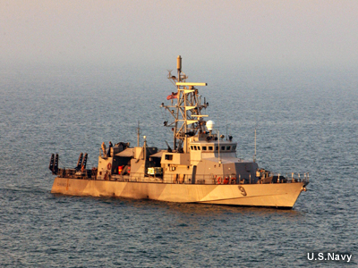
I was working the midwatch in Bahrain when we got a call from several Cyclone-class Coastal Patrol (PC) boats.
Scenario » Arabian Passage
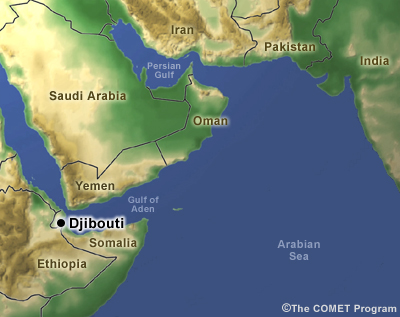
They wanted a sea-state forecast for a transit along the Oman coast into the Persian Gulf. The PCs had refueled in Djibouti and left yesterday. They recently exited the Gulf of Aden. From past experience, they were concerned about waves raised by the Somali Jet.
Scenario » Current Forecast
[ship at 15N 52E]
I pulled up the current forecast. Our sea-state forecast for this afternoon calls for 8-10 foot seas along the coast with 15-18 foot seas farther offshore in the core of the Somali Jet. So far, so good. The PCs have a 12-foot sea-state operating limit.
How about the synoptic picture? The 0000 UTC global GFS run was just becoming available, so I checked the latest forecast. Synoptic conditions aren't really expected to change much over the next day or so.
Scenario » Somali Jet
As for low-level winds, the analysis shows southwesterly winds across the northern Arabian Sea and the Gulf of Aden. The low-level barbs suggest that the Somali Jet will graze the coast of Oman.
However, winds are forecast to shift to a more westerly direction, with the core of the Somali Jet nearly 500 kilometers off the coast of Oman. That ought to keep the higher wave heights well offshore. This is a pretty typical pattern for this time of year and our sea-state forecasts for the AOR reflect it.
The model shows winds in the Gulf of Aden and along the Oman coast strengthening slightly over the next few hours. But that shouldn't be a problem and should not really build the seas.
I expect that the PCs will be well within their 12-foot sea-state operating limit, as long as they stay close to shore.
Scenario » COAMPS
Just to be safe, I checked the COAMPS forecast. The PCs are close to the edge of the model domain. But at least we can see the Oman coast; that's where any trouble will be.
The COAMPS forecast shows more variation, but overall it looks a lot like the GFS. I notice that it tightens up the pressure gradient along the coast and moves the higher winds closer to shore, especially near Ra's Mirbat. On the other hand, COAMPS shows decreasing winds through the next few hours. Either way, the winds aren't any higher than those progged by the GFS, so if the PCs can stay close to shore they should be OK.
Scenario » Late Afternoon, 25 June (1300 UTC, 1700 LT): Big Wind
[ship at 16N 55E]
After a rest, I'm back at my desk. In late afternoon I get word from the Coastal Patrols. They're reporting 35-knot winds as they approach the Ra's Mirbat. Seas are building with wave heights approaching 10 feet. They're wondering if conditions are still looking good to proceed. I pull up the latest obs. They don't really help. There's only a half dozen ship obs, and they're mostly farther offshore. What about the satellite winds?
I grab the latest scatterometer winds. It's not perfect, only a once-a-day peek that occurs first thing in the morning, so the winds could have strengthened. Still, I can see that the PCs are headed into the area with the strongest winds. Not good, and I still don't know what's going to happen. What can the models tell me?
Scenario » Double-Check
The latest COAMPS run is just coming out. The analysis still looks fine, although the wind forecast might be a little low in the model for the PCs' location. With so few observations going into the analysis, it's easy for the forecast to lag behind. Nonetheless, winds and swell should decrease to the east along the Oman coast in the next few hours.
Scenario » Trouble (1800 UTC, 2200 LT)
Yikes! I just got off the horn with the PCs. They're getting beat up out there with waves of 12-15 feet. Winds are still running 30 knots. What's going on? The captain was not at all happy when we talked and wants to know when they'll be out of this stuff.
Scenario » Almost Busted

It looks like a coastal jet has formed along the mountainous coastline of Oman. The jet is maintaining the strong winds exiting the Gulf of Aden. The global model hints at this, but it doesn't really keep things that strong. COAMPS has a better depiction of the jet, but also shows weaker winds.
Fortunately, both the GFS and COAMPS show that the coastal jet should diminish farther to the east. The seas should subside as well, particularly as the PCs turn the corner and head north out of the line of wave propagation.
I get on the horn and and tell the PCs to proceed east and things will improve! I can tell they are skeptical, but they stay on course. Later I hear that the coastal jet persisted throughout the night with winds in excess of 30 knots for at least 300 nautical miles.
Description of Large-Scale Features
Description of Large-Scale Features » Introduction
Low-level coastal jets occur along some coastlines due to the presence of a low-level baroclinic structure. These winds may exceed 35 knots, leading to high waves. Thus, coastal jets can significantly impact marine interests along the coast and immediately offshore. Coastal jets also lead to significant low-level vertical wind shear, thus presenting a hazard to aviation in the coastal zone.
Description of Large-Scale Features » Observations
So what exactly does a coastal jet look like? This example comes from California in August of 1999. We will use this case to illustrate the features of coastal jets throughout the module. This loop shows surface winds for a 24-hour period.
Question 1
Use the pull-down menu to choose the best answer.
The correct answers are highlighted above.
Please continue watching the video above.
Wind speeds are generally higher offshore than over land, and this difference persists throughout the day. On this particular day, land stations show 5-10 knot winds while coastal buoys have winds of 15-25 knots depending upon where along the California coast we look. There is little diurnal variation in offshore winds.
Description of Large-Scale Features » Sea Level Pressure

Without a doubt, one difference between the surface winds over land and those over the water is the difference in friction between land and water. Although lower friction offshore contributes to higher windspeeds, a more fundamental difference in the winds is found in the pressure field. This plot shows sea level pressure over the California coast during a coastal jet event. Note that the pressure distribution is distorted by the reduction to sea level for higher terrain. This distortion generates complex details in mountainous regions, particularly over the Sierra Nevada on the eastern edge of the plot.
Question 2
How does the pressure gradient change as one approaches the coast from offshore? Choose the best answer.
The correct answer is b.
Please continue watching the video above.
The pressure gradient increases as one approaches the coast. While there are variations up and down the coast, the maximum pressure gradient typically occurs at the coast and decreases both landward and seaward of this boundary.
Description of Large-Scale Features » Marine Boundary Layer
The factors that contribute to the strong cross-coast pressure gradient are most evident in a cross section of the structure across the coast.
Question 3
How would you characterize the marine boundary layer in this figure? Choose the best answer.
The correct answer is a.
Please continue watching the video above.
A cool, well-mixed marine boundary layer lies over the ocean, with few isentropes near the surface. This marine boundary layer is capped by an inversion, with tightly packed isentropes. The inversion slopes upward to the west, indicating a deepening marine layer with increasing distance offshore. This increase in depth is due to a combination of weakening large-scale subsidence farther west and generally warmer sea surface temperatures well offshore.
Question 4
What causes the near-vertical isentropes near shore? Choose the best answer.
The correct answer is b.
Please continue watching the video above.
The near-vertical isentropes seen near the coast result from the juxtaposition of the cool marine boundary layer with warmer air over the strongly-heated land surface.
Description of Large-Scale Features » Jet Structure
The sloping isentropes marking the top of the marine boundary layer comprise a baroclinic structure. This baroclinic structure leads to the strongest cross-coast pressure gradient at the surface, near the coast. For reasons we will discuss later, this structure yields the jet seen in this figure, the so-called California coastal jet.
Definition of Baroclinic: In a baroclinic state, isentropic surfaces are inclined to surfaces of constant pressure.
Question 5
Use the pull-down menu to choose the best answer.
How would you characterize the coastal jet?
The correct answers are highlighted above.
Please continue watching the video above.
As seen here, the jet core may be as narrow as 20 to 40 kilometers wide. The wind maximizes above the ground, near the base of the inversion, because friction retards the wind closer to the surface.
In a baroclinic state, isentropic surfaces are inclined to surfaces of constant pressure.
Description of Large-Scale Features » Coastal Mountains
The thermal structure described previously plays the dominant role in determining the presence of the coastal jet; however, topographic effects may also contribute to its intensity.
Question 6
What role do you expect topography to play in the development of coastal jets? Choose the best answer.
The correct answer is b.
Please continue watching the video above.
>Given the daily heating of the land surface onshore and the frictional slowing of surface winds over the ocean, one would expect at least a small component of non-geostrophic, onshore flow from high to low pressure. However, due to the presence of a strong low-level inversion, the coastal mountains tend to block this sea breeze component of the flow. Subsequently, this non-geostrophic component of the flow turns down the coast towards lower pressure. In California lower pressure typically lies to the south, so the non-geostrophic flow acts to increase the magnitude of the coastal northerly flow. Thus, coastal mountains help keep the flow oriented parallel to the coastline and suppress most of the sea breeze component that might develop. Suppression of the cool sea breeze helps to maintain the strong temperature and pressure gradient across the coast.
To learn more about how topography blocks flow, see the foundation module: Flow Interaction with Topography.
Description of Large-Scale Features » Summary
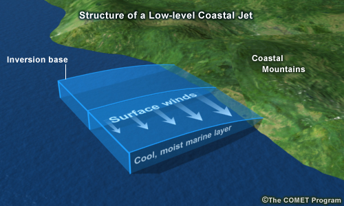
This figure summarizes the relationship between the low-level structure and the coastal jet. Because the inversion capping the marine boundary layer slopes downward toward the coast, the low-level temperature gradient reaches a maximum there. As a result, the sea level pressure gradient also reaches a maximum near the coast. Consequently, the low-level wind increases, leading to a coastal jet.
Thermal Gradients
Thermal Gradients » Thermal Wind
Thermal Gradients » Thermal Wind » Global SLP and Wind
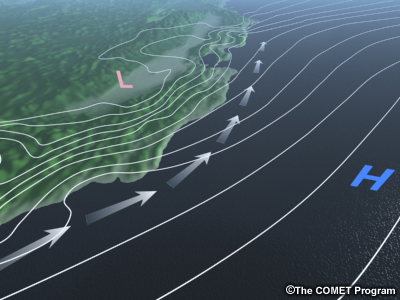
The large-scale conditions conducive to development of a coastal jet start with persistent synoptic flow oriented parallel to the coast. This animation shows composite charts of sea level pressure and surface winds. Note the subtropical high pressure systems located over the world's oceans. Anticyclonic circulation around these high pressure centers typically provide the synoptic flow that preconditions a coastal jet. Furthermore, we have seen that coastal jets develop when a well-developed, cool marine boundary layer forms that is capped by a strong inversion. Subsidence beneath a subtropical high pressure center, combined with a cool sea surface temperature leads to an inversion over the marine boundary layer. With time, the boundary layer cools and becomes well-mixed, which strengthens the capping inversion. Due to warmer temperatures over land, the inversion slopes down to the coast. This leads to a baroclinic structure that results in an acceleration of low-level flow near the coast.
Using these conditions, we can examine the climatologies of sea level pressure, surface winds, and sea surface temperatures to predict areas that are prone to coastal jets.
Question 7
Use the pull-down menu to choose the best answer.
The correct answers are highlighted above.
Pressure gradients and wind speeds are typically higher along the west coasts of continents.
Question 8
Use the pull-down menu to choose the best answer.
When would you expect coastal jets to occur at each of these locations?
The correct answers are highlighted above.
Coastal jets typically form in the warm months of the year, when temperature gradients, and thus pressure gradients, are greatest.
Thermal Gradients » Thermal Wind » Synoptic Patterns
Now, let’s look at the synoptic setting along the West Coast of the Unites States. The California coastal jet is associated with the larger-scale baroclinic structure of the atmosphere over the region during the summer. This becomes evident when we consider climatological analyses at 500 hPa, 850 hPa, and the surface.
Question 9
What is the main feature over the West Coast at 500 hPa? Choose the best answer.
The correct answer is d.
Please continue watching the video above.
At 500 hPa, a weak trough occurs off the West Coast and produces southwesterly flow aloft at about 20 knots.
Question 10
In this composite chart of 850-hPa heights, the strongest gradient occurs at which location? Choose the best answer.
The correct answer is c.
Please continue watching the video above.
The 850 hPa heights reveal high pressure offshore and a thermal low over Nevada. The pressure gradient reaches a maximum several hundred kilometers offshore. Near the coast, the height gradient at 850 mb yields only weak northwesterly flow at that level.
Question 11
What features are evident in this composite chart of sea level pressure? Choose all that apply.
The correct answers are b, c, and e.
Please continue watching the video above.
The thermally-induced surface low over the interior Southwest, combined with the subtropical high over the Pacific, results in a pronounced west-to-east pressure gradient that reaches a maximum near the coast. This results in persistent northwesterly winds at the surface of about 15-25 knots.
Thermal Gradients » Thermal Wind » Thickness and Wind
In the preceding pages, we established that a thermal gradient exists across the coast, and we have looked at the synoptic climatology associated with coastal jets. How do these conditions result in a low-level coastal jet?
Recall that the vertical distance or thickness between pressure surfaces is directly related to the mean temperature in the vertical layer.
Therefore, the strong horizontal temperature gradient at the surface is associated with a strong horizontal pressure gradient force, labeled PGF, from high pressure over the cold ocean to low pressure over the warm land. This is reflected by the steep slope of the 1000-hPa pressure surface.
As we move upward to 850 hPa, cooler temperatures over cold water result in a lesser thickness over the ocean, while warmer temperatures over land lead to a greater thickness onshore. Combined, the lesser thickness over the ocean and the greater thickness over land result in a more gentle slope for the 850-hPa surface than for the 1000-hPa surface.
Continuing upward to 500 hPa, the lesser thickness of the atmosphere over the ocean and the greater thickness of the atmosphere over land result in a reversal of slope. Consequently, the 500-hPa surface slopes down toward the ocean. This is the origin of the 500-hPa trough offshore that we previously observed in the 500-hPa climatology.
If the pressure gradient force and the Coriolis force are in geostrophic balance, then the magnitude of the geostrophic wind is directly proportional to the magnitude of the pressure gradient force and Coriolis force. Since the pressure gradient force is maximized at the surface near the coast, it stands to reason that the strongest winds should be observed near the surface. Due to friction effects, the observed wind maximum is typically a few hundred meters or so above the surface. The smaller pressure gradient at 850 hPa results in lighter winds at that level. Winds at 500 hPa reverse direction in response to the reversal in horizontal pressure gradient between 850 and 500 hPa. In California, this results in 500-hPa winds with a southerly component.
The coastal jet owes its basic existence to the persistence of the baroclinic structure at low levels, as described in the previous section. The detailed structure of the marine inversion becomes key in defining the jet structure: the slope of the strong inversion dominates in determining the thickness between the layers. Putting the two layers (surface-to-850 hPa and 850-to-500 hPa) back-to-back, it is evident that there is a thermal gradient aloft that turns the wind down coast. However, it is really the low-level thermal gradient that transforms this flow into a jet, and this low-level thermal structure is definitely a coastal effect.
Thermal Gradients » Thermal Wind » Case Example
This cross section from our California case illustrates the previous point. At low levels, isentropes slope down toward land, while at 500 hPa, isentropes slope in the opposite direction, down toward the ocean.
Thermal Gradients » Coastal Jet versus Sea Breeze Circulations
Thermal Gradients » Coastal Jet versus Sea Breeze Circulations » Diurnal Cycles
Along many coastlines throughout the world, a cool marine boundary layer coupled with warm air over land yields a strong sea breeze. At night, the land cools and the thermal gradient reverses, resulting in a land breeze. In the case of the coastal jet, the land/sea breeze plays only a minor role. Why is that?
Question 12
Use the pull-down menu to choose the best answer.
The correct answers are highlighted above.
Please continue watching the video above.
For both coastal-jet and sea-breeze circulations, the land warms and cools with a diurnal rhythm. However, in the case of the coastal jet, the sea surface temperature remains cooler than land through both day and night. This keeps low-level air temperatures cooler in the marine boundary layer than those over land. With enough time, the wind over the ocean approaches geostrophic equilibrium, flowing nearly parallel to isobars.
To learn more about sea breezes, see the foundation module: Thermally-forced Circulation I: Sea Breezes.
Thermal Gradients » Coastal Jet versus Sea Breeze Circulations » Exercise
These plots show surface temperatures during daytime and nighttime for two different coastal locations.
Question 13
Use the pull-down menu to choose the best answer.
The correct answers are highlighted above.
Please continue watching the video above.
>Location 1 (left-side image) occurs along the coast of southwest Africa. Note the cold ocean temperatures near shore with the high temperatures inland. This condition persists through a complete diurnal cycle. Consequently, a coastal jet results.
Location 2 (right-side image) occurs along the west coast of India. Note that while there is a strong thermal gradient along the coast, the high temperatures during daylight hours occur along the coastal plain, resulting in a sea breeze. At night the temperature gradient reverses and we see a land breeze. A coastal jet does not develop.
Thermal Gradients » Cold Sea Surface Temperatures (SSTs)
Thermal Gradients » Cold Sea Surface Temperatures (SSTs) » Cold Ocean Currents
What keeps the ocean cooler than land so that a coastal jet may develop? Cool sea surface temperatures have two origins: cold ocean currents and coastal upwelling.
Question 14

As this plot shows, many coastlines around the world are bathed by cold ocean currents. How would you characterize them?
Use the pull-down menu to choose the best answer.
The correct answers are highlighted above.
Please continue watching the video above.
Due to the nature of ocean circulations, cold ocean currents typically originate at high latitudes and lie along the west coasts of continents. Such cold currents include the California Current along the west coast of North America, the Peru Current along the west coast of South America, and the Benguela Current along the coast of southwest Africa.
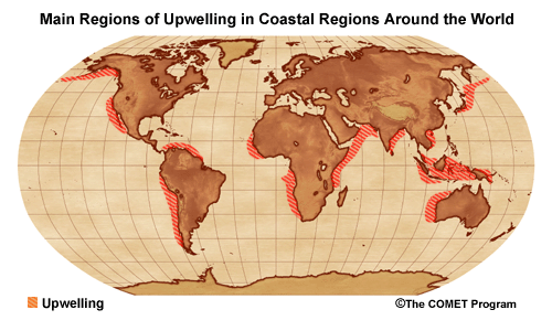
Thermal Gradients » Cold Sea Surface Temperatures (SSTs) » Coastal Upwelling
When winds blow with persistence over an ocean surface, the Coriolis force acts to move surface water at an angle to the wind direction: to the right in the northern hemisphere and to the left in the southern hemisphere. When winds push water offshore, cold water rises from beneath to replace it. This upwelling substantially reduces sea surface temperatures, which in turn reduces temperatures in the marine boundary layer.
In many cases, coastal upwelling further cools a cold ocean current. For example, persistent southerly flow along the coast of southwest Africa in the warm season causes coastal upwelling that further cools the cold water of the Benguela current.
Question 15
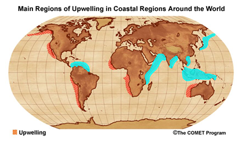
This map shows upwelling zones. Looking at this map, can you identify an area where upwelling occurs, but where ocean currents are warm, not cold?
On the image below:
- Use the blue pen to circle an area.
When you have finished, select Done.
Compare your answer to the graphic below.
Please continue watching the video above.
[Answer: anywhere around the Indian Ocean, Vietnam, Indonesia]
Coastal upwelling typically occurs in association with cold ocean currents. Thus, we see upwelling zones on the west coasts of most continents, such as North and South America, Africa, and Australia. In other cases, coast-parallel winds occur far from cold ocean currents. Such is the case with the Somali Jet, where warm southwesterly monsoon winds induce upwelling along the coasts of Somalia and Oman.
In most cases, the synoptic flow that preconditions formation of a coastal jet also promotes coastal upwelling. In turn, the upwelling cools the marine boundary layer, which increases the thermal gradient across the coast. The stronger thermal gradient leads to stronger winds, which promote even more upwelling. This positive feedback may sustain coastal jets for long periods.
Thermal Gradients » Cold Sea Surface Temperatures (SSTs) » Satellite Detection of SSTs

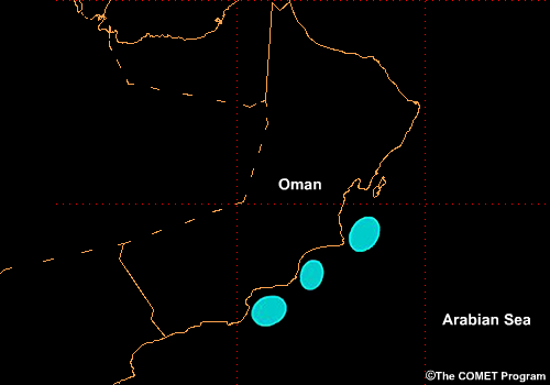
This plot shows satellite-derived sea surface temperatures for the scenario case that started this module. You can clearly see cooler water resulting from upwelling along the coast of Oman. Information like this is available in real time and gets incorporated into NWP models.
Along-Coast Variations
Along-Coast Variations » Variations in Wind Speed
An important aspect of coastal jets is their along-coast variability, which influences the distribution of clouds, winds, waves, and upwelling. This model simulation off the California coast depicts this along-coast variation.
Question 16
Where are the highest wind speeds located? Choose the best answer.
The correct answer is b.
Please continue watching the video above.
Maximum wind speeds generally occur downwind of coastal points and capes, such as Cape Mendocino and Point Sur, where the orientation of the coastline and coastal mountains changes substantially. The thermal gradient argument for the origin of coastal jets does not obviously explain this along-coast variability.
Along-Coast Variations » Wind Speed and Sea Level Pressure
These two figures show detailed observations of sea level pressure and wind south of Point Arena on the coast of Northern California.
Question 17
In the figure, do the highest wind speeds correlate with regions of high or low sea level pressure? Choose the best answer.
The correct answer is b.
Please continue watching the video above.
Note that the highest wind speeds coincide with the lowest sea level pressures. Lower pressures reflect a thinner marine boundary layer, while higher pressures reflect a thicker marine boundary layer. Thus higher wind speeds are associated with a thinner marine boundary layer and vice versa.
Along-Coast Variations » Hydraulics
So, what drives the thinning of the marine boundary layer and the acceleration of the flow? We can explain this phenomenon through hydraulic considerations, analogous to flow through a pipe.
As the flow passes a point or cape, it effectively moves offshore, opening a void between the flow and the coast. When this occurs, the flow reacts by spreading laterally to fill that void. We refer to this spreading as an expansion fan. As the flow spreads laterally, the marine boundary layer thins. The flow must now squeeze through a thinner boundary layer, that is essentially a smaller pipe. Consequently, the flow speeds up.
Conversely, as the flow approaches a point or cape, it effectively piles into a wall as it is blocked by the terrain. In response, the marine boundary layer abruptly thickens in what is termed a hydraulic jump. At this hydraulic jump, the pipe becomes larger and the flow slows down.
Along-Coast Variations » Defining the "Pipe"
The hydraulic analogy only works if the flow can be constrained to a pipe. This figure shows a mountainous coastline with a strong inversion at the top of the marine boundary layer. Thus, we can see that the flow is constrained at its base by the ocean surface and its top by the inversion. On the coastal side, we know that the inversion slopes steeply down toward the coast. With the base of the inversion below mountaintop level, the coastal mountains essentially act as a wall. The seaward side of the flow is constrained by a large-scale pressure gradient directed onshore to prevent flow away from the coastal channel. These conditions give us our "pipe."
Forecast Considerations
Forecast Considerations » Synoptic Considerations
Forecast Considerations » Synoptic Considerations » Introduction
Now that we've explored the nature of coastal jets, let's turn our attention to forecast considerations. In this section, we will reexamine the case that started this module. In that case, a coastal jet along the Oman coast hampered the passage of a group of Coastal Patrol boats in transit from Djibouti to the Persian Gulf.
Forecast Considerations » Synoptic Considerations » MSLP
The basic structure that supports a coastal jet is well depicted by synoptic scale numerical models. This loop shows the GFS forecast of sea level pressure over the Arabian Sea through 48 hours.
Question 18
Which of these statements best describe the pressure field along the Oman coast? Choose all that apply.
Please continue watching the video above.
These plots show persistent low pressure inland, with higher pressure offshore. The cross-coast pressure gradient increases during daytime in response to heating of land areas.
Forecast Considerations » Synoptic Considerations » Synoptic-Scale Winds
This plot shows the Somali Jet that results from the synoptic conditions depicted on the previous charts. This broad, large-scale low-level jet is the primary structure that is necessary before mesoscale coastal effects become important. Notice that along the Oman coast, the wind strengthens in the first 12 hours, but then stays remarkably constant through 48 hours, showing little diurnal variation.
Forecast Considerations » Synoptic Considerations » Marine Boundary Layer
Diurnal modulation of the cross-coast thermal gradient is expected due to the inland heating and lack of temperature change over the ocean. This contributes to some modulation of the coastal jet, but the background cross-coast pressure gradient tends to remain strong at all hours of the day. The cool MBL is of sufficient depth (up to 1000 m) to maintain a thermal gradient across the coast even with surface nocturnal cooling at night. This loop of forecast cross sections from Oman clearly shows a persistent cool marine boundary layer off the coast through 24 hours.
Forecast Considerations » Synoptic Considerations » 850-hPa Flow - Oman
Question 19
Use the pull-down menu to choose the best answer.
The correct answers are highlighted above.
There is evidence that the broad, low-level jet tends to hug the coast more effectively when the 850-hPa geostrophic flow is directed slightly offshore, as depicted in this plot from the Oman case. This seems to help establish and maintain an along-shore pressure gradient at the surface that causes the winds to accelerate along the coast. This is particularly true where the low-level flow tends to be blocked by coastal mountains, forcing the flow to be coast parallel, down the pressure gradient.
Forecast Considerations » Synoptic Considerations » 850-hPa Flow - California
The 850-hPa height analysis can often be used to identify a ridge axis that cuts across the coastline, as shown in this figure from California. To the north of this ridge axis, no coastal jet occurs. To the south of the ridge axis, the offshore 850-hPa geostrophic flow occurs and a coastal jet becomes very well established.
Forecast Considerations » Mesoscale Considerations
Forecast Considerations » Mesoscale Considerations » Wind Speed Variations
Along-coast variations in the coastal jet wind speeds are an important aspect to forecast.
Question 20
On the image below:
- Use the blue pen to highlight the location where you expect the highest wind speeds
When you have finished, select Done.
Compare your answer to the answer below.
Please continue watching the video above.
The regions of highest winds occur just downwind of coastal topographic headlands and points where the coast tends to turn away from the flow direction. This effect can be enhanced by mesoscale effects that lead to mesoscale regions of reduced pressure along the coast. For example, patchy fog dissipation and adiabatic warming of downslope winds can lead to small-scale variations in surface temperature, which will drop sea level pressure locally.
Numerical weather forecasts from mesoscale models such as the MM5 or COAMPS seem to produce mesoscale features in the wind field with ease. In fact, this COAMPS analysis for the Oman case portrays the primary features quite realistically. This suggests that if the MBL depth changes can be captured, then the model will produce realistic expansion fan type features.
Forecast Considerations » Mesoscale Considerations » Model Resolution: California
Resolution and physics appear to strongly affect a model's skill at depicting coastal jets. In this example from California, the 15-km MM5 keeps the coastal jet close to shore and accelerates winds to greater than 32 knots at the surface. On the other hand, the Eta model with 32-km resolution depicts a weaker jet located farther offshore with winds to 25 knots or so. The Eta subsequently fails to depict the fine-scale variations in wind speed induced by coastal capes and points.
Forecast Considerations » Mesoscale Considerations » Model Resolution: Oman
Depending on the model physics, some current global models appear able to capture some of the mesoscale complexity of coastal jets. Compare the analysis for the 18-km COAMPS with the 12-hour forecast for the global GFS. While COAMPS places high winds closer to shore, both COAMPS and GFS depict wind maxima downwind of points and capes. Maximum wind speeds are actually a bit higher in the GFS forecast. Thus it appears that forecast skill for different models depends on more than just resolution. It also depends on the model physics.
Forecast Considerations » Satellite Detection of Coastal Jets
Forecast Considerations » Satellite Detection of Coastal Jets » Scatterometer Winds
In the absence of a dense network of surface ship and buoy observations, newly-available products derived from polar-orbiting satellites may provide mesoscale details of the surface wind field. Satellite-derived data is especially important in data sparse regions overseas. This figure shows a QuikSCAT-derived wind field showing details of a coastal jet off the coast of Chile.
Forecast Considerations » Satellite Detection of Coastal Jets » Winds and Fog
In addition, the multiple channels of polar satellite information may be used to improve the diagnosis and monitoring of coastal jets. This figure shows a true-color MODIS image for the Northern California coast. Note the clear areas along the coastline downwind of Cape Mendocino and Point Arena. Remember that hydraulic theory predicts an expansion fan with a lowering inversion downstream of capes and points. The descending flow warms adiabatically, which dissipates the clouds.

Now compare the MODIS image with this QuikSCAT wind field for the same time period. The QuikScat image shows the presence of a low-level jet with local wind maxima downwind of both Cape Mendocino and Point Arena. Both the MODIS and QuikSCAT images reveal different manifestations of the coastal jet. QuikSCAT reveals variations in the wind field, while MODIS reveals variations in the fog and stratus. Taken together, the two images paint a more complete picture of the atmosphere than either image taken separately.
Forecast Considerations » Conclusions
In summary, forecasting the coastal jet should focus on the sea-level pressure gradient and low-level thermal structure. Sea-level pressure analyses and careful monitoring of the magnitude of the cross-coast and along-shore pressure gradients are critical to forecasting the location of the strongest jet winds. Mesoscale numerical models, complemented by surface land, ship, and buoy observations as well as satellite observations in data-sparse regions are useful tools to use in forecasting coastal jets.
Coastal mountain ranges contribute to the intensity of coastal jets by enhancing the low-level flow immediately adjacent to the coastline. Knowledge of the local effects of terrain features on the distribution of strongest winds is critical in predicting the sea state along a coastline comprised of complex terrain. The most important mesoscale effect of the terrain on an existing jet is an acceleration of surface winds immediately downstream of capes or regions where coastal ranges jut out into the ocean.
Summary
Low-level coastal jets occur along some coastlines due to the presence of low-level baroclinic structure. Winds may exceed 35 knots, leading to high waves and significant low-level vertical wind shear
The atmospheric structure leading to a coastal jet starts with a cool, well-mixed marine boundary layer over the ocean, capped by a strong inversion. This inversion slopes down to the coast.
Near-vertical isentropes seen near the coast result from the juxtaposition of the cool marine boundary layer with warmer air over the strongly-heated land surface onshore. A pronounced cross-coast pressure gradient at the coast results. The pressure gradient decreases both landward and seaward of this boundary.
Because pressure gradients reach a maximum near the coast, the low-level wind increases, leading to a coastal jet. Coastal mountains help keep the flow oriented parallel to the coastline and suppress most of the sea breeze component that might develop.
The jet core may be as narrow as 20 to 40 km wide. The wind maximizes above the surface, near the base of the inversion, due to frictional slowing of the wind closer to the surface.
Maximum wind speeds generally occur downwind of coastal points and capes. This can be explained through hydraulic considerations involving expansion fans that thin the flow.
Sea surface temperatures remain cooler than land throughout the day and night. This keeps the low-level air temperatures cooler in the marine boundary layer than those over land. With enough time, the wind over the ocean approaches geostrophic equilibrium, flowing nearly parallel to isobars.
The cool coastal sea surface temperatures have two origins: cold ocean currents and coastal upwelling. Both cold ocean currents and upwelling tend to be found along the west coasts of continents. Consequently, so do coastal jets.
Sea-level pressure analyses and careful monitoring of the magnitude of the cross-coast and along-shore pressure gradients are critical to forecasting the location of strongest jet winds.
Given sufficient resolution, numerical weather forecasts from mesoscale models such as the MM5 or COAMPS seem to produce mesoscale features in the wind field with ease.
Surface observations and scatterometer-derived winds may also help detect coastal jets.
Bibliography
Burk, Stephen D., and William T. Thompson, 1996: The Summertime Low-Level Jet and Marine Boundary Layer Structure along the California Coast. Mon. Wea. Rev., 124 (4), 668–686.
Dorman, C. E., D.P. Rogers, W. Nuss, and W. T. Thompson, 1999: Adjustment of the Summer Marine Boundary Layer around Point Sur, California. Mon. Wea. Rev., 127 (9), 2143–2159.
Nieberger, M., D.S. Johnson, and C. Chien, 1961: Studies of the structure of the atmosphere over the western Pacific Ocean in Summer I, The inversion over the eastern North Pacific Ocean. Univ. Calif. Publ. Meteor., 1, 1-94.
Winant, C.D., C.E. Dorman, C.A. Friehe, and R.C. Beardsley, 1988: The Marine Layer off Northern California: An Example of Supercritical Channel Flow. J. Atmos. Sci., 45 (23), 3588–3605.
Contributors
The following have contributed to the development of Low-Level Coastal Jets.
Sponsors
- National Oceanic and Atmospheric Administration (NOAA)
- National Weather Service (NWS)
- Naval Meteorology and Oceanography Command (NMOC)
- Air Force Weather Agency (AFWA)
- National Environmental Satellite Data and Information Service (NESDIS)
- National Polar-orbiting Operational Environmental Satellite System (NPOESS)
- Meteorological Service of Canada (MSC)
Project Contributors
Principal Science Advisor
- Dr. Wendell Nuss - Naval Postgraduate School
Additional Science Advisors
- CDR Robert Kiser - Naval Meteorology and Oceanography Professional Development Center (NAVMETOCPRODEVCEN) Staff at HQ AFWA/DNT 28th OWS Training Flight - Shaw AFB
- Ron Englebretson - Naval Research Laboratory - Monterey
Project Co-lead/Instructional Design/Multimedia Authoring
- Dr. Alan Bol - UCAR/COMET
Project Co-lead/Project Meteorologist
- Dr. Doug Wesley - UCAR/COMET
Illustration/Multimedia Authoring
- Steve Deyo - UCAR/COMET
Graphic Interface Design/Illustration/Multimedia Authoring
- Heidi Godsil - UCAR/COMET
Audio Editing/Production/Multimedia Authoring
- Seth Lamos - UCAR/COMET
Audio Narration
- Tia Marlier
- Dr. Greg Byrd - UCAR/COMET
Software Testing/Editing/Quality Assurance
- Michael Smith - UCAR/COMET
Copyright Administration
- Lorrie Fyffe - UCAR/COMET
Images and Photographs Provided by
- Naval Postgraduate School
- Naval Research Laboratory - Monterey
- NOAA
- U.S. Navy
COMET HTML Integration Team 2021
- Tim Alberta — Project Manager
- Dolores Kiessling — Project Lead
- Steve Deyo — Graphic Artist
- Ariana Kiessling — Web Developer
- Gary Pacheco — Lead Web Developer
- David Russi — Translations
- Tyler Winstead — Web Developer
COMET Staff, August 2004
Director
- Dr. Timothy Spangler
Deputy Director
- Dr. Joe Lamos
Meteorologist Resources Group Head
- Dr. Greg Byrd
Business Manager / Supervisor of Administration
- Elizabeth Lessard
Administration
- Penina Frager
- Lorrie Fyffe
- Heather Hollingworth
- Bonnie Slagel
Graphics / Media Production
- Steve Deyo
- Heidi Godsil
- Seth Lamos
- Dan Riter
Hardware / Software Support and Programming
- Tim Alberta (Supervisor)
- James Hamm
- Karl Hanzel
- Andrew Jurey (Student Assistant)
- Ken Kim
- Mark Mulholland
- Carl Whitehurst
Instructional Design
- Patrick Parrish (Supervisor)
- Dr. Alan Bol
- Lon Goldstein
- Dr. Vickie Johnson
- Bruce Muller
- Katherine Olson
- Dwight Owens
- Dr. Sherwood Wang
Meteorologists
- Dr. William Bua
- Patrick Dills
- Tom DuLong
- Kevin Fuell
- Patrick Hofmann (Student Assistant)
- Dr. Stephen Jascourt
- Matthew Kelsch
- Dolores Kiessling
- Dr. Arlene Laing
- Heather McIntyre (Student Assistant)
- Elizabeth Page
- Wendy Schreiber-Abshire
- Dr. Doug Wesley
Software Testing / Quality Assurance
- Michael Smith (Coordinator)
National Weather Service COMET Branch
- Anthony Mostek (National Satellite Training Coordinator)
- Brian Motta
- Dr. Robert Rozumalski (SOO/SAC Coordinator)
Meteorological Service of Canada Visiting Meteorologists
- Peter Lewis
- Garry Toth