Scenario Title
Scenario » Incoming C-5

I was working the forecast desk at Scott Air Force Base when I heard from the duty officer that an incoming C-5 was low on fuel and needed to land. My name is Slade, Master Sergeant Jack Slade, and I'm a forecaster.
The time was 0900Z, and there was precip in the forecast. While light rain wouldn't be a problem, heavy rain or snow would drop conditions below minimums. We had a layer of dry air near the surface, conducive to coolingperhaps enough to allow a change from rain over to snow. And while no precip had fallen yet, the St. Louis radar was painting echoes over central Missouri.
I had to decide which would get here first: the C-5 or the precip? And what kind of precip were we going to get?
Scenario » Surface Analysis
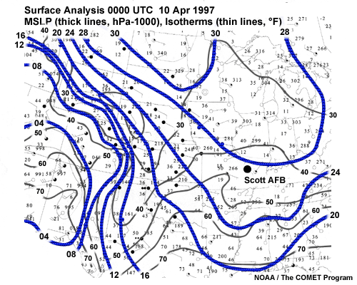
I made a quick review of my forecast.
The 0000Z surface analysis suggested that the Scott AFB region was under the influence of an anticyclone.
Scenario » Conditions Aloft
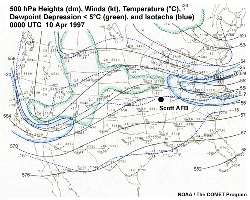
In fact, we had a sizeable ridge at 500 hPa over the region.
Scenario » 850 hPa
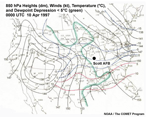
Closer inspection of the lower troposphere revealed easterly flow and dry air with wet bulb temperatures around 0°C at the surface in the rear of a retreating high, a feature that evolved into a high amplitude ridge at 850 hPa.
Scenario » Available Moisture
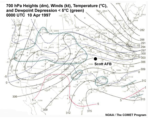
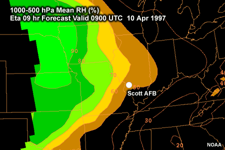
And we had a good deal of moisture upstream, a pattern reflected at 700 and 500 hPa as well.
Scenario » Lift and Moisture
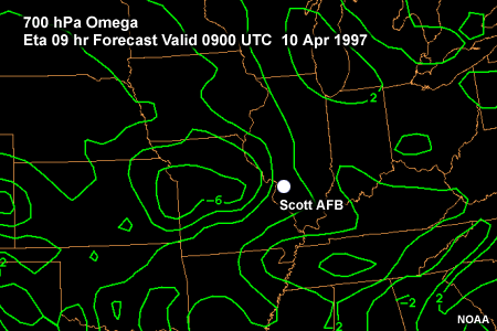
Looking at the models, the vertical motion and moisture fields revealed the likelihood of precipitation with good moisture and plenty of lift over Missouri.
Omega is the vertical velocity expressed as the rate of change of pressure with time, typically in units of microbars per second. Negative values indicate rising motions and positive values indicate sinking motions. While this can be confusing, it may help to remember that negative values are tied to falling pressure, which we typically associate with rising air.
Scenario » Frontogenesis
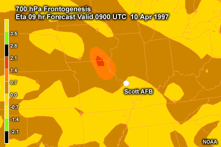
I also looked at the 700 hPa frontogenesis. I wanted to see whether we had much potential for banding. There was a region of enhanced values running northwest-to-southeast over eastern Missouri, with Scott AFB near the eastern edge. Things were looking good for some banded precip in my Area of Responsibility.
But to decide what to tell the C-5, I needed a clear distinction between a forecast of rain or snow.
Frontogenesis is a common, but very important atmospheric process. It refers to an increase in the magnitude and a change in the orientation of a thermal gradient at a level or within a layer. Frontogenesis is caused by horizontal changes in the total wind due to patterns of convergence and divergence. The increase in magnitude of the temperature gradient alters the thermal wind balance, which in turn forces a vertical-motion response in the atmosphere. Air on the warm side of the thermal gradient rises and cools, while air on the cool side sinks and warms. These motions act to weaken the thermal gradient and restore the thermal wind balance. Vertical motions forced by frontogenesis can result in a distinct band of heavy precipitation within surrounding lighter precipitation.
Scenario » Base Soundings
I pulled up the model soundings for the Base and followed their progress from initialization at 0000Z through the current time and out to 1800Z. When I looped the soundings, they looked like an inverted zipper. The temperature and dewpoint traces closed in on the wet bulb trace from aloft and moved downward toward the surface. More importantly, the wet bulb temperature throughout that layer was close to 0°C. Near the end of the loop, the near-surface layer was cooling from a few degrees above freezing down to the 0°C isotherm.
Scenario » Decision Time
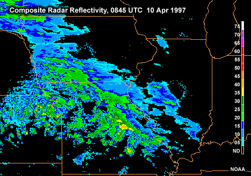
The time was 0935Z, and the flight was due in 30 minutes. The 0900Z obs from Scott showed visibility of 7 miles with a broken ceiling of 10,000 feet. I took one more look at the St. Louis radar, then I picked up the phone to call the duty officer.
What do you think?
Would conditions remain above minimums for another half hour?
Or
should Master Sergeant Slade revise his forecast and redirect the C-5?
Introduction
At the end of this section you should be able to do the following things:
- Recall the operational definition of a precipitation band
- Describe the relationship between instantaneous and accumulated bands of precipitation
- Recall the basic requirements for precipitation and the role of atmospheric stability
Introduction » Discussion
Introduction » Discussion » Mesoscale Precipitation Bands
Mesoscale precipitation bands present a significant challenge to modern operational weather forecasters. Basic meteorological training gives only brief exposure to this problem, and NWP models have difficulties generating accurate forecasts of narrow precipitation bands. This module will explore the synoptic environments and mesoscale processes that lead to banded precipitation.
Introduction » Discussion » What Is a Precipitation Band?
The term "precipitation band" has been defined as either an instantaneous feature on a radar image or as an elongated region of accumulated precipitation. Novak and his colleagues (2002) defined a single precipitation band to be at least 250 km in length and no more than 100 km in width. Their definition relies on thresholds for radar reflectivity maintained over a minimum time period.
We will tend toward the instantaneous feature definition in this discussion. In either case, significant precipitation bands of either type in the midlatitudes typically occur in conjunction with an extratropical cyclone. In particular, the frontal zones of extratropical cyclones are often closely associated with many precipitation bands. Therefore, it is necessary to briefly review cyclone structures, especially as they relate to the generation and maintenance of precipitation bands.
Introduction » Discussion » Accumulated Precipitation

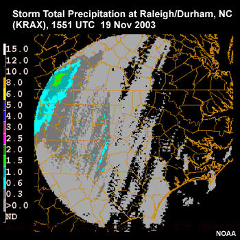
These dimensions can also apply to the accumulated, storm-total precipitation generated by a single storm. For example, this plot shows a band of snow that fell across southern Missouri and Illinois on 13-14 March 1999. However, such elongated regions of accumulated precipitation do not always result from an organized mesoscale precipitation band.
Introduction » Discussion » Instantaneous vs. Accumulated Precipitation
In a similar fashion, it is important to realize that instantaneous precipitation bands may or may not result in a banded accumulation of precipitation. The pattern of accumulated precipitation depends on the motion of the instantaneous band relative to its orientation. This radar loop shows a squall line moving perpendicular to its length. Note that as the squall line sweeps from west to east, individual cells move north-northeast, as determined by the wind-shear vector.
To learn more about squall lines and their motion, see the module Severe Convection II: Mesoscale Convective Systems (www.meted.ucar.edu/mesoprim/severe2).
The passage of the squall line resulted in a broad band of accumulated precipitation, as shown in this plot of storm-total precipitation.
Conversely, when an instantaneous band moves parallel to its length, narrow bands of accumulated precipitation may result.
The passage of single cells of intense precipitation may also result in narrow bands of accumulated precipitation. The north-northeast bands within the storm-total precipitation plot reflect the passage of individual cells within the squall line.
To learn more about squall lines and their motion, see the module Severe Convection II: Mesoscale Convective Systems (www.meted.ucar.edu/mesoprim/severe2).
Introduction » Discussion » Precipitation Basics
Before we delve into precipitation banding, lets revisit briefly those components necessary for rain or snow formation, chiefly moistureand lift. While these two ingredients are sufficient to generate rain or snow, instability must also be present if the precipitation is to be convective.
Introduction » Discussion » Moisture
When forecasting precipitation, it is best to begin with an assessment of the moisture available in the atmosphere. The atmosphere may well be rising, but in the absence of moisture for cloud development, all you will have is dry ascent, such as a thermal.
This plot comes from the scenario that started the module. It shows mean relative humidity in the 1000-500 hPa layer. Note the values exceeding 90% across eastern Nebraska and western Iowa. Considerable moisture is assumed to be present when the relative humidity exceeds 80% at a given level. Nucleation begins in the atmosphere at around this value.
Introduction » Discussion » Lift
With adequate moisture, we need rising motion to generate clouds and precipitation. After all, the atmosphere may be saturated, but in the absence of ascent, all you may have is a cloud or fog.
We can look at the output from an NWP model and assess the vertical motion fields to find ascent and descent. For example, this plot shows vertical velocity, expressed as Omega, at 700 hPa for the scenario case that started this module. Negative values indicate upward motion. Notice the region of ascending flow across central Missouri.
Once we have defined regions of sufficient moisture and lift, we may look more closely at these areas in order to assess the likelihood of mesoscale banding. Precipitation banding results from mechanisms that organize either the lift or the moisture into narrow regions.
Omega is the vertical velocity expressed as the rate of change of pressure with time, typically in units of microbars per second. Negative values indicate rising motions and positive values indicate sinking motions. While this can be confusing, it may help to remember that negative values are tied to falling pressure values as altitude increases.
Introduction » Discussion » Precipitation in Cyclones
Models of midlatitude cyclones provide a good place to start a discussion of banded precipitation. The Norwegian Cyclone Model, for example, exhibits a fairly broad precipitation area associated with the leading warm front and a narrower mesoscale precipitation band associated with the trailing cold front. Obviously, processes at work in cyclones lead to banded precipitation. It follows that being familiar with the Norwegian model of frontal and precipitation structures will help us understand the generation and organization of mesoscale precipitation systems.
Introduction » Discussion » Banded Precipitation and Convection
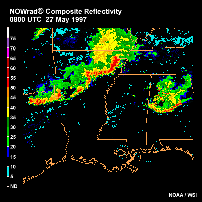
A relationship often exists between banded precipitation and convection in both the warm and cold seasons. For example, this radar plot shows bow echoes within a longer squall line that occurred over Arkansas. However, we will not address Mesoscale Convective Systems here as they receive extensive treatment in the Mesoscale Primer module Severe Convection II: Mesoscale Convective Systems.
For an extensive treatment of warm season linear convection, see the Mesoscale Primer module Severe Convection II: Mesoscale Convective Systems (www.meted.ucar.edu/mesoprim/severe2).
Introduction » Questions
Introduction » Questions » Question
Question 1
Which of the following factors are required for precipitation to occur? (Choose all that apply.)
The correct answers are a) and b).
Generally, a high relative humidity is sufficient for condensation to occur, but only a cloud will form unless there is ascent and cooling. Instability can lead to showery precipitation and frontogenensis may provide lift, but neither are required for precipitation to occur.
Introduction » Questions » Question
Question 2
A band of precipitation in a radar scan will always result in a banded accumulation of precipitation over several hours. (Choose the best answer.)
The correct answer is False.
If an instantaneous band of precipitation, detected by radar, moves in a direction perpendicular to its length, the resulting accumulation could be quite wide. This is akin to the sweeping motion of a windshield wiper.
Introduction » Questions » Question
Question 3
A banded accumulation of precipitation always results from an instantaneous band of precipitation. (Choose the best answer.)
The correct answer is False.
A banded accumulation of precipitation may also result from the passage of a convective cell, or a series of convective cells that follow the same path.
Synoptic Environments Favoring Banded Precipitation
At the end of this section you should be able to do the following things:
With regard to the Norwegian Cyclone Model:
- Recall and describe the different types of fronts in the Norwegian cyclone model
- Describe the typical precipitation field associated with each kind of front
- Distinguish an anafront from a katafront in forecast products
- Distinguish a cold occluded front from a warm occluded front in forecast products
With regard to the conveyor belt model of cyclones:
- Recall and describe the types of air streams in the conveyor belt model of midlatitude cyclones
- Describe the relationship between air streams and fronts
- Describe the relationship between air streams and mesoscale banded precipitation
- Recognize different air streams in satellite images and forecast products
- Recall what a trowal is and where it occurs
- Describe the relationship between the trowal and banded precipitation
- Describe the trowal signature in forecast products
- Locate a trowal on satellite images and forecast products
Synoptic Environments Favoring Banded Precipitation » Introduction
Synoptic Environments Favoring Banded Precipitation » Introduction » Introduction
This section briefly reviews mesoscale precipitation bands in the context of the larger synoptic-scale cyclones in which they are found. We will not attempt an exhaustive treatment of cyclone structures, as you are likely already aware of those topics. Instead, we will focus on how mesoscale bands form within various cyclones.
Synoptic Environments Favoring Banded Precipitation » Introduction » Models of Cyclone Structure
In the early 1900s, a group of Norwegian meteorologists proposed a model of cyclone morphology and evolution that persists to this day. Although highly descriptive and limited by geography and available data, the Norwegian Cyclone Model has provided a valid framework around which synoptic meteorology has grown up and matured in the intervening decades.
As you view the different aspects of cyclone models, keep in mind that although each of the conceptual models is useful in its own way, none of them has a lock on describing all of the forms that an individual cyclone and its associated precipitation structures may take. So don't place too much stock in any single cyclone model to describe precipitation structures. Instead, look for those dynamic mechanisms that generate and organize banded precipitation.
Synoptic Environments Favoring Banded Precipitation » Norwegian Cyclone Model
Synoptic Environments Favoring Banded Precipitation » Norwegian Cyclone Model » Introduction
The Norwegian Cyclone Model presents the atmosphere as a juxtaposition of air masses, separated by boundaries where the temperature changes greatly over a short horizontal distance. These boundaries are called fronts. A leading warm front is followed by a faster cold front. As the cold front outpaces the forward motion of the warm front, they collide and form an occluded front.
In the Norwegian model, each front is viewed as a sloping material surface, a hard boundary like an enormous sheet of glass that separates a warmer air mass from a colder one. In this model, motions near fronts are forced upward or downward along the sloping frontal surfaces. In modern views of fronts, surfaces of potential temperature or moist potential temperature act much like the material surfaces that the Norwegians envisioned.
As you know, fronts can generally be classified as cold fronts, warm fronts, occluded fronts, or stationary fronts. Precipitation in cyclones is strongly organized by these frontal structures. Hence, consideration of the structure and processes associated with fronts will help identify where and how banded precipitation occurs in cyclones.
Synoptic Environments Favoring Banded Precipitation » Norwegian Cyclone Model » Warm Fronts
In the case of the warm front, moist warm-sector air flows along and up the broad extent of the warm frontal slope. The slope of the warm frontal zone is relatively gentle, much less steep than that of a cold front. As a result, precipitation is often continuous in character and tends to fall in a wide band north of the surface warm front location.
Synoptic Environments Favoring Banded Precipitation » Norwegian Cyclone Model » Example
We know now that mesoscale bands may form within the broad region of precipitation associated with a warm front.
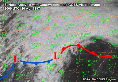
In this example from our scenario case, satellite imagery shows a broad band of clouds and precipitation north of the warm front. The warm front, associated with a surface cyclone over the southern Rockies, extends from southeastern Kansas across southern Missouri at 2000 UTC on 10 April 1997.
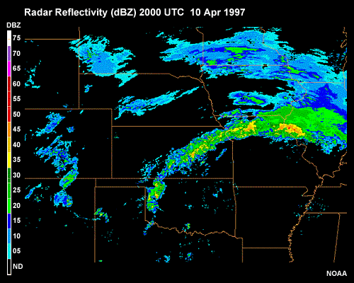
At this time, a band of moderate-to-heavy precipitation is located north of the warm front from east-central Kansas across northern Missouri and into central Illinois.
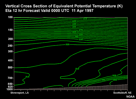
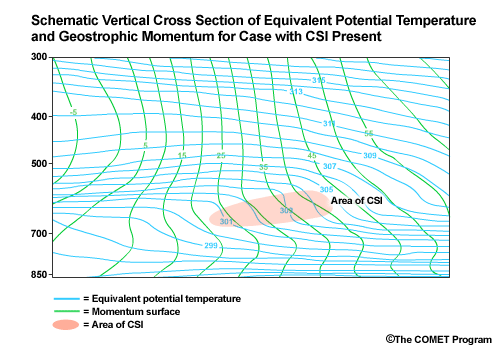
The mesoscale band in this case resulted from the instability in the air mass flowing up and over the warm front. We can see the weak stability shown by the near-vertical contours of equivalent potential temperature in this vertical cross section of the warm front. The result was elevated convection above the warm front, leading to a relatively narrow band of precipitation.
Synoptic Environments Favoring Banded Precipitation » Norwegian Cyclone Model » Question
Question 4
Precipitation associated with passage of a warm front tends to fall on the _____ side of the surface front. (Choose the best answer.)
The correct answer is a) cold.
Precipitation occurs when warm moist air ascends a shallow slope over cooler, denser air. Thus, precipitation falls on the cool side of the surface warm front.
Synoptic Environments Favoring Banded Precipitation » Norwegian Cyclone Model » Question
Question 5
Mesoscale banded precipitation _____ occurs in conjunction with a warm front. Choose the best answer.
The correct answer is a) sometimes.
Precipitation associated with a warm front typically forms a broad shield, though in some cases elevated convection may lead to banded precipitation.
Synoptic Environments Favoring Banded Precipitation » Norwegian Cyclone Model » Cold Fronts
Cold fronts typically have a steeper slope than warm fronts. Consequently, motions along such a frontal zone are often much stronger, both upward and downward. The outcome is a narrow band of convective precipitation that is showery in character. All things being equal, this is where we would usually think to look first for thunderstorm development within an extratropical cyclone.
Synoptic Environments Favoring Banded Precipitation » Norwegian Cyclone Model » Cold Katafronts
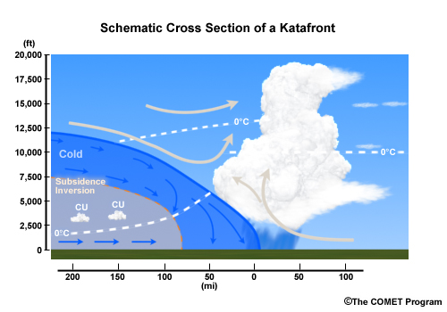
Following the introduction of the Norwegian model, observational studies of cyclones and frontal zones determined that there were two primary types of cold frontal zones: the anafront and katafront. The katafront is one where the component of flow perpendicular to the frontal zone is faster than the frontal speed and is downward toward the surface of the earth. Remember that the flow in the frontal zone is largely parallel to the front, with only a small perpendicular component.
The downward flow leads to compression and warming and subsequent evaporation of any moisture or cloud droplets. Upward motion will be forced largely by boundary layer convergence near the surface front. This results in a long, narrow band of precipitation oriented along and parallel to the surface front. The mesoscale precipitation band in the original Norwegian Cyclone Model results from a katafront.
Synoptic Environments Favoring Banded Precipitation » Norwegian Cyclone Model » Cold Anafronts
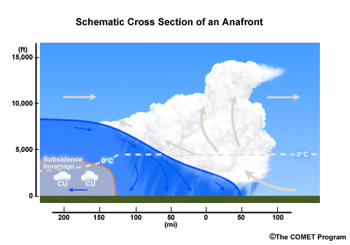
Anafront structure occurs when a front advances faster than the flow in which it is embedded. How does that happen? In the case of the anafront, the concept of the material surface no longer applies. The front advances due to wave propagation, and the flow responds accordingly. Warm air flows up the face of the frontal surface, which is typically not as steep as in a katafront. This upward motion is not as vigorous and occurs over a broader area, generating an expanded precipitation shield. A cold anafront is akin to a warm front in reverse.
Synoptic Environments Favoring Banded Precipitation » Norwegian Cyclone Model » Anafront Versus Katafront
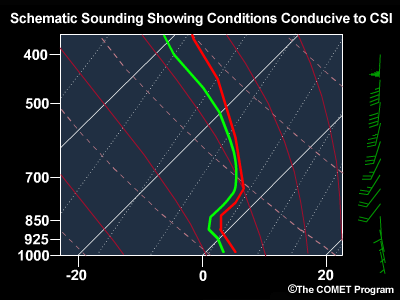
From an operational perspective, the sensible weather associated with an anafront differs markedly from that associated with a katafront. An anafront generally produces heavier rainfall, but convection ahead of a katafront may produce heavy banded precipitation. Typically, passage of an anafront is marked by a sharp drop in temperature at the surface, but not humidity, while passage of a katafront is marked by a sharp drop in humidity, but not temperature. Examining a sounding taken through the front is one way of distinguishing an anafront from a katafront.
Question 6
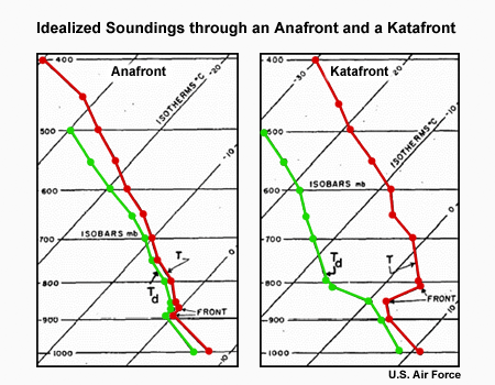
This plot shows two idealized soundings, one is for an anafront and the other for a katafront. Which is which? (Choose the best answer.)
The correct answer is a).
The anafront sounding, on the left, shows a weak frontal inversion and a small dewpoint depression, indicating a deep layer of high relative humidity. The katafront sounding, on the right, shows a rather strong inversion aloft, which has been enhanced by subsidence along the frontal zone. This subsidence also creates a substantial layer of dry air, shown by the large dewpoint depression above the inversion.
Please continue watchiong the video above.
Bear in mind that the characteristics of a cold front can change over its lifetime. In the early stages of cyclogenesis, a cold front is an anafront over most of its length. The katafront forms later as the system starts to occlude, spreading outward from the low with time. Finally, as the cyclone fully occludes, the cold front tends to become a weak anafront.
Synoptic Environments Favoring Banded Precipitation » Norwegian Cyclone Model » Question
Question 7
Banded precipitation is more likely to occur ahead of the surface cold front in the case of a(n) _____. (Choose the best answer.)
The correct answer is b) katafront.
Flow down the frontal surface in the case of the katafront will keep the precipitation near and ahead of the surface front.
Synoptic Environments Favoring Banded Precipitation » Norwegian Cyclone Model » Occluded Fronts
In the Norwegian model, occluded fronts represent the collision of a cold front with a warm front. This collision occurs because warm fronts often move more slowly than the cold frontal zones that follow them. The cold front then catches up to the warm front ahead, and the occluded front is formed. This process lifts air in the warm sector away from the surface and forces the warm, moist air aloft. The outcome is often cloudiness, low visibilities, and precipitation that may range from drizzle to a thunderstorm.
It would seem clear that occluded fronts are often the focus of inclement weather, yet that is not always the case. Sometimes the passage of the surface occluded front signals the onset of precipitation and low visibilities, but other times occluded frontal passage coincides with the end of poor conditions. These differences depend largely upon whether you're dealing with a warm or cold occluded front. Although there was no real distinction between warm or cold occluded frontal types in the original Norwegian Cyclone Model, the theory left the door open to such modification, and we examine those differences here.
Synoptic Environments Favoring Banded Precipitation » Norwegian Cyclone Model » Warm Occluded Fronts
Warm occluded fronts occur when the air mass behind the trailing cold front is warmer than the air mass ahead of the leading warm front. Warm sector air is still occluded upward, but the three-dimensional structure of the warm occlusion creates a cold front aloft and ahead of the surface occluded front. Given this structure, the occluded front at the surface tends to lie behind the thickness ridge on a sea level pressure and 1000-500 hPa thickness chart. The cloudiness and precipitation that occur will typically do so ahead of the surface occluded front so that improving weather occurs after the surface occluded front passes by.
Synoptic Environments Favoring Banded Precipitation » Norwegian Cyclone Model » Cold Occluded Fronts
Cold occluded fronts occur when the air mass behind the trailing cold front is colder than the air mass ahead of the leading warm front. Warm sector air is again occluded upward, but the three-dimensional structure of the cold occlusion creates a warm front aloft (what had been the surface warm front) and behind the surface occluded front. In this situation, the occluded front tends to lie near or to the warm side of the thickness ridge on surface and 1000-500 hPa thickness charts. The cloudiness and precipitation that occur will typically do so behind the surface occluded front so that deteriorating weather occurs after the surface occluded front passes by.
Synoptic Environments Favoring Banded Precipitation » Norwegian Cyclone Model » Question
Question 8
The 1000-500 hPa thickness will be greater _____ a cold occluded front. (Choose the best answer.)
The correct answer is a) ahead of.
Because the 1000-500 hPa thickness is proportional to the mean temperature, and the coldest air lies behind the cold occluded front, the 1000-500 thickness will be greater ahead of the surface occluded front.
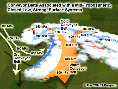
Synoptic Environments Favoring Banded Precipitation » Conveyor Belt Model
Synoptic Environments Favoring Banded Precipitation » Conveyor Belt Model » Overview

An airstream or conveyor belt model of cyclone structure and evolution has emerged in the last few decades. Unlike the earlier air mass approach of the Norwegian Cyclone Model, the conveyor belt view provides for relatively narrow ribbons of air flowing along sloping isentropic surfaces. These airstreams are defined in a system-relative-flow sense and thus represent air trajectories through the moving and evolving cyclone. Consequently, the airstreams, as they are lifted along isentropic surfaces, produce clouds and precipitation structures during various stages of midlatitude cyclone evolution. As with the Norwegian model, these airstreams also focus precipitation, but usually on the larger meso-alpha scale.
The model consists of a warm conveyor belt, a cold conveyor belt, and a dry, descending airstream. The warm conveyor belt usually transports warm air poleward and is the warm, moist air mass that is lifted over the warm front. The cold conveyor runs parallel to the warm front on its cold side. The dry airstream supplies drier, descending air behind the surface cold front, which may then ascend around the cyclone center. Although the warm conveyor belt is perhaps the most useful for describing and diagnosing where precipitation will form, the cold and dry airstreams do play a role in the organization of precipitation.
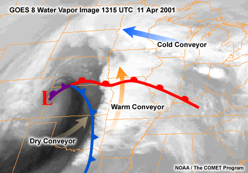
Question 9
This satellite image shows water vapor for a mature cyclone over the Midwest on 11 April 2001 along with analyzed fronts. The warm, cold, and dry airstreams are all easily distinguished.
On the image below:
- Use the blue pen to show the cold conveyor.
- Use the red pen to show the warm conveyor.
- Use the yellow pen to show the dry conveyor.
When you have finished, select Done.
Compare your answer to the answer below.
Question 10
This plot shows a model-analyzed, south-to-north vertical cross section along the warm conveyor belt from Little Rock, Arkansas to Des Moines, Iowa.
On the image below:
- Use the pen to mark location of the warm conveyor belt.
When you have finished, select Done.
Compare your answer to the answer below.
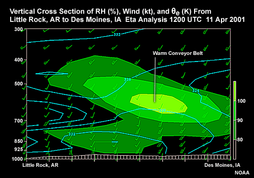
The center of the warm conveyor belt is located between approximately 800 and 500 hPa. It is marked by strong south-southwesterly flow in this layer.
Question 11
This plot shows a WSW-ENE vertical cross section along the cold conveyor belt.
On the image below:
- Use the pen to mark location of the cold conveyor belt.
When you have finished, select Done.
Compare your answer to the answer below.
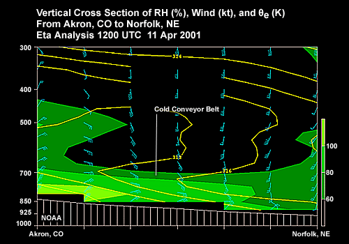
The cold conveyor belt is located between approximately 800 and 600 hPa and begins where the layer of low-level easterly flow becomes sufficiently deep.
Synoptic Environments Favoring Banded Precipitation » Conveyor Belt Model » Warm Conveyor Belt
As its name implies, the warm conveyor belt is a warm airstream, often flowing poleward along most of its length. Originating in the warm sector of midlatitude cyclones, the warm conveyor belt slopes upward as it flows poleward, along and ahead of the cyclones cold front. It is then lifted as it flows up and over the warm front.
Synoptic Environments Favoring Banded Precipitation » Conveyor Belt Model » Forward-Sloping Warm Conveyor Belt
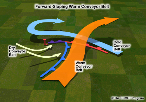
The forward-sloping warm conveyor belt is similar in many ways to a cold katafront, where the flow perpendicular to the cold front moves forward more rapidly than the frontal zone. Note that the three-dimensional flow of the warm conveyor belt is mostly parallel to the cold front with just a slight component perpendicular to the front to yield the katafront structure.
A forward-sloping warm conveyor tends to confine clouds and precipitation along and ahead of the surface cold front. This effect may be enhanced if dry air also descends above the cold frontal surface and overruns the underlying warm conveyor belt. The resulting instability leads to precipitation, possibly banded, in the warm sector.
This type of system commonly occurs downstream of a diffluent trough axis in the flow aloft.
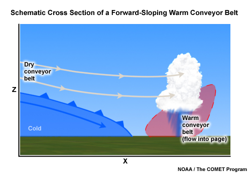
A pronounced case of the forward-sloping warm conveyor belt results in the split-front structure. Strong advection of low-humidity air down the katafront surface leads to generation of potential instability. Consequently, a shelf of cloudiness forms along and ahead of the surface cold front. Heavy convective rain may fall from this deeper shelf of cloudiness. Subsequent passage of the surface front may be associated with a dry cold frontal passage or just a narrow line of precipitation near the front.
Synoptic Environments Favoring Banded Precipitation » Conveyor Belt Model » Rearward-Sloping Warm Conveyor Belt
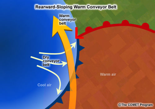
The rearward-sloping warm conveyor belt is similar to a cold anafront. Most of the warm conveyor flow is parallel to the front with a slight component up and over the advancing cold air. Thus, flow ascends the isentropic surfaces of the frontal zone. The rearward-sloping conveyor structure leads to heavy convective precipitation at the time of frontal passage, followed by lighter, more stratiform precipitation behind the surface front.
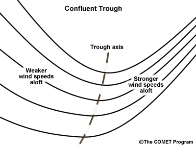
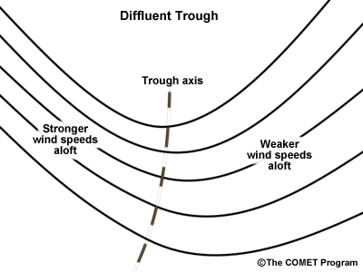
This type of system commonly occurs downstream of a confluent trough axis in the flow aloft.
Synoptic Environments Favoring Banded Precipitation » Conveyor Belt Model » Trowal (Warm Conveyor Belt)
In well-developed mature cyclones, a portion of the warm conveyor belt will turn cyclonically and be pulled into the circulation. This creates a trough of warm air aloft (a trowal) that is often relatively narrow and focused.
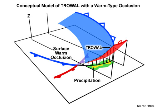
The trowal is a sloping canyon formed by ascending warm air with relatively cooler air in place on both sides. The trowal originates at the apex of the warm sector in the pre-occlusion phase of a cyclone. It gradually rises above the surface occluded front. Often, the outcome is a region of precipitation well separated from the warm sector in the wrap-around portion of a cyclone. When the trowal is present in a cyclone, it contributes to the cloudiness and enhances the precipitation associated with the comma-head signature of a cyclone.
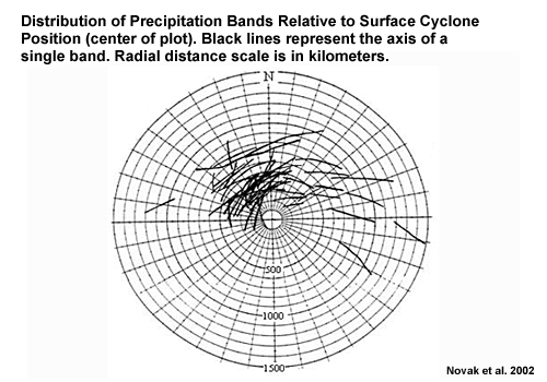
This plot shows the results of a 5-year cold-season climatology in the northeast U.S. The lines in the plot show the axes of snowbands relative to the center of their respective cyclones. We can see that the majority of the bands fall in the northwest quadrant of the plot, 300-500 kilometers from the cyclone center, and are oriented roughly northeast-southwest. This plot confirms that heavy precipitation bands frequently form in the occluded, wrap-around portion of a cyclone, far from the warm and cold fronts of the Norwegian Cyclone Model.
Synoptic Environments Favoring Banded Precipitation » Conveyor Belt Model » Example
Question 12
So what does a trowal look like? We will look at an example that was studied by Graves and his colleagues. This particular trowal developed in conjunction with strong cyclogenesis on 10 November 1998 in the upper Midwest.
On the image below:
- Use the pen to mark the location of where you would expect to find a trowal.
When you have finished, select Done.
Compare your answer to the answer below.
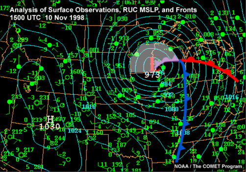
The trowal would be expected to form in the occluded portion of the cyclone, over Wisconsin and Minnesota.
In this case, the trowal structure resulted in heavy banded snowfall along the South Dakota/Minnesota border. Note that the band of precipitation stays anchored over Sioux Falls throughout the loop. The precipitation bands are located to the northwest of the surface low and on the west side of the dry airstream, which is typical of many trowal events.
Question 13
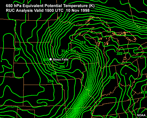
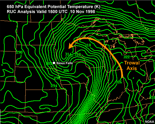
A trowal can usually be detected by looking at a midlevel (700-600 hPa) θeanalysis. This plot shows the 650 hPa θe.
On the image below:
- Use the pen, draw a line down the center of the trowal
When you have finished, select Done.
Compare your answer to the answer below.
Please continue wachting the video above.
Note the cyclonically turning tongue of warmer temperatures curving from Michigan to Minnesota. This results in a characteristic S-shape for the moist isentropes at midlevels. These warm temperatures also correspond to the cyclonically turning portion of the warm conveyor belt. The contours indicate that the trowal ascends sharply near the southwest corner of Minnesota where it reaches the end of a box-canyon created by three-dimensional airstreams.
Question 14
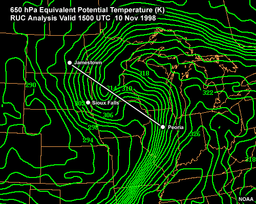
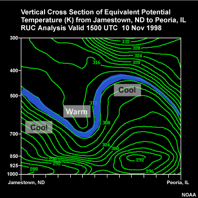
Now let's look at a cross section from Jamestown, North Dakota to Peoria, Illinois.
On the image below:
- Use the pen to locate the trowal in this cross section of equivalent potential temperature.
When you have finished, select Done.
Compare your answer to the answer below.
Please continue wachting the video above.
This cross section shows a canyon of warmer air walled in by cooler air. That is the trowal.
In this IR satellite loop, have a look at eastern South Dakota. Note the enhancement and persistence of deep cloudiness just north of the cyclone comma head as the entire system evolves and moves northeastward. This is the western end of the trowal and an area of significant and persistent ascent during this time period.
Synoptic Environments Favoring Banded Precipitation » Questions
Synoptic Environments Favoring Banded Precipitation » Questions » Question
Question 15
Select the correct words to complete the sentence.
The correct answer shown above.
With a warm occluded front, the coldest air mass lies ahead of the warm front. Therefore, when the fronts occlude, the cold front rides up and over the warm front. This places the precipitation field ahead of the surface occluded front.
Synoptic Environments Favoring Banded Precipitation » Questions » Question
Question 16
Select the correct words to complete the sentence.
The correct answer shown above.
With an anafront, warm sector air flows up over the cold front. The precipitation field is characterized by line convection along the surface front and stratiform precipitation behind the surface front.
Synoptic Environments Favoring Banded Precipitation » Questions » Question
Question 17
Select the correct words to complete the sentence.
The correct answer shown above.
A dry conveyor belt flows down the frontal zone and downward out ahead of the cold front. The air dries as it descends. This flow creates instability in the warm sector along and ahead of the cold front as cool, dry air flows over warm, moist air. Passage of the surface cold front results in improving Weather.
Synoptic Environments Favoring Banded Precipitation » Questions » Question
Question 18
Select the correct words to complete the sentence.
The correct answer shown above.
Synoptic Environments Favoring Banded Precipitation » Questions » Question
Question 19
Precipitation bands associated with a trowal typically form in which quadrant, with respect to the center of the surface cyclone? (Choose the best answer.)
The correct answer is d) Northwest.
A climatology of heavy banded snowfall in the northeast U.S. showed that most bands occurred 300-500 km from the surface low in the northwestern quadrant.
Dominant Mesoscale Banding Processes
At the end of this section you should be able to do the following things:
With regard to deformation and frontogenesis:
- Define the terms: deformation, frontogenesis, frontolysis
- Describe how deformation leads to frontogenesis
- Describe the vertical motions associated with frontogenesis
- Describe how frontogenesis leads banded precipitation
- Recognize and diagnose deformation and frontogenesis in forecast products
With regard to melting and evaporation-induced effects:
- Describe circulations induced by melting and evaporation in the lower troposphere
- Describe the relationship between melt/evaporation-induced circulations, frontogenesis, and banded precip
- Recognize and diagnose banded precipitation forced by melt/evaporation-induced circulations in forecast products
With regard to frontal merger:
- Define frontal merger
- Describe the difference between frontal merger and frontal occlusion
- Describe a typical synoptic setting for frontal merger and its relationship with midlatitude cyclones
- Describe the relationship between frontal merger and banded precipitation
- Recognize and diagnose frontal merger in forecast products
With regard to CSI and slantwise convection:
- Describe the relationship between CSI and slantwise convection
- Describe the atmospheric conditions conducive to CSI
- Describe what atmospheric conditions lead to low inertial stability
- Recognize and diagnose CSI and slantwise convection with cross sectional analyses.
Dominant Mesoscale Banding Processes » Introduction
Not all banded precipitation occurs within a midlatitude cyclone. For example, in the warm season over the central U.S., lines of thunderstorms may form in the absence of an organized cyclonic circulation. Likewise, bands of convective snowfall may occur downstream of the Great Lakes even though the responsible cold northerlies are due to a surface low hundreds of kilometers away. Sea-breeze and land-breeze circulations near the coast are two more examples of mesoscale banded precipitation that do not require a cyclone. Non-cyclogenic processes are dealt with in other modules.
In this module, we focus on those processes responsible for banding within extratropical cyclones. The previous section addressed banded precipitation associated with isentropic ascent up frontal surfaces. However, banded precipitation also occurs due to other processes at work in extratropical cyclones. This section explores some of those processes.
Please see the References section for an annotated list of related COMET modules.
Dominant Mesoscale Banding Processes » Deformation and Frontogenesis
Dominant Mesoscale Banding Processes » Deformation and Frontogenesis » What is Deformation?
Regions of deformation should be monitored for banded precipitation. Deformation is the process by which an airstream tends to stretch or alter the distribution of a tracer embedded in the flow, such as moisture. Under certain circumstances, deformation leads to frontogenesis, which can focus precipitation into a narrow band.
Deformation can arise in various ways. This figure illustrates one way, whereby two conflicting airstreams are directed toward one another in the middle or upper levels of the atmosphere. At a great distance, neither flow is disturbed, but as each flow approaches the other, they split and fan out in a diffluent pattern. A col point is generated in the center of the deformation field, at the intersection of the axis of contraction with the axis of dilatation.
Consider how the clouds are spread out along the axis of dilatation if the southeasterly flow is moist and the northwesterly flow is dry, as shown here. Over time, the moisture gradient increases along the axis of contraction and spreads along the axis of dilatation. Deformation can and does occur in the conveyor belts discussed previously.
For example, the splitting warm conveyor belt in a trowal leads to deformation along an axis perpendicular to the trowal, as shown in this figure. Another deformation zone occurs with confluence between the dry and warm conveyor belts along the back edge of the cold frontal clouds, leading to contraction of the moisture gradient.
Dominant Mesoscale Banding Processes » Deformation and Frontogenesis » Frontogenesis and Frontolysis
Deformation can also affect temperature fields, leading to frontogenesis. Frontogenesis is a measure of the change with time in the magnitude of a temperature gradient. When a temperature gradient strengthens with time, frontogenesis values are positive, and we say that frontogenesis is occurring. This plot shows a case where deformation leads to frontogenesis. Note that the isotherms are oriented perpendicular to the axis of contraction.
When a temperature gradient weakens with time, frontogenesis values are negative, and we say that frontolysis is occurring. Frontolysis may occur when isotherms are oriented perpendicular to the axis of dilatation.
Dominant Mesoscale Banding Processes » Deformation and Frontogenesis » Vertical Motions Induced by Frontogenesis
When frontogenesis or frontolysis alters the thermal gradient, there is a direct impact on the pressure or height distribution in the region of frontogenesis. This can be seen in the change in thicknesses across the region of frontogenesis. Because of the atmosphere's strong tendency to maintain geostrophic balance, this change in the thermal structure forces ascent and descent to occur in regions of frontogenesis. Ascent occurs on the warm side, which adiabatically cools the rising flow. Simultaneously, descent on the cool side adiabatically warms the flow there. If the air is moist, these induced vertical motions support cloud formation and precipitation along the axis of dilatation. Consequently, deformation and frontogenesis are very important in organizing precipitation into mesoscale bands.
Dominant Mesoscale Banding Processes » Case Example
Question 20
This plot shows streamlines, relative humidity, and pressure on a 298-kelvin isentropic surface.
On the image below:
- Use the pen to mark where you expect to find deformation.
When you have finished, select Done.
Compare your answer to the answer below.
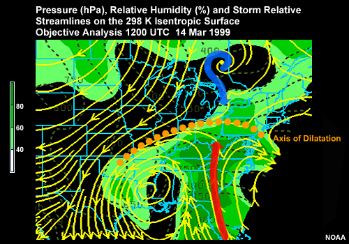
In this instance, deformation will occur where the warm, moist airstream coming up from the south encounters the cool dry air coming out of the north. The axis of dilatation runs from Oklahoma through the upper Midwest and east through Pennsylvania. This area is roughly delineated by the northern edge of higher relative humidities.
Question 21
On the image below:
- Use the pen to mark where would you expect to find significant frontogenesis.
When you have finished, select Done.
Compare your answer to the answer below.

As we expect, positive values of frontogenesis are concentrated right along the axis of dilatation. However, frontogenesis does not signal the location of strongest vertical motion.
Question 22
On the image below:
- Use the pen to mark the region where you expect to find the strongest ascent.
When you have finished, select Done.
Compare your answer to the answer below.
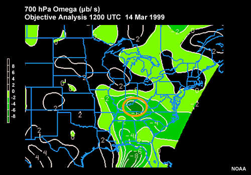
While positive frontogenesis values are associated with rising motion, the maximum ascent is usually found adjacent to the frontogenesis maximum and on its warm side. In this case, the maximum rates of vertical motion occurred to the south, in southern Illinois and Indiana.
Question 23
On the image below:
- Given the relative humidity and the ascent, use the pen to mark the map where you would expect to find a band of precipitation.
When you have finished, select Done.
Compare your answer to the information below.
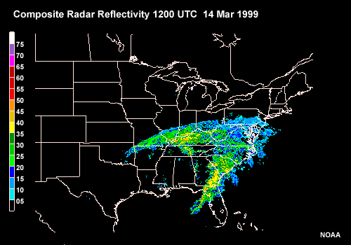
In the Northern Hemisphere, the western portion of the axis of dilatation is a place to watch carefully for the creation of narrow bands of rain and snowfall. In this case, note the precipitation that occurs in conjunction with deformation in southern Illinois and Indiana.
Frontogenesis may also play a prominent role in the development and evolution of warm and cold fronts in cyclones. While a complete treatment is beyond the scope of this module, it is important to recognize that the thermal gradients within the warm and cold frontal zones are important places for frontogenesis to force vertical motion and organize precipitation.
Dominant Mesoscale Banding Processes » Evaporation and Melting-Induced Effects
Dominant Mesoscale Banding Processes » Evaporation and Melting-Induced Effects » Cooling-Induced Downdrafts
Evaporation and melting-induced circulations can act to focus precipitation into mesoscale bands. When a dry layer exists near the surface, frozen precipitation, especially snow, falling into it will melt and/or evaporate. This process has several effects on the dry near-surface atmosphere:
- It cools down to near or below freezing
- It moistens, allowing later snowflakes to fall farther before evaporation
- It becomes dominated by a mesoscale downdraft, induced by evaporative cooling aloft
A thermodynamic diagram, such as a Stuve or skew-T chart, is ideal to illustrate these changes. The sort of sounding evolution depicted here is the kind that forecasters should look for in real-time balloon flights as well as model output.
Notice the progression in this animation. As snow starts to fall, it first melts, then evaporates before reaching the surface. As a result, the atmosphere cools and moistens from the top downward. Once the atmosphere is completely saturated, no further cooling can occur by evaporation. However, this does not rule out cooling through melting. Even after the atmosphere becomes saturated, additional cooling can still occur while the temperature is still above freezing. Like evaporating raindrops or sublimating snowflakes, melting can rob the air of heat energy. In order to melt ice, more heat must be taken from the surrounding air. Notice in the animation that melting-induced cooling continues after saturation is achieved so that by the end of the animation the temperature profile is nearly isothermal at 0°C.
When these processes occur in a synoptic environment with continuous precipitation, the result is a continuous downdraft.
Dominant Mesoscale Banding Processes » Evaporation and Melting-Induced Effects » Cooling-Induced Frontogenesis
In addition to generating a downdraft, cooling the air on the cold side of a front increases the temperature gradient. The resulting frontogenesis strengthens vertical motions along the front. Thus melting and evaporation lead to a mesoscale convergence zone at the surface. Consequently, warm air is forced up and over the cold air, creating a mesoscale version of the synoptic cold front, which results in banded precipitation.
Banded precipitation of this type often occurs when low-level temperatures are close to freezing. Thus, such events frequently begin as rainfall and change over to snow. Furthermore, surface frontal zones often coincide with the spatial transition from rain to snow. When this occurs, the heaviest precipitation falls in a band oriented along and parallel to the frontal zone, in the vicinity of the 0°C surface wet bulb isotherm.
Dominant Mesoscale Banding Processes » Case Example
Dominant Mesoscale Banding Processes » Case Example » Forecast Challenge
The scenario that started this module examined a case of banded precipitation that struck Scott Air Force Base and the St. Louis region on 10 April 1997. Light precipitation was in the forecast. This is not surprising, given that model progs indicated deep moisture and weak ascent associated with an approaching trough. The challenge of the forecast was twofold: (1) to predict when the rain would change over to snow and (2) to predict if and where the precipitation would be banded. Evaporative and melt-induced cooling played a large role in that forecast challenge. The scenario focused on the changeover from rain to snow. Now let's look at the question of banding.
Dominant Mesoscale Banding Processes » Case Example » Introduction - Temperature and Precipitation
Question 24
This plot depicts a 12 hour forecast of wind, temperature, and 6 hour accumulated precipitation, valid at 1200 UTC on 10 April 1997.
On the image below:
- Use the pen to outline the region where you might expect evaporative and melt-induced circulations.
When you have finished, select Done.
Compare your answer to the answer below.
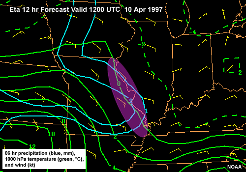
Oval in eastern MO, in the precip field, and including just west of the 0-degree isotherm
Conditions in eastern Missouri show a temperature just above freezing coinciding with light precipitation. This is the region most prone to evaporative and melting-induced cooling.
When we look at a 24 hour loop, we see rapid cooling at the surface in eastern Missouri, with temperatures near 0°C at 12 and 18 hours of simulation. Meanwhile, light precipitation amounts are forecast in this vicinity from 1200 UTC on 10 April through 0000 UTC on 11 April. This suggests that the model predicts some sort of liquid/frozen boundary in precipitation in this region.
Dominant Mesoscale Banding Processes » Case Example » Exercise - Model Soundings
This loop of soundings from St. Louis, Missouri accompanies the surface plots we just examined.
The loop of forecast soundings looks like an inverted zipper. Over time the temperature and dewpoint traces close in on the wet bulb trace from aloft, moving downward toward the surface. More importantly, the wet bulb temperature throughout that layer hovers near 0°C. Near the end of the loop, the near-surface layer cools from a few degrees above freezing down to the 0°C isotherm. In short, evaporation initially moistens and cools the near-surface layer to near freezing. Once the layer is saturated, melting-induced cooling maintains the cold temperatures at very near 0°C from about the 700 hPa level down to the surface.
Dominant Mesoscale Banding Processes » Case Example » Exercise - Radar Valiation
So what happened in this event? From 1100 UTC through 1500 UTC, the time period of significant snow in the area, a persistent band of precipitation oriented WNW-ESE extended from east-central Missouri through the southern tip of Illinois, with individual reflectivity elements moving east-southeastward along the band. From 1300 through 1430 UTC the strongest reflectivity occurred in a narrow region on the southern edge of the band, where the rain/snow boundary was likely to be located, just south of St. Louis.
Dominant Mesoscale Banding Processes » Case Example » Exercise - Surface Observations
Look at the 0400-2000 UTC loop of observations centered on the area of interest. Note that mixed precipitation begins to move into the region from the west by 0900 UTC or so, and there is evidence of mixed precipitation through 1300 UTC over central MO. Temperatures in the Scott vicinity were 3 to 5°C at 0900 UTC, but wet bulbs were below 0°C at most locations. Snow showers began in the immediate vicinity by 1000 UTC, with temperatures above freezing. By 1100 UTC the surface layer was saturated, with light snow at most locations. Light to moderate snow continued through 1500 UTC. No stations at the surface to the south reported rain during this period, but surface temperatures south of St. Louis and Scott were 1 to 2°C with high relative humidities. This suggests that there was rain in the area, but that AWOS stations did not report it. By 1700 UTC, gradual warming on the west side of St. Louis had occurred, with light rain and drizzle reported at two stations. This west-to-east trend continues through 2000 UTC, with temperatures at that point well above freezing.
To summarize, in this event model forecasts predicted a broad and light precipitation field. Instead, a narrow band of precipitation occurred over parts of Missouri and Illinois. Cooling induced by melting and evaporation apparently forced local circulations that focused the precipitation in a narrow band. This band was located along the transition from rain to snow, roughly coinciding with the southern edge of the 0°C surface wet bulb temperature.
Dominant Mesoscale Banding Processes » Frontal Merger
Dominant Mesoscale Banding Processes » Frontal Merger » Process
Frontal merger is the joining of frontal zones that are sloped in roughly the same direction. This contrasts with the development of an occluded front, which is formed by the merger of frontal zones that slope in opposite directions. This conceptual animation shows an example where an advancing warm front climbs up a stationary front. The additional lift generates a narrow band of precipitation.
Dominant Mesoscale Banding Processes » Frontal Merger » Synoptic Setting
In March of 1992 Neiman and his colleagues observed frontal merger during an extensively documented field experiment. In this case, a warm front associated with a midlatitude cyclone rode up over a stationary front. Subsequently, an arctic air mass dropped south out of Canada and bulldozed its way first under the stationary front, and then under the cyclone. As the arctic air mass advanced southward and encountered fronts, it essentially pushed under the warmer air masses. Consequently, air masses and fronts to the south decoupled from the surface and rode up over the cold dense arctic air. The additional lift produced heavy banded precipitation.
Dominant Mesoscale Banding Processes » Frontal Merger » Diagnosis
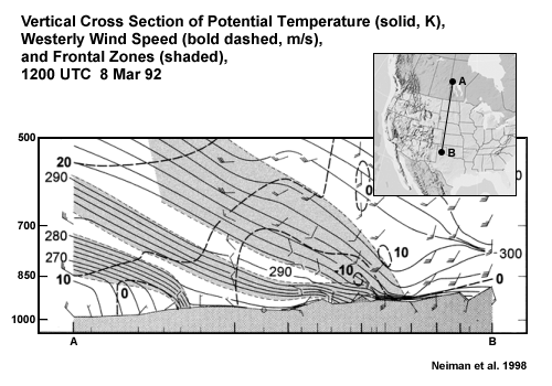
As with occlusion, the outcome of frontal merger is the displacement of relatively warm air upward and the creation of clouds and precipitation. To determine the occurrence of frontal merger, closely examine cross sections, such as the one shown here. Regions of frontal merger are most likely to experience mesoscale bands of precipitation.
Frontal merger does not conveniently fit with any cyclone model. However, cyclones may play a role in the formation of the fronts involved. On a synoptic scale, this process will most likely occur when an arctic outbreak from high latitudes encounters either a stationary front or a warm front at lower latitudes. Thus, the interaction of synoptic systems can enhance vertical motion in a linear pattern. In a moist environment, this can lead to mesoscale precipitation bands.
Dominant Mesoscale Banding Processes » CSI and Slantwise Convection
Dominant Mesoscale Banding Processes » CSI and Slantwise Convection » Introduction
Precipitation bands frequently occur in the absence of a frontal structure. When these bands appear in a stable environment, in the absence of upright convection or other known forcing mechanisms, we may be dealing with slantwise convection.
Slantwise convection may account for bands that appear in the midst of a broad precipitation shield or for nearly all of the precipitation in a single event. The great importance of slantwise convection lies in the fact that it produces significant, sometimes unanticipated, banded precipitation.
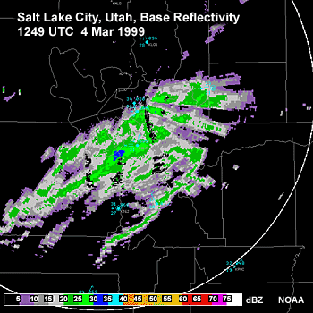
The precipitation bands associated with slantwise convection can be from 100 to more than 500 km long and from 5 to 40 km wide. This radar image shows banded precipitation near Salt Lake City, Utah on 4 March 1999. The bands go right across the mountain ranges, which can be seen as areas where the echo was removed due to ground clutter. Most of the accumulation from this storm came from these of bands.
Dominant Mesoscale Banding Processes » CSI and Slantwise Convection » CSI and Stability
Slantwise convection results from the release of conditional symmetric instability (CSI). CSI is not easy to visualize. Basically, the idea is that an air parcel may be stable with respect to vertical displacement (convective stability), and it may be stable with respect to horizontal displacement (inertial stability), but it can be unstable when it ascends along a slantwise path. This is why CSI is sometimes called slantwise convection.

But what does it mean to be stable? First let's look at vertical stability. When a dry parcel of air is displaced vertically, it cools at the adiabatic lapse rate of about 10°C/km [animate]. If the surrounding air is cooler yet, that parcel becomes warmer and less dense than its surroundings and will rise convectively. This environment is absolutely unstable, which is quite uncommon. When a saturated parcel of air is displaced vertically, it cools more slowly, at the moist adiabatic lapse rate of about 6.5°C/km. If it still is warmer than its environment, it will continue to rise convectively. If the environment is stable with respect to dry ascent, but not moist ascent, then it is conditionally unstable. If the environment is stable with respect to moist ascent, then it is absolutely stable.
Dominant Mesoscale Banding Processes » CSI and Slantwise Convection » Horizontal Stability

Horizontal stability arises from inertial stability. Flow with positive inertial stability follows isobars or height contours. CSI requires weak inertial stability, so that flow can deviate horizontally from following heights or isobars as it ascends. Let's see how that occurs.
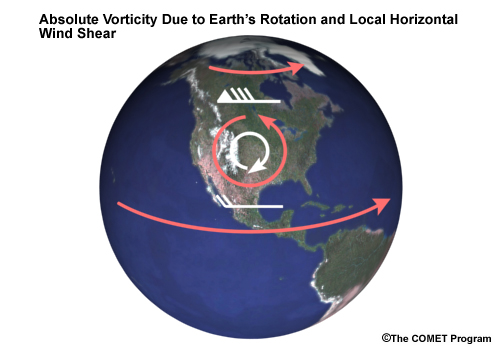
Inertial stability is determined by the absolute vorticity. When absolute vorticity is negative, the atmosphere is inertially unstable. Absolute vorticity is the sum of the earth's vorticity and the relative vorticity. The earth's vorticity is a cyclonic vorticity caused by the earth's rotation, as shown here.
A strong, anticyclonic relative vorticity may counteract the earth's cyclonic vorticity, resulting in a weak absolute vorticity. Weak absolute vorticity leads to weak inertial stability.
Anticyclonic vorticity may arise in two ways. The first is when flow bends in an anticyclonic fashion, as shown here.
A second factor contributing to anticyclonic vorticity may be horizontal wind shear. Typically, this is found on the equator side of a jet, as illustrated here.
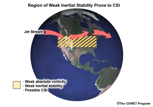
CSI occurs under conditions of weak or neutral inertial and convective stability. If we position ourselves on the equator side of a jet, then that flow generates an anticyclonic relative vorticity. This is the area where we may find weak inertial stabilitythe area most prone to CSI.
Dominant Mesoscale Banding Processes » CSI and Slantwise Convection » Question
Question 25
Use the pull-down menu to (choose the best answer.)
The correct answers are highlighted above.
It is true that the earth's vorticity is always cyclonic, even in the southern hemisphere and absolute vorticity is weak when relative vorticity is strongly anticyclonic.
Dominant Mesoscale Banding Processes » CSI and Slantwise Convection » Assessing CSI
To review, a parcel may be stable with respect to vertical displacement (convective stability) and the parcel may be stable with respect to horizontal displacement (inertial stability), but the parcel can be unstable when it ascends a slantwise path.
One way to assess CSI is with a vertical cross section drawn perpendicular to the mean wind shear. On this cross section we plot equivalent potential temperature, known as theta-e, and geostrophic momentum. Under conditions of weak or neutral inertial and convective stability, when we lift an air parcel, it follows a surface of constant momentum. If that path takes the parcel to a lower equivalent potential temperature, then the advected air parcel becomes warmer than its environment. The parcel then continues to rise convectively along the slanted path, and we get slantwise convection. Thus, in this cross section, CSI occurs where the contours of equivalent potential temperature become steeper than the momentum contours. Slantwise convection would result in bands oriented parallel to the flow and perpendicular to the cross section.
There are several caveats here, but the most important one is that if the environment is unstable with respect to vertical convection, then that process will dominate. In a cross section, vertical convection would occur anyplace where theta-e decreases with height. This includes locations where the contours of equivalent potential temperature are overturned past vertical.
Also note that some initial ascent is required to release CSI. Without that initial trigger, CSI is not released and slantwise convection does not occur.
Dominant Mesoscale Banding Processes » CSI and Slantwise Convection » Question
Question 26
When assessing CSI, a vertical cross section is drawn _____ to the flow. (Choose the best answer.)
The correct answer is b).
The cross section is drawn perpendicular to both the flow and the thickness contours.
Dominant Mesoscale Banding Processes » CSI and Slantwise Convection » Visualizing CSI
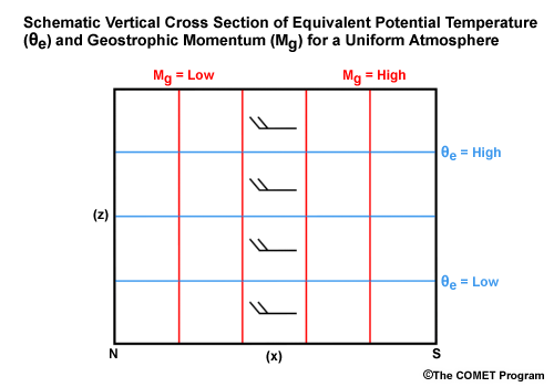
Under what conditions will contours of equivalent potential temperature become steeper than the contours of momentum? This conceptual vertical cross section depicts a relatively uniform thermal environment with weak conditional stability and flow into the page. The atmospheric lapse rate would be slightly less than the moist adiabatic lapse rate. On a cross section, contours of equivalent potential temperature would be horizontal and spaced far apart. Under these conditions, rising air could never move from higher to lower equivalent potential temperature.
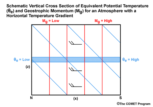
In order to achieve CSI, we first need to tilt the lines of equivalent potential temperature, so that the atmosphere is cooler to the left. Thus, the first thing we need with CSI is a horizontal temperature gradient.
Under conditions of weak conditional stability, there is only a small vertical gradient in equivalent potential temperature. Thus we require only a relatively small horizontal temperature gradient to tilt the contours steeply over a substantial depth. With a more stable environment, the same horizontal temperature gradient would result in very little tilt.
In our cross section depicting a uniform atmospheric environment, momentum contours would be essentially vertical. Remember, reduced to its most simplistic terms, momentum is just mass times the velocity. On this cross section, momentum increases from left to right as an artifact of how we compute geostrophic momentum, but what we really care about is the orientation of the contours.
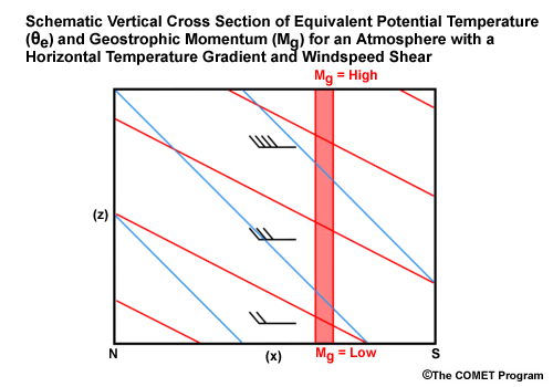
Now let's add strong wind speed shear into the line of the cross section so that momentum increases as we ascend. This tilts the momentum surfaces over to the left, causing momentum to increase with height in any given vertical profile.
We see that contours of equivalent potential temperature can become steeper than momentum surfaces if we satisfy two conditions:
- A horizontal gradient in equivalent potential temperature
- A strong vertical gradient in geostrophic momentum
Thus, CSI may form in an environment with
- Weak conditional stability
- A horizontal temperature gradient
- Strong unidirectional wind shear
Dominant Mesoscale Banding Processes » CSI and Slantwise Convection » Question
Question 27
In the absence of strong wind shear, momentum surfaces have a _____ slope. (Choose the best answer.)
The correct answer is b).
In the absence of appreciable wind shear, momentum surfaces are nearly vertical.
Dominant Mesoscale Banding Processes » CSI and Slantwise Convection » Question
Question 28
Steeply sloping contours of equivalent potential temperature typically occur with which of the following conditions? (Choose all that apply.)
The correct answers are a) and c).
A horizontal temperature gradient tilts the contours of equivalent potential temperature (theta-e). The tilt becomes steep in the presence of weak vertical stability.
Dominant Mesoscale Banding Processes » CSI and Slantwise Convection » Favorable Conditions
Before CSI contributes to banded precipitation, we need to add two crucial ingredients: moisture and lift. For moisture, we require a relatively saturated atmosphere with relative humidity over 80%. For lift, consult model products such as vertical velocity or omega that indicate rising motions required to initiate the release of CSI. Because CSI requires horizontal temperature gradients, it frequently occurs in association with frontogenesis, which may provide the initial ascent.
Question 29
On the image below:
- Use the pen to mark the temperature profile where you might expect to find CSI.
When you have finished, select Done.
Compare your answer to the answer below.
Please continue watching the video above.
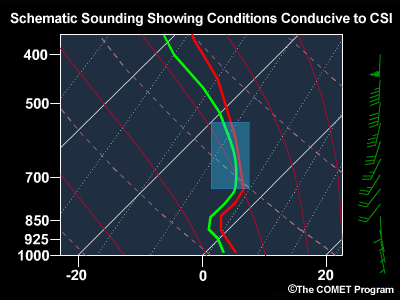
In this cross section, you would look for CSI in the range from about 750 up to about 550 hPa. This part of the atmosphere shows weak conditional stability, high relative humidity, and winds increasing from 20 to 40 knots.
While these conditions do not constitute an assessment of CSI, methods using cross sectional analysis can be used to directly assess the conditions. See the In Depth section for a step-by-step approach for assessing CSI.
Dominant Mesoscale Banding Processes » CSI and Slantwise Convection » Synoptic Setting
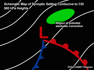
Generally, the conditions for CSI are met in areas associated with a shallow front. These can be either ahead of a warm front or behind an anafront. These regions are usually characterized by a convectively stable environment and conditions that are near saturation. Another typical feature is the presence of a jet just north of the area. This provides the anticyclonic relative vorticity that is typical of regions of low inertial stability. The jet also contributes to the strong vertical shear found in CSI events.
Dominant Mesoscale Banding Processes » CSI and Slantwise Convection » Question
Question 30
CSI can occur without slantwise convection, but slantwise convection cannot occur without CSI. (Choose the best answer.)
The correct answer is True.
Slantwise convection occurs when CSI is released. However, the release of CSI requires some initial ascent. So it is possible for unreleased CSI to occur, without slantwise convection.
Dominant Mesoscale Banding Processes » CSI and Slantwise Convection » Summary
In summary, a few simple rules will help you be aware of the potential for CSI and mesoscale banding associated with it.
- CSI occurs in regions of thermal gradients, which may or may not be frontal zones.
- CSI occurs in moist environments, near saturation.
- CSI occurs under conditions of strong vertical wind speed shear, commonly unidirectional.
- CSI occurs under conditions of weak stability.
- CSI occurs under conditions of weak inertial stability, indicated by small absolute vorticity.
- CSI typically occurs in the middle levels of the atmosphere, frequently above orographic influences.
See the In Depth section for a detailed look at one method for forecasting CSI and slantwise convection.
To learn more, also see the COMET Webcast:
Slantwise Convection: An Operational Approach (https://www.meted.ucar.edu/norlat/slant/)
Dominant Mesoscale Banding Processes » Case Example
Dominant Mesoscale Banding Processes » Case Example » Introduction
During the early morning hours of 4 March 1999 a small, but unexpected snow event took place along the Wasatch Front and adjacent mountains. Snowfall totals of 1-2 inches were common along the valleys and benches with up to 6 inches in the mountain valleys and ski areas.
On average two to three CSI events occur in northern Utah per winter. CSI-induced bands will nearly always concentrate precipitation and produce intensities and amounts much greater than what the general synoptic pattern would suggest is possible.
This short case exercise will examine the March 1999 event, which was reported by Dunn in 1999.
Dominant Mesoscale Banding Processes » Case Example » Synoptic Setting
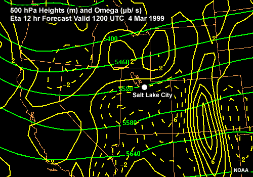
From a synoptic viewpoint, at 1200 UTC on 4 March, the 500 hPa Eta 12 hour forecast showed generally zonal, low-amplitude flow across the West with a few weak embedded waves. In the northern Utah region, the height gradient at 500 hPa increased slightly to the north and the omega field showed an area of weak upward motion covering most of Utah.
Question 31
Based on this plot of 500 hPa heights and vertical velocity, what indicators are consistent with a forecast of banded precipitation near Salt Lake City, Utah due to slantwise convection? (Choose all that apply.)
The correct answers are c) and e).
Please continue watching the video above.
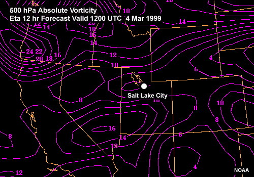
The Salt Lake City area was in flow that was weakly anticyclonic at 500 hPa, which would lead to weak inertial stability, consistent with CSI. In fact, this 12 hour forecast of absolute vorticity shows a minimum just south of Great Salt Lake, where the banded precipitation occurred. Furthermore, the negative omega values across Utah could have provided the initial ascent required to release CSI via slantwise convection.
Dominant Mesoscale Banding Processes » Case Example » Sounding
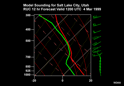
Question 32
What do you see in this sounding from Salt Lake City that is consistent with CSI and slantwise convection? (Choose all that apply.)
The correct answers are a), b) and d).
The Salt Lake City sounding at 1200 UTC revealed strong vertical wind shear in the midlevels, with 15 knots at 700 hPa increasing to 50 knots at 500 hPa. Also note the moist layer with weak stability from about 500-650 hPa. Thus, from the sounding and the previous 500 hPa plot, we see that the general criteria for CSI appear to be satisfied. Let's plot cross sections to see where the CSI occurs.
Dominant Mesoscale Banding Processes » Case Example » Cross Sections
Question 33
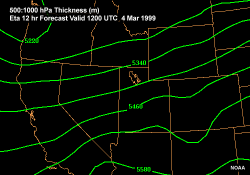
On this plot of 500-1000 hPa thickness, which line would be most appropriate for evaluating CSI? (Choose the best answer.)
The correct answer is a) A - A'.
It is oriented perpendicular to the thickness contours.
Question 34
On this cross section, we have plotted two fields:
- Geostrophic momentum (Mg)
- Equivalent potential temperature (theta-e)
On the image below:
- Use the pen to outline the region of CSI.
When you have finished, select Done.
Compare your answer to the answer below.

We have shaded the area where theta-e contours have a steeper slope than Mg contours. Remember that if theta-e decreases with height, there is convective instability and upright convection will dominate. That does not occur in this event. So, we have CSI, but not convective instability. Now let's determine where the CSI likely resulted in slantwise convection.
Question 35
We have added relative humidity to the cross section.
On the image below:
- Use the pen to outline the region that satisfies all the criteria for slantwise convection.
When you have finished, select Done.
Compare your answer to the answer below.
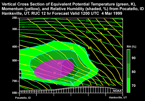
The shaded region has all of the necessary ingredients for slantwise convection:
- CSI, as shown in the theta-e and momentum fields
- A relative humidity of 80%, which is at or near saturation with respect to ice
And remember, we saw in a previous plot that most of the area was under the influence of weak ascent. This provided the ascent necessary for cooling and condensation, which initiated the release of CSI via slantwise convection.
Dominant Mesoscale Banding Processes » Questions
Dominant Mesoscale Banding Processes » Questions » Question
Question 36
Use the pull-down menu to (choose the best answer.)
The correct answers are highlighted above.
When horizontal temperature gradients weaken (negative frontogenesis) we term it frontolysis.
Dominant Mesoscale Banding Processes » Questions » Question
Question 37
Use the pull-down menu to (choose the best answer.)
The correct answers are highlighted above.
The ageostrophic circulation acts to weaken the horizontal temperature gradient. Thus, we see ascent and cooling on the warm side of the front and descent and warming on the cool side.
Dominant Mesoscale Banding Processes » Questions » Question
Question 38
Frontogenesis may result from which of the following processes? (Choose all that apply.)
The correct answers are a), b), and c).
Deformation compresses temperature gradients through warm and cold air advection. Melting and/or evaporation cool air on the cool side of a frontal zone, increasing the temperature gradient. Frontal merger combines two or more frontal zones, which increases the temperature gradient. CSI on the other hand, benefits from frontogenesis as a horizontal temperature gradient is required to generate CSI.
Dominant Mesoscale Banding Processes » Questions » Question
Question 39
How does frontal merger differ from frontal occlusion? (Choose the best answer.)
The correct answer is a).
The distinction is important because a frontal occlusion can result in a trowal situation while frontal merger will not. However, frontal merger can result in strong frontogenesis and heavy banded precipitation near the merged front.
Dominant Mesoscale Banding Processes » Questions » Question
Question 40
Once the lower atmosphere is saturated, falling precipitation will no longer contribute to cooling. (Choose the best answer.)
The correct answer is False.
Even a saturated atmosphere can cool. Melting of frozen precipitation will also cool the air, though not as effectively as evaporation.
Dominant Mesoscale Banding Processes » Questions » Question
Question 41
Use the pull-down menu to (choose the best answer.)
The correct answers are highlighted above.
Temperature gradients will strengthen when you warm the air on the warm side of a frontal zone, cool the air on the cool side of a frontal zone, or both. Cooling the air on the warm side of a frontal zone will either advance the front or possibly Weaken the horizontal temperature gradient (frontolysis).
Model Representations of Banded Precipitation
At the end of this section you should be able to do the following things:
- Given the grid spacing determine the grid resolution
- Describe the characteristics of a hydrostatic atmosphere
- State why high-resolution NWP models need to be non-hydrostatic
- Describe the need for parameterization in NWP models
- Describe the pros and cons of parameterization versus explicit treatment of processes
- Describe the difference between prognostic and diagnostic moisture physics, and the benefits of each
- Characterize COAMPS and NOGAPS
Model Representations of Banded Precipitation » Factors
Model Representations of Banded Precipitation » Factors » Introduction
Precipitation bands occur in various widths. They range from the meso-alpha rain shield ahead of a classic warm front, hundreds of kilometers wide, to the meso-gamma line of convective rain shafts of a classic supercell thunderstorm, 1 to 2 km wide. Yet, our present numerical modeling prowess allows an accurate portrayal only of the former, meso-alpha band.
The reasons for this failure are varied. Under the best of conditions NWP models may struggle to produce an accurate precipitation forecast. In fact, NWP models typically show the least skill at quantitative precipitation forecasts. When confronted with processes that operate on small spatial and time scales, models may fail to forecast any precipitation at all. This section will examine some of the reasons that limit the ability of NWP models to forecast mesoscale banded precipitation.
The following discussion assumes that you already have some familiarity with mesoscale NWP models. For a brief review of mesoscale models, see the COMET module How Mesoscale Models Work.
How Mesoscale Models Work (https://www.meted.ucar.edu/mesoprim/models/)
Model Representations of Banded Precipitation » Factors » Resolution - Grid Spacing vs. Grid Resolution
The primary reason that our present NWP models fail to predict meso-gamma precipitation bands is that the bands are so small that the models simply cannot clearly produce them.
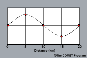
Consider a model that uses a grid spacing of 5 km. This means that the model looks at the atmosphere every 5 km. In numerical modeling, 5 grid points (4 grid spaces) are generally accepted as a minimum to resolve a given wave although more are always helpful. Thus, the smallest wave that our model will be able to simulate is 20 km long. This is the models minimum grid resolution. Our 5 km model will not produce waves smaller than this value.
The lesson here is that you cannot expect to see a 15 km wide band of precipitation in a model forecast produced with an operational 15 km grid spacing. The most narrow you could reasonably expect would be 60 km.
Model Representations of Banded Precipitation » Factors » Representing Convection: Introduction
Although convection is addressed in many other sources, there is no other atmospheric phenomenon that is of such small horizontal dimension and yet spans the depth of the troposphere while providing NWP models and modelers with the challenges of:
- Rapid cloud development
- Precipitation generation (including hail)
- Incoming shortwave and upwelling longwave radiation
- Violent upward and downward motions
- Turbulence generated by strong, small-scale vertical motions.
Furthermore, mesoscale banded precipitation frequently results from convective precipitation embedded within a larger precipitation field. For these reasons, if a model can adequately depict convection, we can be reasonably certain that it will adequately depict mesoscale banded precipitation related to midlatitude cyclones.
Model Representations of Banded Precipitation » Factors » Hydrostatic vs. Non-Hydrostatic
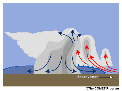
A hydrostatic atmosphere implies that vertical motions are insignificant. Air parcels move great horizontal distances without rising or sinking. However, the convective environment is one of powerful updrafts and downdrafts; we term such an environment non-hydrostatic. Thus, non-hydrostatic NWP models allow strong vertical motions. Current models with grid spacings of 10 km or less treat the atmosphere non-hydrostatically. In fact, most mesoscale NWP models are now non-hydrostatic, including COAMPS and the AFWA MM5.
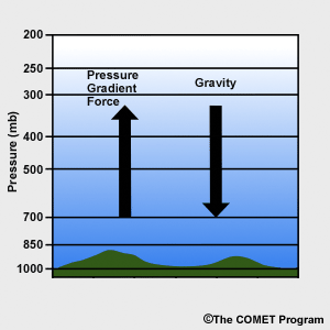
When the atmosphere is in hydrostatic equilibrium, the downward weight of the atmosphere balances the upward-directed pressure gradient force. An assumption of hydrostatic equilibrium is valid for synoptic- and global-scale systems and for some mesoscale phenomena. Non-hydrostatic processes and their effects become important when the length of a feature is approximately equal to its height. Since the heights of most weather phenomena are limited by the height of the troposphere, this becomes an issue for features approximately 10 km and less in size. Important weather examples with significant non-hydrostatic processes include convective storms, gust fronts and other convergence lines, and gravity waves, including mountain waves and turbulence.
Model Representations of Banded Precipitation » Factors » Explicit Cloud vs. Cumulus Parameterization
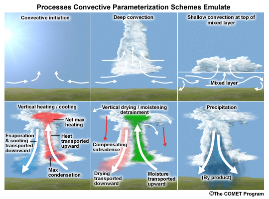
This graphic depicts some of the process that must be accounted for over the life cycle of a single convective cell. High-resolution models that treat the atmosphere non-hydrostatically will ideally be able to simulate these processes. To look at clouds in this painstaking detail is to treat them explicitly in a model. However, a model with wide grid spacing cannot treat clouds with such care since the model grid is too widely spaced to see each individual thunderstorm. Yet we cant afford to ignore the convection altogether. So what do we do? The answer is cumulus parameterization.
Clearly, dealing with convective clouds explicitly is superior to cumulus parameterization. However, an explicit approach to cloud modeling takes far more computational time than most cumulus parameterization schemes. In short, cumulus parameterization is expedient, but cannot resolve individual convective clouds, only the aggregate changes in temperature and moisture that they provide. As a result, parameterization is better suited to models with wider grid spacing (> 25 km). Explicit representation of convection can be very detailed, but such insight only comes at the expense of a great deal of computing power and time. Thus, explicit cloud treatment is more appropriate for models of a finer grid spacing (< 10 km).
Model Representations of Banded Precipitation » Factors » Representation of Precipitation Processes
The representation of precipitation processes is of particular importance to our larger discussion of mesoscale banded precipitation, as well as our specific example of convection.
NWP models treat precipitation with either diagnostic or prognostic moisture physics. With diagnostic moisture physics, the model checks each grid point from the top down to determine if the atmosphere is supersaturated (relative humidity > 100%). If it is, the excess moisture is carried to the next lowest level in the model. This moisture is accumulated until it reaches the ground.
With prognostic moisture physics, the model has separate equations that account for rain production, ice crystal production, and even hail generation. These equations examine variables such as temperature and wind velocity in addition to excess moisture at different levels for each grid point.
The more elaborate prognostic moisture physics will generally produce a better forecast, but requires more computational work than diagnostic moisture physics. And remember, regardless of the moisture physics, NWP models still struggle to produce accurate quantitative precipitation forecasts.
Model Representations of Banded Precipitation » Factors » Interaction of Convection with Ambient Environment
Whether modeling with a cumulus parameterization scheme or an explicit treatment for convection, it is important to recognize that such small-scale features may well have an impact on meteorological features of larger scales. If a thunderstorm occurs on a grid column in your model, then that column has become warmer and more moist through a much deeper layer than it had been previously. While the changes in moisture are important, the changes in temperature are crucial to having a realistic simulation. Having a large area of thunderstorm activity means a broad area of deep convective heating. This heating can alter flow in the upper troposphere and may impact the jet stream.
Thus, a mesoscale model that accurately depicts convection (or other mesoscale phenomena) may also produce a better synoptic forecast.
Model Representations of Banded Precipitation » Factors » Conclusions
There is an almost bewildering array of models available to forecasters, both at home and abroad. Each model has its strengths and weaknesses. Depending on the model resolution and physics, some may be better suited than others for a particular event that might include bands of heavy precipitation.
So, good forecasting requires that you:
- Have a good situational awareness of the synoptic situation,
- Have a good awareness of the climatology of your particular area of responsibility,
- Examine the model analysis to see how well the current model run initialized, and
- Are familiar with model characteristics.
Model characteristics may be compared by going to the Operational Models Matrix: Characteristics of Operational NWP Models.
To compare the characteristics of different NWP models, see the Operational Models Matrix (https://sites.google.com/ucar.edu/operational-models-encyclo/home)
Model Representations of Banded Precipitation » Questions
Model Representations of Banded Precipitation » Questions » Question
Question 42
If a model can adequately depict convection, we can be reasonably certain that it will adequately depict mesoscale banded precipitation related to midlatitude cyclones. (Choose the best answer.)
The correct answer is True.
Most of the processes related to the formation of banded precipitation also occur with convection, including rapid ascent and high spatial and temporal variability. Thus, a model capable of depicting convection should be able to depict banded precipitation.
Model Representations of Banded Precipitation » Questions » Question
Question 43
Greater grid spacing results in greater resolution. (Choose the best answer.)
The correct answer is False.
Model resolution increases as grid spacing decreases.
Model Representations of Banded Precipitation » Questions » Question
Question 44
As grid spacing decreases in NWP models, it becomes more important to treat the atmosphere non-hydrostatically. (Choose the best answer.)
The correct answer is True.
A non-hydrostatic environment allows large vertical motions over short horizontal distances. As grid spacing decreases it becomes important for models to simulate these motions.
Model Representations of Banded Precipitation » Questions » Question
Question 45
Cumulus parameterization is better suited to models with larger grid spacing (› 25 km). (Choose the best answer.)
The correct answer is True.
As grid spacing decreases, models become more likely to treat convection explicitly, rather than with parameterization.
Model Representations of Banded Precipitation » Missouri, 10 December 2003
Model Representations of Banded Precipitation » Missouri, 10 December 2003 » Introduction
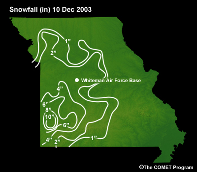
On 10 December 2003, banded heavy snow fell over portions of Missouri in the vicinity of Whiteman Air Force Base. While snow totals there were only about 1 inch, there were locations less than 100 km away from Whiteman with accumulations as high as 5 inches, as shown in this figure.
As a forecaster early on 10 December 2003, your task would have been to determine if banded heavy snowfall would occur, and if so, whether or not those bands would affect Whiteman.
Model output from both the COAMPS and the NOGAPS models are examined for this exercise. As you know, the COAMPS is a higher-resolution, non-hydrostatic model (grid points every 27 km) while the NOGAPS has a coarser-resolution, hydrostatic architecture (grid points every 1.0° x 1.0°, about 100 km). While the COAMPS should permit us to see finer-scale features, it also deals with convection directly. However, it is crucial to note that the precipitation fields shown here are 6 hour accumulations. As such, there may be smaller bands that occur during a given integration that are masked by the bands very motion. At the end of 6 hours the smaller band may have propagated some distance, and its impact during any shorter period during those 6 hours may be lost or at least diminished. The meso-alpha structure of a precipitation field is retained, but smaller features are not revealed.
Model Representations of Banded Precipitation » Missouri, 10 December 2003 » Synoptic Setting - 500 hPa

At 0000 UTC 10 December 2003, as analyzed by the NOGAPS model, a vigorous cutoff low was tracking across Oklahoma and moving east-northeastward toward southern Missouri.
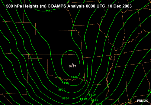
The COAMPS model analysis at this time depicted a slightly stronger, sharper trough centered over eastern Oklahoma. Compared to the NOGAPS analysis, the cutoff center is slightly deeper and located a bit farther to the southeast. (Note that the contour interval is halved in the COAMPS analysis.)
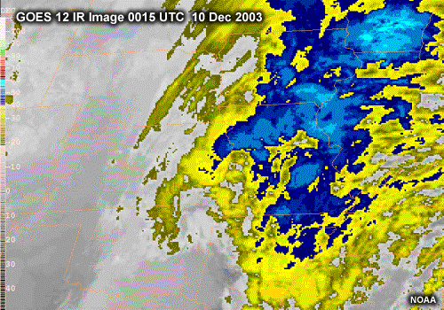
The storm system aloft was clearly defined in the infrared satellite imagery at that time, with a comma-shaped signature centered over northeastern Oklahoma and widespread deep cloudiness out ahead of the system.
Model Representations of Banded Precipitation » Missouri, 10 December 2003 » Synoptic Setting - Surface
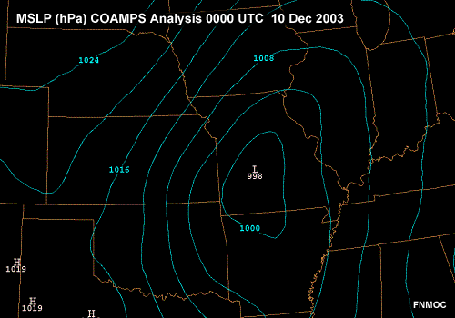
This deep trough aloft had caused a strong surface low pressure system to form out ahead of the 500 hPa trough, centered over central Missouri.
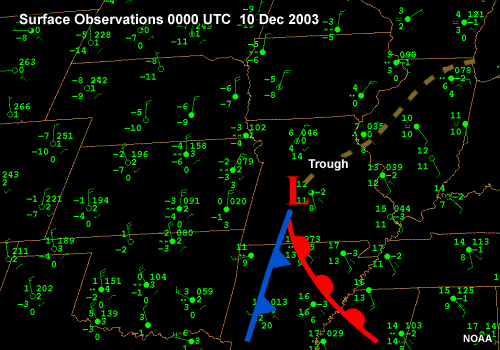
The surface trough was becoming somewhat elongated at this time, with cyclonic flow extending all the way up past the Great Lakes and southwestward into Texas. Also note the extended fetch of northerly flow from the northern plains to eastern Oklahoma. The associated cold front extended from the surface low south-southeastward through Arkansas into eastern Louisiana.
Model Representations of Banded Precipitation » Missouri, 10 December 2003 » Moisture and Ascent
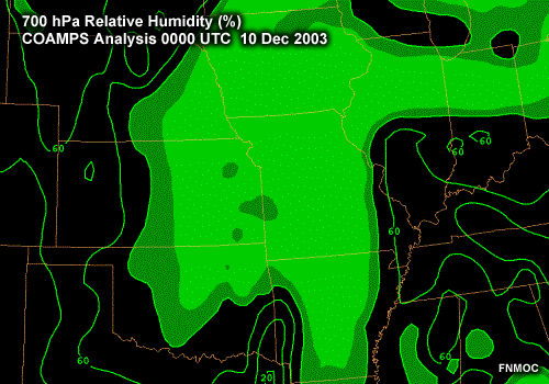
Aside from moist conditions over the cold frontal zone, high relative humidity values at 700 hPa were confined to regions north and northeast of the upper low and also well out in front of the cold front over the southeastern U.S..
The COAMPS analysis indicated a well-defined dry intrusion aloft, the dry conveyor belt, over extreme southeast Oklahoma and northeastern Texas. This dry conveyor was moving northward into western Arkansas toward the Missouri border.
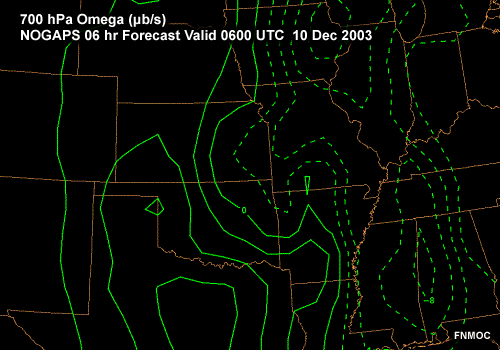
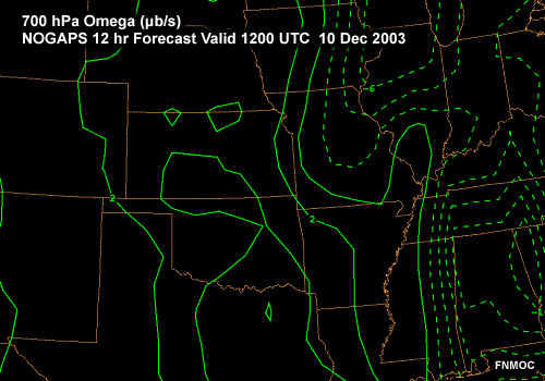
At 6 and 12 hours of simulation in the NOGAPS model, an area of moderate upward motion, was forecast to track across central and northeastern Missouri. The rising motions formed in response to the approach of the strong upper trough.
Model Representations of Banded Precipitation » Missouri, 10 December 2003 » Frontogenesis and Precipitation - NOGAPS
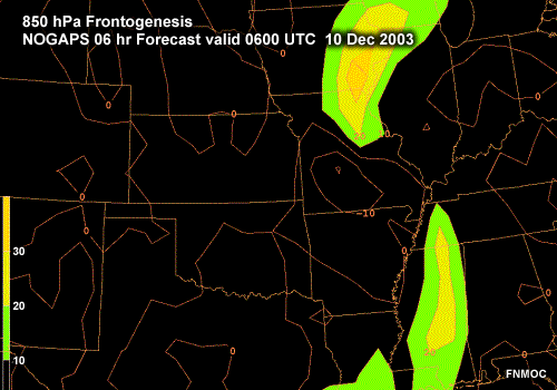
At 0600 UTC 10 December, NOGAPS was predicting regions of significant frontogenesis at 850 hPa over northeastern Missouri and near the pre-existing surface cold front over Mississippi.
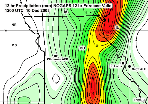
The coarse NOGAPS solution reveals one large, meso-alpha band of precipitation extending from the Illinois/Iowa border down to south-central Missouri. Over 0.75 inch (19 mm) of liquid precipitation (or its equivalent) was predicted by NOGAPS in 6 hours over a broad area. A smaller area of weaker precipitation is predicted along the Oklahoma-Kansas border; a banded structure there is not obvious.
Model Representations of Banded Precipitation » Missouri, 10 December 2003 » Frontogenesis and Precipitation - COAMPS
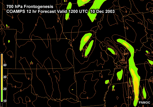
The 12 hour forecast of 700 hPa frontogenesis by COAMPS revealed significant positive values associated with the cold front over western Tennessee into northern Alabama and also over central and north-central Missouri. It appears that this forcing may have played a role in the development of model precipitation over central Missouri.
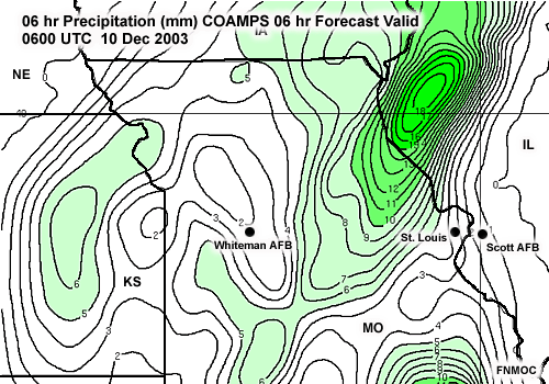
The finer COAMPS solution depicts several bands for the same period. The first originates in largely the same region as shown by NOGAPS, near northeast Missouri, but angling more southwestward toward southwest Missouri. A second band is shown over extreme northeastern Arkansas, while a third area with more of a banded shape is shown over eastern Kansas. In all, COAMPS forecasts three bands, as opposed to the single large band forecast by NOGAPS.
Model Representations of Banded Precipitation » Missouri, 10 December 2003 » Warm Conveyor / Trowal
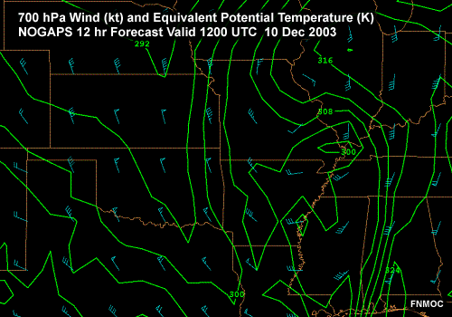
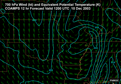
Closer examination of the NOGAPS and COAMPS predictions in this case reveal some similarities to a case discussed earlier in this module, the well-developed trowal of 10 November 1998. Precipitation bands developed west and northwest of the upper cutoff low in both cases.
Shown here are the 12 hour, 700 hPa wind and theta-e predictions at 1200 UTC on 10 December 2003.
In both cases, warm air aloft is being wrapped in a counterclockwise direction back around the upper low, as part of a relatively moderate warm conveyor belt or trowal situation, as discussed previously. Many previous studies have shown that this airflow continues to ascend on the backside of the storm system, thereby contributing to development of a precipitation band. In both models, significant precipitation was predicted to develop over central and northeastern Missouri, which coincides with the ascending, wraparound motion of the warm air aloft.
Model Representations of Banded Precipitation » Missouri, 10 December 2003 » Verification
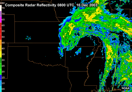
This composite radar image was observed at 0800 UTC on 10 December. Note the precipitation band in central Missouri, northwest of the cutoff low. More precipitation fell over southwestern Missouri than either model predicted. NOGAPS seemed to have a better handle on the southern portion of the precipitating region although this models secondary precipitation max was located well to the east of the observed max.
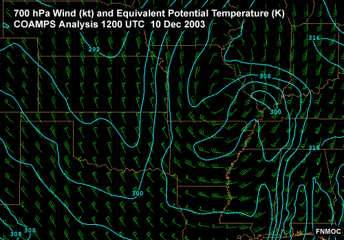
When one takes a look at the COAMPS analyzed fields at 700 hPa for 1200 UTC 10 December, some errors in the 12 hour forecast for this time are apparent. The wraparound moisture in the analysis extends into southwestern Missouri, farther south and west than in the forecast. Moreover, the winds wrapping around the storm aloft are about 10 to 15 knots stronger than those in the forecast, indicating that COAMPS underpredicted the strength and extent of the wraparound of the warm conveyor belt. This was likely the primary cause of COAMPSs severe underprediction of precipitation amounts over southwestern Missouri. The ascending warm conveyor apparently ended up slightly stronger and displaced compared to the NOGAPS and COAMPS predictions.
What do we make of all of this? It would appear that elements of the truth are found in both models solutions. Indeed, a dominant band of precipitation is present in the radar observations, as suggested by the NOGAPS solutions. Concurrently, additional bands were forming, a solution hinted at in the COAMPS values.
Model Representations of Banded Precipitation » Missouri, 10 December 2003 » Conclusions
In summary, neither model handled the actual weather perfectly. As with most numerical models, the final solutions are based in part on initial conditions (the observations) that do not resolve every detail. NOGAPS has a coarser grid spacing than COAMPS and uses special parameterization schemes for convection and other processes. Moreover, such schemes are often tuned to work within a particular model architecture. As a consequence, in this case the placement and accumulations of the major band are handled better by NOGAPS. By contrast, the non-hydrostatic, cumulus-resolving COAMPS solution portends the presence of bands, although they are not well placed or indicate the correct intensity. Yet, when we consider that so many precipitation bands are convective, the need for non-hydrostatic models and their continued development becomes clear. In the end, the messages from both models were worthwhile and clear: Precipitation bands near St. Louis were likely, but accumulations would not be significant.
Satellite Detection of Banded Precipitation
At the end of this section you should be able to do the following things:
- Describe the benefits and drawbacks of satellite estimates of precipitation
- Recall at least 4 satellite sensors that measure precipitation
- Describe the benefits and drawbacks of the GOES Precipitation Index
- Describe the benefits and drawbacks of precipitation estimates derived from microwave sensors
- Describe how a blended precipitation product is derived
Satellite Detection of Banded Precipitation » Discussion
Satellite Detection of Banded Precipitation » Discussion » Introduction
In most parts of the world, Doppler radar data are not available. However, satellites can frequently detect banded precipitation. This section provides an overview of the different satellites and sensors used to detect and estimate precipitation. We will examine Hurricane Jeanne, as it came ashore in the southeast U.S. to provide a basis of comparison.
Satellite Detection of Banded Precipitation » Discussion » IR
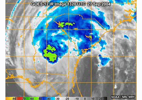
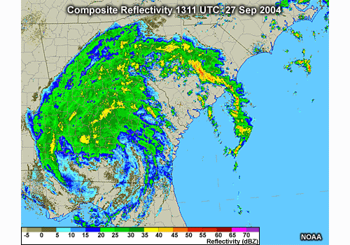
Infrared (IR) emissions are most useful for estimating precipitation from convective clouds because higher, and thus colder, cloud tops correlate with higher precipitation rates. In this method of estimating precipitation, IR temperatures are averaged over various areas and times. Those averages are then compared with precipitation measurements to arrive at an operational temperature-precipitation correlation. One example of this is the GOES Precipitation Index, or GPI. It uses 235 kelvins as the IR temperature with the best correlation to average precipitation for areas spanning 50-250 km over 3-24 hours.
These images compare a GOES IR image with a composite radar image for Hurricane Jeanne as it moved over Georgia. One can see that the IR image fails to provide the same resolution as the radar image. When averaged over longer periods of time, the resolution drops even further. Thus, the GOES precipitation index provides us with a general overview of precipitation, but fails to depict most mesoscale banding.
Other disadvantages of IR-only techniques are the lack of detection of rain from warm clouds, the inability to differentiate between convective precipitation and cold cirrus, and unreliable results in midlatitude regions during the colder seasons. There is also a tendency to underestimate precipitation early in the lifecycle of convective systems and to overestimate precipitation in the dissipating stages.
The primary advantage of IR-based techniques is the high frequency of images: 30 min or less for geostationary satellites. Recent satellite precipitation estimates have combined low-earth orbiting microwave measurements, which have high resolution, but low frequency, with the more frequently available geostationary IR. At the end of this section, we will examine the blended precipitation product developed by the Naval Research Laboratory in Monterey.
Satellite Detection of Banded Precipitation » Discussion » Special Sensor Microwave Imager (SSM/I)
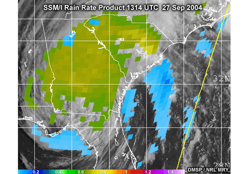
The Defense Meteorological Satellite Program (DMSP) Special Sensor Microwave/Imager (SSM/I) brought fundamental change to the identification of precipitation from satellites because it directly detects precipitation in clouds. These images show the SSM/I-derived rain rate along with the composite radar reflectivity for Hurricane Jeanne over Georgia. Note that the major precipitation band on the northwest side of the storm is preserved in the satellite image, though its fine structure is lost.
The SSM/I measures the microwave scattering and emission signatures of hydrometeors. The brightness temperatures at 37 and 85 GHz are used to infer the quantity of liquid water and ice in a column, which correlates well to surface precipitation. The 85 GHz channel is strongly scattered by ice and is used to define rain intensity.
Both scattering and emission-based methods are used to identify rainfall. Emission techniques work well over the ocean where the background emissivity from the ocean surface is low and uniform. Over land, the background emissivity is higher and more variable, making it difficult to distinguish raindrops. Therefore, rain-retrievals over land rely upon a measure of scattering.
Liquid or solid water particles that are suspended in the air. Particles may form by condensation (liquid) or deposition (solid) in the atmosphere, or may be lifted by wind from the surface (for example, sea spray or blowing snow).
Satellite Detection of Banded Precipitation » Discussion » AMSU
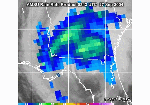
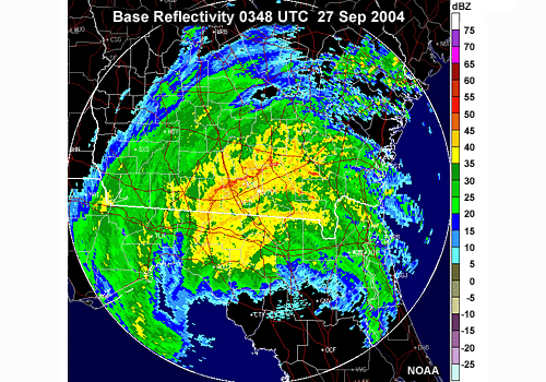
The NOAA Advanced Microwave Sounding Unit (AMSU) includes channels at 89 and 150 GHz that are well-suited for detecting frozen hydrometeors. We see a reasonable correlation between radar and satellite measurements in this comparison of the AMSU rain rate product and the radar base reflectivity.
The basis of the AMSU precipitation product is the scattering of microwaves by frozen precipitation. The equations used to determine the AMSU-derived precipitation allow for more accurate retrievals over land. This contrasts with the earlier SSM/I emission algorithms, which are more suitable for rainfall detection in marine environments.
Satellite Detection of Banded Precipitation » Discussion » Tropical Rainfall Measurement Mission (TRMM) Satellite Precipitation Radar

TRMM is the first satellite dedicated to measurement of rainfall over the global tropics. It travels an orbit which is inclined to the equator so that it covers an area between 35°N and 35°S. Each orbit takes about an hour and a half to complete. Consequently, all times of day and night are bp_d although any given locality may only be imaged once or twice a day.
The TRMM Precipitation Radar is the first satellite-based precipitation radar. It has a 4 km resolution, a 220 km swath width, and is able to detect rain rates as low as 0.7 mm/hr. In this comparison of the TRMM Precipitation Radar and radar base reflectivity, we see a strong correlation between the two images with detailed resolution in the satellite image. We can also see the narrow the 220-km satellite swath delineated by the red lines.
Satellite Detection of Banded Precipitation » Discussion » TRMM Microwave Imager (TMI)
The TRMM Microwave Imager, or TMI, measures the intensity of radiation at 10, 19, 22, 37, and 85 GHz. The four higher frequencies are similar to the SSM/I. The 10 GHz channel was designed to provide a more linear response for the high rainfall rates common in tropical rainfall. In this comparison, we can see how well the TMI rain rate product agreed with the composite radar reflectivity as Hurricane Jeanne came ashore in Florida.
By virtue of being in a lower orbit, the TMI provides better resolution than the SSM/I or the AMSU. However, this also results in a narrow swath across the surface. Unfortunately, the TMI is due to be terminated soon, but will eventually be replaced by even better instruments.
Satellite Detection of Banded Precipitation » Discussion » Blended Satellite-Derived Precipitation Products
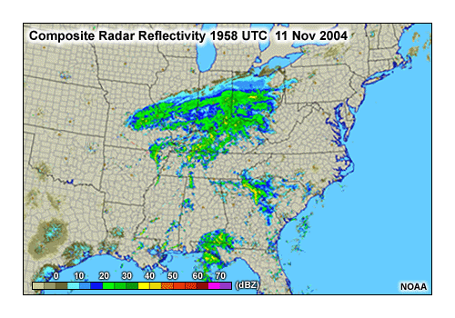
With all of these satellites presently in orbit, it was only a matter of time before all of the satellite-derived precipitation estimates were combined into one product. That time has come. The Naval Research Laboratory provides what we refer to as blended precipitation products, which are available online. Many other groups are also working on similar products. This image shows a 3 hour precipitation estimate derived from the NRL blended IR-microwave product. Compare that to the 3 hour composite radar plot for the same time period. Note the distinct similarity in both the location of precipitation as well as the local maxima.
With blended precipitation products, precipitation estimates derived from geostationary IR imagery are statistically tuned to agree with more accurate estimates from microwave sensors. The geostationary imagery is high frequency with vast areal coverage from 60°N to 60°S, but is not very accurate. In contrast, the microwave measurements are low frequency, but display high accuracy and high resolution. Microwave sensors include the TMI, SSM/I, and AMSU satellite instruments discussed previously.
The way blending works is that every 15° latitude/longitude box has its own calibration between IR temperature and precipitation. This calibration is continually updated based on the most recent microwave-derived precipitation estimates.
In addition to improved calibration, some of the other problems with IR-based precipitation estimates are also mitigated. Special tests are applied to detect and mitigate the effects of high cirrus clouds, to distinguish building versus dying storms, and to account for terrain enhancement.
While still not as accurate as surface-based radar, blended precipitation products provide a tremendous improvement in precipitation estimates in regions without radar coverage, including the world's oceans.
NRL Blended Rainrate Products are available at http://www.nrlmry.navy.mil/sat-bin/rain.cgi
Satellite Detection of Banded Precipitation » Discussion » Future Satellite Detection of Precipitation
A new generation of satellite sensors is due to be launched in the coming years. These include two of special interest for forecasting precipitation: the NPOESS CMIS and the GPM.
The National Polar Orbiting Earth Sensing Satellite Conical Microwave Imager Sounder, or NPOESS CMIS, builds on a number of passive microwave sensors from the last 25 years. CMIS represents a new era in storm monitoring, supplying data to forecasters in a matter of minutes after overpass, far faster than current polar-orbiting satellite systems. As shown here, CMIS will have a large, 2 meter antenna providing finer spatial resolution than previous microwave sensors. Like TMI, it will provide very high-resolution images, but with a wider 1700 km swath. Precipitation measurements will have an accuracy of 2 mm per hour.
The Global Precipitation Measurement or GPM is an international program that will operate a constellation of precipitation satellites. A series of satellites will carry radar and other microwave sensors to create global coverage of precipitation at 3 hour intervals. GPM technology is based on TRMM instrumentation. Although the GPM is primarily a research program, like the TRMM, it is anticipated that some GPM products will be useful for operational forecasting.
Further information on the GPM can be found at http://gpm.gsfc.nasa.gov. For more on the satellite detection of rainfall, see the COMET module Polar Satellite Products for the Operational Forecaster: Using Microwave Observations for Tropical Cyclone Analysis (https://www.meted.ucar.edu/npoess/tc_analysis/)
Satellite Detection of Banded Precipitation » Questions
Satellite Detection of Banded Precipitation » Questions » Question
Question 46
Which of the following satellites have a polar orbit? (Choose all that apply.)
The correct answers are b) and c).
GOES-8 is a geostationary satellite, which orbits the earth along the equatorial plane at the same speed as the earth's rotation. TRMM orbits along a plane that is inclined about 30 degrees to the equator. It's purpose is to measure tropical rainfall. SSM/I and AMSU travel a polar orbit and carry microwave imagers that detect precipitation.
Satellite Detection of Banded Precipitation » Questions » Question
Question 47
Which of the following satellites makes the most frequent observations of the Carribean? (Choose the best answer.)
The correct answer is a) GOES-10.
GOES-10 is a geostationary satellite positioned over the western Atlantic Ocean along the equator. It will typically image the Carribean at 3-hour intervals, and up to every 15 minutes in rapid-scan mode. TRMM will image the Carribean more frequently than SSM/I or AMSU because its orbit is only slightly inclined to the equator. SSM/I and AMSU typically capture images twice per day at low latitudes.
Satellite Detection of Banded Precipitation » Questions » Question
Question 48
Which of the following microwave imagers has the highest resolution and the narrowest swath? (Choose the best answer.)
The correct answer is c) TMI.
The TRMM Microwave Imager (TMI) has the lowest orbit. This results in the highest resolution and the narrowest swath among the current generation of microwave imagers.
Satellite Detection of Banded Precipitation » Questions » Question
Question 49
What are some of the advantages of a blended precipitation product? (Choose all that apply.)
The correct answers are a) and c).
Blended precipitation products frequently recalibrate the IR temperature to precipitation rate using the latest estimate available from microwave imagers. Because the product relies on GOES IR imagery, it has a relatively high frequency, typically every 3 hours. One limitation is that imagery from geostationary satellites is limited to the area from 60°N to 60°S. High-latitude regions are not covered.
Summary
Precipitation bands are simply linear regions of enhanced rain or snow. These bands are typically diagnosed in real time with radar or satellite imagery, but may also be identified in the forecast precipitation fields from numerical model output.
Precipitation bands often occur in conjunction with extratropical cyclones, especially near frontal zones. These systems are often accompanied by a trowal airstream, a flow of relatively warm, moist air ascending along the sloping intersection of the aging warm and cold fronts, roughly parallel to the surface occluded front.
The occurrence of precipitation requires sufficient moisture and lift. Convection requires the additional ingredient of instability. Of the tools that we examined in this module, perhaps the most useful is frontogenesis. It is especially useful because it is comprised of deformation as well as convergence; both may lead to linear regions that may support precipitation. Melting-induced circulations, frontal merger, and conditional symmetric instability frequently occur near regions of significant frontogenesis. Clearly, frontogenesis products are a valuable means by which we can search for potential banding events in background fields of moisture and ascent.
Many precipitation bands are convective in nature. Unfortunately, many numerical weather models do not handle this process well. Large grid spacings and hydrostatic architecture can prevent models from accurately representing rain and snowbands resulting from convection. However, such models are not completely incapable of predicting the development of banded precipitation. Even if the precipitation field is not entirely accurate, the larger dynamic fields such as temperature, heights, wind, and vertical motion are usually handled well.
In short, a model precipitation forecast may be useful, but it is not foolproof. Users of numerical model output should always examine more basic vertical motion and moisture fields, and assess how they compare to the model precipitation fields. Ideally, they will be in close agreement. If not, forecasters should view their model solutions closely and with some suspicion when trying to forecast banded precipitation events.
References
Bibliography
Air Weather Service Manual, 1979: Use of the skew-T, log P diagram in analysis and forecasting. AWS-TM 79-006, Department of the Air Force, 95 pp. [Available from Department of the Air Force, USAF, ETAC, Scott Air Force Base, IL 62225-5458]
Browning, K. A., 1988: Chapter in Palmn Memorial Symposium on Extratropical Cyclones: Helsinki, Finland, 29 Aug.-2 Sept. 1988, Geophysical Society of Finland, American Meteorological Society.
Browning, K. A., 1990: Organization and internal structure of synoptic and mesoscale precipitation systems in midlatitudes. Radar in Meteorology, David Atlas, Ed., Battan Memorial and 40th Anniversary Radar Meteorology Conference, American Meteorological Society, pp. 433-460.
Browning, K. A., 1990: Rain, rainclouds and climate. Quart. J. Roy. Meteor. Soc., 116, 1025-1051.
Browning, K. A., and G. A. Monk, 1982: Simple model for the synoptic analysis of cloud fronts. Quart. J. Roy. Meteor. Soc., 108, 435-452.
Carlson, T. N., 1980: Airflow Through Midlatitude Cyclones and the Comma Cloud Pattern. Mon. Wea. Rev., 108, 14981509.
Carr, F. H., and Millard, J. P., 1985: A Composite Study of Comma Clouds and their Association with Severe Weather over the Great Plains. Mon. Wea. Rev., 113, 370387.
Coleman, H., and Marwitz, J., 2002: Thermodynamic and Kinematic Structure of a Snowband and Freezing Rain Event during STORM-FEST. Wea. Forecasting, 17, 2746.
Dunn, L. B., cited 2004: CSI Snow Event Over Wasatch Front. Western Region Technical Attachment 99-05. Available online at [www.wrh.noaa.gov/slc/projects/csi_990304/csi_990304.html]
Glass, F. H., D. L. Ferry, J. T. Moore, and S. M. Nolan, 1995: Characteristics of heavy convective rainfall events across the mid-Mississippi valley during the warm season: Meteorological conditions and a conceptual model. Preprints, 14th Conf. on Weather Forecasting and Analysis, Dallas, Texas, American Meteorological Society, 3441.
Graves, C. E., J. T. Moore, M. J. Singer, and S. Ng, 2003: Band on the Run - Chasing the Physical Processes Associated with Heavy Snowfall. Bull. Amer. Meteor. Soc., 84, 990994.
Johns, R. H., and C. A. Doswell, III, 1992: Severe local storms forecasting. Wea. Forecasting, 7, 588-612.
Market, P. S., and D. Cissell, 2002: Formation of a Sharp Snow Gradient in a Midwestern Heavy Snow Event. Wea. Forecasting, 17, 723738.
Market, P. S., and J. T. Moore, 1998: Mesoscale Evolution of a Continental Occluded Cyclone. Mon. Wea. Rev., 126, 17931811.
Martin, J. E., 1998: The Structure and Evolution of a Continental Winter Cyclone. Part I: Frontal Structure and the Occlusion Process. Mon. Wea. Rev., 126, 303328.
Martin, J. E., 1998: On the Deformation Term in the Quasigeostrophic Omega Equation. Mon. Wea. Rev., 126, 20002007.
Martin, J. E., 1999: Quasigeostrophic Forcing of Ascent in the Occluded Sector of Cyclones and the Trowal Airstream. Mon. Wea. Rev., 127, 7088.
McDonnal, D., and B. Colman, cited 2004: An Investigation of the Puget Sound Convergence Zone Using WES. Available online at [www.wrh.noaa.gov/wrhq/talite44.htm]
Moore, J. T., and K. F. Smith,, 1989: Diagnosis of Anafronts and Katafronts. Wea. Forecasting, 4, 6172.
Neiman, P. J., F. M. Ralph, M. A. Shapiro, B. F. Smull, and D. Johnson, 1998: An Observational Study of Fronts and Frontal Mergers over the Continental United States. Mon. Wea. Rev., 126, 25212554.
Nicosia, D. J., and R. H. Grumm, 1999: Mesoscale Band Formation in Three Major Northeastern United States Snowstorms. Wea. Forecasting, 14, 346368.
Ninomiya, K., 1971: Mesoscale Modification of Synoptic Situations from Thunderstorm Development as Revealed by ATS III and Aerological Data. J. Appl. Meteor., 10, 11031121.
Novak, D. R., L. F. Bosart, D. Keyser, and J. S. Waldstreicher, 2002, cited 2004: A climatological and composite study of cold season banded precipitation in the northeast United States. Preprint, 19th Conference on Weather Analysis and Forecasting. San Antonio, TX, American Meteorological Society. Available online at [http://cstar.cestm.albany.edu/preprints/novakWAF.pdf]
Rose, S. F., P. V. Hobbs, J. D. Locatelli, and M. T. Stoelinga, 2002: Use of a Mesoscale Model to Forecast Severe Weather Associated with a Cold Front Aloft. Wea. Forecasting, 17, 755-773.
Samson, H. W., 1951: A study of cold fronts over the British Isles. Quart. J. Roy. Meteor. Soc., 77, 96-120.
Shapiro, M. A., and D. Keyser, 1990: Fronts, jet streams, and the tropopause. Boulder, Colorado, U.S. Department of Commerce, National Oceanic and Atmospheric Administration, Environmental Research Laboratories, 1990. 75 pp.
Steigerwald, H., 1986: Deformation zones and heavy precipitation. Natl. Wea. Dig., 11, 1520.
Szeto, K. K., and R. E. Stewart, 1997: Effects of Melting on Frontogenesis. J. Atmos.Sci., 54, 689702.
Relevant COMET Modules
Diagnosing and Forecasting Extratropical Transition: A Case Exercise on Hurricane Michael (https://www.meted.ucar.edu/norlat/ett/michael/)
How Mesoscale Models Work (https://www.meted.ucar.edu/mesoprim/models/)
Hurricanes Canadian Style: Extratropical Transition (https://www.meted.ucar.edu/norlat/ett/)
Operational Models Matrix (https://sites.google.com/ucar.edu/operational-models-encyclo/home)
Polar Lows, Ungava Bay 01 December 2000 (https://www.meted.ucar.edu/norlat/snow/polarlow_case/)
Polar Satellite Products for the Operational Forecaster: Using Microwave Observations for Tropical Cyclone Analysis (https://www.meted.ucar.edu/npoess/tc_analysis/)
Principles of Convection III: Shear and Convective Storms (https://www.meted.ucar.edu/mesoprim/shear/)
Quantitative Precipitation Forecasting Overview (https://www.meted.ucar.edu/qpf/qpfintro/)
Severe Convection II: Mesoscale Convective Systems (https://www.meted.ucar.edu/mesoprim/severe2/)
Slantwise Convection: An Operational Approach (https://www.meted.ucar.edu/norlat/slant/)
Topics in Polar Low Forecasting (https://www.meted.ucar.edu/norlat/snow/polarlows/)
Contributors
The following have contributed to the development of Mesoscale Banded Precipitation
Sponsors
- National Oceanic and Atmospheric Administration (NOAA)
- National Weather Service (NWS)
- Naval Meteorology and Oceanography Command (NMOC)
- Air Force Weather Agency (AFWA)
- National Environmental Satellite Data and Information Service (NESDIS)
- National Polar-orbiting Operational Environmental Satellite System (NPOESS)
- Meteorological Service of Canada (MSC)
Project Contributors
Principal Science Advisor
- Dr. Patrick S. Market - University of Missouri - Columbia
Additional Science Advisors
- CDR Berdequez - Naval Meteorology and Oceanography Professional Development Center (NAVMETOCPRODEVCEN)
- Staff at HQ AFWA/DNT 28th OWS Training Flight - Shaw AFB
- Thomas Lee - Naval Research Laboratory - Monterey
- Dr. Wendell Nuss - Naval Postgraduate School
Project Co-lead/Instructional Design/Multimedia Authoring
- Dr. Alan Bol - UCAR/COMET
Project Co-lead/Project Meteorologist
- Dr. Doug Wesley - UCAR/COMET
Project Meteorologist
- Dr. Arlene Lainge - UCAR/COMET
Illustration/Multimedia Authoring
- Steve Deyo - UCAR/COMET
Graphic Interface Design/Illustration/Multimedia Authoring
- Heidi Godsil - UCAR/COMET
Audio Editing/Production/Multimedia Authoring
- Seth Lamos - UCAR/COMET
Multimedia Authoring
- Carl Whitehurst - UCAR/COMET
Audio Narration
- Steven Saint James
- Wendy Abshire - UCAR/COMET
Software Testing/Editing/Quality Assurance
- Linda Korsgaard - UCAR/COMET
- Michael Smith - UCAR/COMET
Copyright Administration
- Lorrie Alberta - UCAR/COMET
Images and Photographs Provided by
- Naval Research Laboratory - Monterey
- NOAA
- U.S. Air Force
COMET HTML Integration Team 2021
- Tim Alberta — Project Manager
- Dolores Kiessling — Project Lead
- Steve Deyo — Graphic Artist
- Ariana Kiessling — Web Developer
- Gary Pacheco — Lead Web Developer
- David Russi — Translations
- Tyler Winstead — Web Developer
COMET Staff, June 2005
Director
- Dr. Timothy Spangler
Deputy Director
- Dr. Joe Lamos
Meteorologist Resources Group Head
- Dr. Greg Byrd
Business Manager / Supervisor of Administration
- Elizabeth Lessard
Administration
- Lorrie Alberta
- Heather Hollingworth
- Linda Korsgaard
- Bonnie Slagel
Graphics / Media Production
- Steve Deyo
- Heidi Godsil
- Seth Lamos
- Dan Riter
Hardware / Software Support and Programming
- Tim Alberta (Supervisor)
- James Hamm
- Karl Hanzel
- Ken Kim
- Mark Mulholland
- Carl Whitehurst
Instructional Design
- Patrick Parrish (Supervisor)
- Dr. Alan Bol
- Lon Goldstein
- Dr. Vickie Johnson
- Bruce Muller
- Katherine Olson
- Dwight Owens
- Dr. Sherwood Wang
Meteorologists
- Dr. William Bua
- Patrick Dills
- Tom DuLong
- Kevin Fuell
- Patrick Hofmann (Student Assistant)
- Dr. Stephen Jascourt
- Matthew Kelsch
- Dolores Kiessling
- Dr. Arlene Laing
- Elizabeth Page
- Wendy Schreiber-Abshire
- Dr. Doug Wesley
Software Testing / Quality Assurance
- Michael Smith (Coordinator)
National Weather Service COMET Branch
- Dr. Rick Koehler
- Anthony Mostek (National Satellite Training Coordinator)
- Brian Motta
- Dr. Robert Rozumalski (SOO/SAC Coordinator)
Meteorological Service of Canada Visiting Meteorologists
- Peter Lewis
- Garry Toth