Produced by The COMET® Program
Welcome
Welcome to Distributed Hydrologic Models for Flow Forecasts. My name is Dennis Johnson and I'm a professor at Juniata College in Pennsylvania.
Objectives
The primary goal of Part 1 of this two-module series is to describe distributed hydrologic models and how they work. We'll look at understanding the differences between lumped and distributed models, how lumped models may be subdivided for example into grids, sub-basins, or flow planes, and when distributed hydrologic models are most appropriate. We'll talk about distributed models and how they tend to rely on physically-based approaches, while lumped models rely on conceptual approaches. Finally, we'll look at some of the challenges of applying distributed hydrologic models.
Hydrologic Model
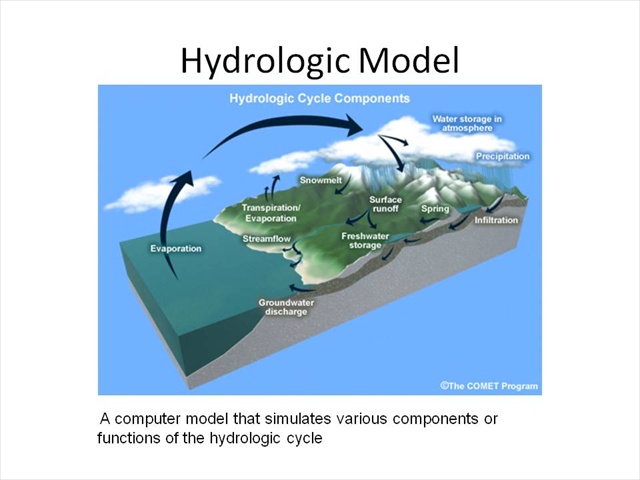
For the purposes of this module, we will consider the term hydrologic model to be a computer model that simulates various components or functions of the hydrologic cycle.
The simulation capabilities vary in terms of both space and time – some models look at long time steps or scales , while others may use short time steps and simulate a relatively short time span – as in the case of a flash flood.
Output

Before we move forward, let's consider some of the more basic and common functions of a hydrologic model.
The output of hydrologic models varies – depending on the goals and objectives of the model. Some models are used to predict monthly runoff totals, while others are designed to look at individual storm events.
Perhaps the most common output is the hydrograph or runoff hydrograph.
For more information refer to the Basic Hydrologic Sciences Distance Learning Course.
Question
Hydrologic models, whether lumped or distributed, have a common goal of determining the fate of the precipitation at the end of each time step.
The correct answer is a) True
Both modeling approaches compute a variety of functions to simulate the fate of the precipitation at distinct time steps. The difference is that distributed models must do these tasks on all of the sub-elements of a watershed, as we shall observe through the course of this module.
Characteristics
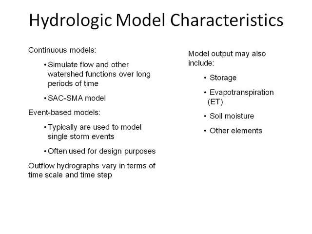
Some models may be developed as continuous models – these are used to simulate flow and other watershed functions (e.g., storage) over long periods of time. The SAC-SMA model is often used in this fashion.
Other models are more event-based models and typically are used to model single storm events. These models are often used for design purposes (e.g. designing a culvert to pass the 100–year event).
Thus, the model outflow hydrographs could vary greatly in terms of time scale and time step.
Besides runoff hydrographs, models may also output information as storage, evapotranspiration, soil moisture, and other elements – this of course depends on the aforementioned goals and objectives of the model itself.
For more information refer to the Basic Hydrologic Sciences Distance Learning Course.
Functions
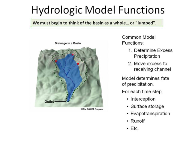
Let's start with the basic goal of a hydrologic model – the rainfall runoff process itself. We must begin to think of the basin as a whole – a single entity. The precipitation (usually a time series) is generally passed to the model.
Once the rain has been "passed" to the model, the model must now determine the fate of the precipitation – generally in distinct time steps. So for each time step, we hear words like interception, surface storage, evapotranspiration, and runoff to name but a few. These are all examples of common watershed functions that are simulated within the watershed model.
Thus, the model outflow hydrographs could vary greatly in terms of time scale and time step.
In a general sense, 2 of the more common functions within a time step are : 1) determining the excess precipitation and 2) moving the excess precipitation off the land surface to the receiving stream or channel.
"Fate of Precipitation"
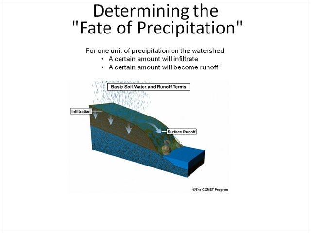
At the most basic level, we may say something like this: "if 1 unit of precipitation falls on the watershed, then a certain amount will infiltrate and a certain amount will become runoff". This is the fate of the precipitation. Most hydrologic models have a function to do just that – determine the fate. Some are relatively simple such as the NRCS Runoff Curve Number, while others are more complex, in which an accounting system is used to keep continuous track of the watershed properties. Regardless, let's keep this basic model in mind and realize that at the end of each time step, a certain depth of excess precipitation may be available for runoff.
Unit Hydrograph
Unit Hydrograph Approach 1
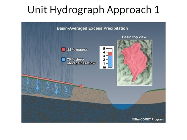
The second common function of the model is to "move" or "route" the excess precipitation off of the watershed and onto the receiving stream. One of the most common methods for doing this is the unit hydrograph approach. It is assumed that the student is familiar with unit hydrograph concepts. There is also a distance learning module available on Unit Hydrograph Theory at COMET.
Unit Hydrograph Approach 2
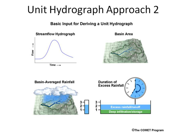
Basically, the unit hydrograph transforms the excess precipitation from a uniform depth distributed over an area to an outflow hydrograph.
The timing and shape of the hydrograph are a function of various watershed parameters such as area, slope, and lengths. There are other methods to move the water to the outlet, such as a kinematic wave overland flow method. In this method, the excess is routed downslope to the outlet or receiving stream using the kinematic wave routing technique.
See Unit Hydrograph Theory module for more information.
Streamflow Components
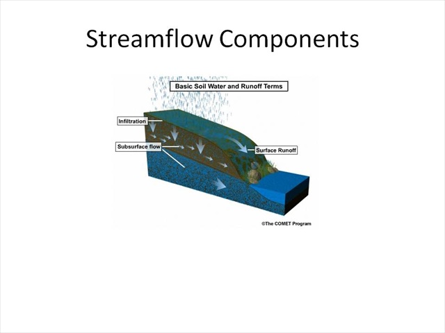
One important note is that excess precipitation may not be just surface excess. In hydrologic models, streamflow can be generated from overland or surface flow or flow that is in the subsurface.
The SAC-SMA Model
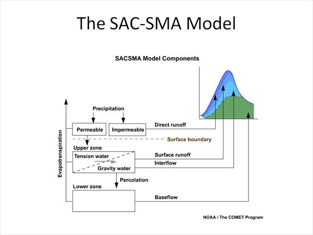
What you're looking at here is the SAC-SMA. After each time step, water is available for streamflow from a variety of components, whether they be surface, upper zone, or lower zone.
Moving Excess Precipitation
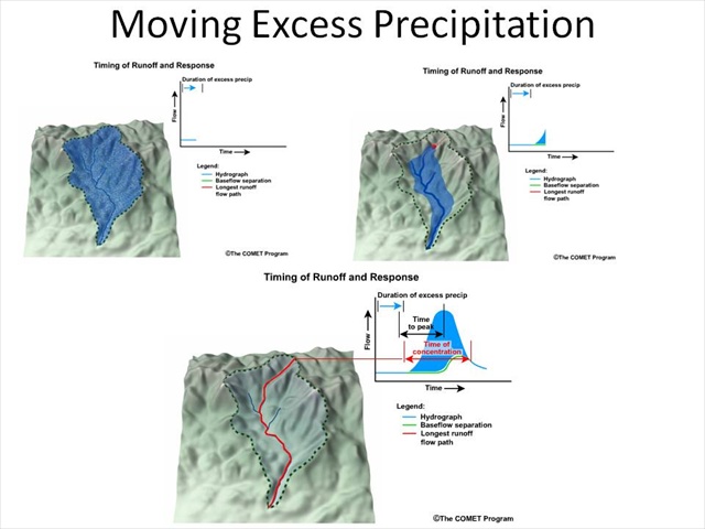
So in each time step, we have the rainfall coming in, the model determines the excess and then moves the excess to the outlet to create the hydrograph.
The Lumped Model
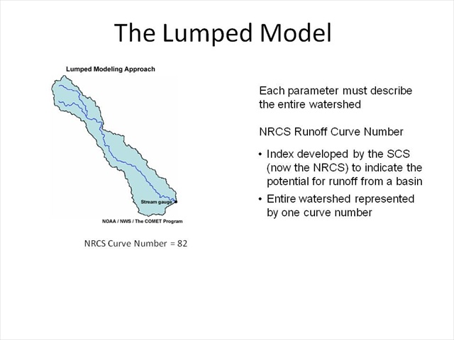
Quite often, this is all done in a lumped model – a model where each parameter that describes the watershed must describe the entire watershed. We think of the watershed as a whole. Take, for example, the NRCS Runoff Curve Number. The Curve Number is an index developed by the SCS (now the NRCS) to indicate the potential for runoff from a basin.
In using the NRCS Runoff Curve Number in a lumped model, the entire watershed is represented by one curve number – although it may be a weighted value – it is still one value with no regard for spatial variation.
Question
Question 1 of 2
A basin contains primarily dry soil in the upper two-thirds of the watershed and wet soil in the lowest third. In a lumped model, how many values will be used to parameterize soil conditions for this basin?
The correct answer is b) 1
A lumped model will use one value to parameterize soil conditions for the basin.
Question 2 of 2
In a lumped model, what value would be used to parameterize the soil conditions for a watershed with dry soil in the upper two-thirds and wet soil in the lowest third?
The correct answer is c) A weighted average of the wet soil and dry soil values (2/3 Xdry + 1/3 Xwet)
The soil conditions will be parameterized by a weighted average. Spatial variations in land use or land cover can be accounted for using a weighted average for the basin. This weighted average represents the basin as a whole but cannot illustrate the exact spatial locations of the various parameters that were used to determine the final value.
SAC-SMA Application
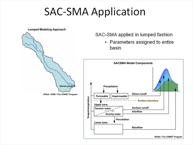
In a more complex situation, the SAC-SMA can be applied in a lumped fashion. In this case, the entire basin or sub-basin is assigned a set of parameters. These parameters represent how the basin acts or behaves as a whole—not necessarily a representation of a single point. Even beyond computing excess precipitation, the unit hydrograph operation works in a similar fashion: the entire watershed is assumed to be represented by the shape of the unit hydrograph.
Average Over Watershed
Average Over Watershed 1
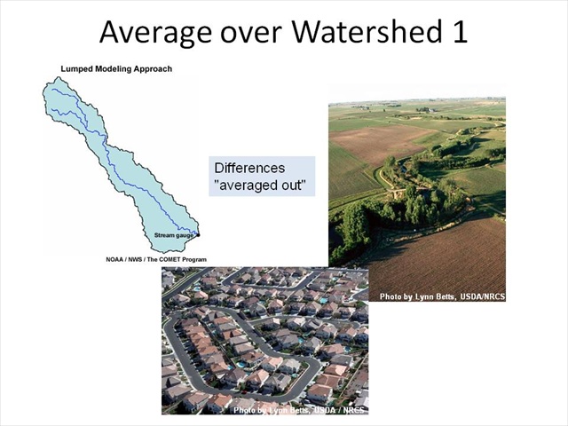
When we lump, we are essentially coming up with a value (hopefully through calibration) that represents how the entire watershed behaves. We intuitively know that the entire watershed cannot all be represented by a single value. We realize that changes in land use or soil depth will obviously change responses; however, in a lumped model we basically average out these differences. You're going to hear this term "average out" quite often. Even if a watershed is all one type of land use – such as agriculture or urban, there may be considerable variations within the watershed that create spatial differences.
Average Over Watershed 2
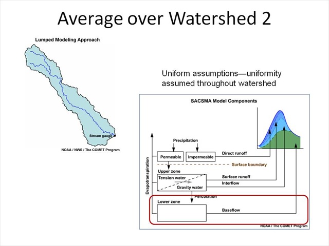
We often talk about uniform assumptions. The parameters used to describe the watershed assume uniformity throughout the watershed. Using the SAC-SMA model, we would, for example, assume that the lower zone free water is uniform throughout the entire watershed.
Lumped Model Weaknesses
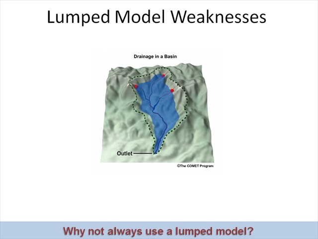
If our only goal is to simulate runoff at the outlet of a watershed, then lumped models have been time tested and perform quite well.
So you might ask, why not always use a lumped model? We're going to spend a few minutes looking at some scenarios where lumped models may not work well, and we need to move to a distributed model.
Storm Area Small for Watershed
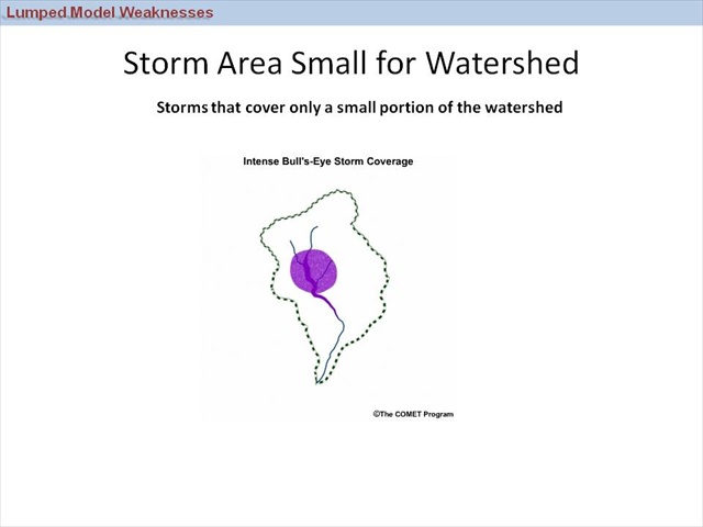
In this first scenario, we have a storm that is relatively small compared to the watershed itself. In this case, the rainfall is hitting only a small portion of the watershed and the mean areal precipitation (MAP) will not accurately represent the distribution of the precipitation. Local areas that have high intensities and can generate runoff – even flooding -- are not properly simulated. The well-calibrated lumped model may show little or no runoff due to the MAP being the average over the entire basin.
Question
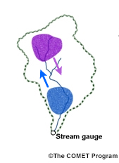
How would you expect the flow at stream outlet to differ for a downstream-moving storm versus a upstream-moving storm?
The correct answer is a)
Storm Direction
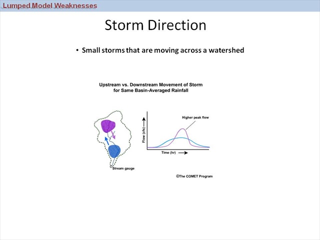
Similar to the first scenario, small storms that are moving, either up or down the watershed or even across the watershed, tend to pose difficulties for the lumped models. In this case, the mean aerial precipitation is not the only issue, but the direction of the storm movement can also cause problems.
Storm Coverage
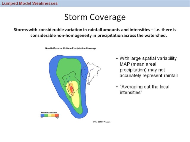
All storms have some level of variability. There may be times however, when storms have a large amount of variability in either space or time. In the case of spatial variability, the mean areal precipitation (MAP) may not accurately represent the actual rainfall that fell over the basin because there is an averaging, or smoothing, out. Sometimes we talk about this as averaging out the local intensities.
Watershed State
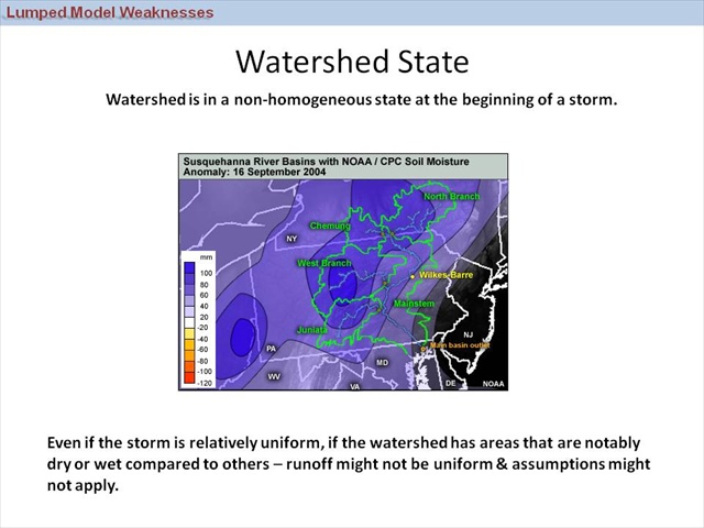
Similarly to variability in the rainfall, there may also be times when the watershed itself is in a very non-homogeneous state. For example, soil moisture may vary throughout the watershed. This can be caused by variations in land use or land cover, soil properties, physical characteristics such as slope and aspect, or even antecedent rainfall. When we subdivide into smaller watersheds or smaller elements, the soil moisture distribution hopefully becomes more uniform.
Additional Locations
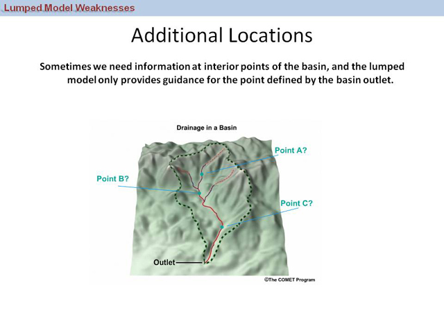
This last case is simply a need for more data. Sometimes, we just want more information within the watershed itself, not just at the outlet.
Summary: Weaknesses of Lumped Models
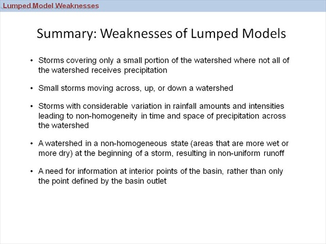
The points we see here are examples of times when lumped models may not perform well – there are certainly others and there are variations of those listed.
In order to address any of these situations, we simply need more information within the watershed. We need to have more information at a finer or more detailed scale. In short, we need to distribute the descriptive parameters throughout the watershed as opposed to a single lumped value.
Subdividing the Basin
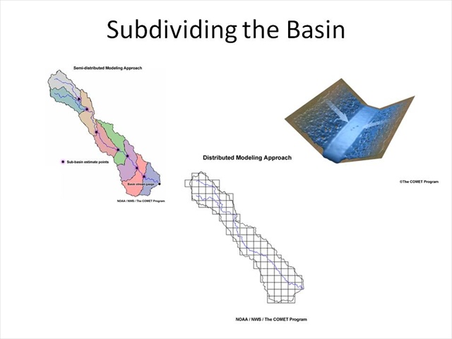
Once we have determined that some type of a distributed model may be more appropriate, we must now consider the manner in which we will break down the watershed. We do this by breaking the model into smaller sub-sections.
Sub-basins
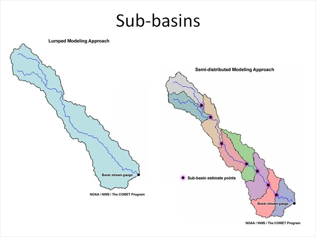
The most basic and perhaps most common approach would be to subdivide the watershed into smaller watersheds or sub-basins. These are intended to be more homogeneous in nature. By subdividing the watershed, we can hopefully avoid many of the deficiencies in lumped models—some of which were previously discussed.
Planes
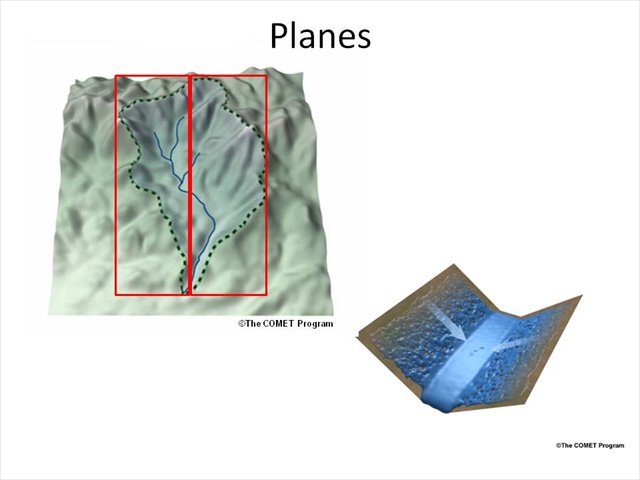
Besides subdividing the watershed into smaller watersheds or sub-basins, some models break the watershed into other elements. For example, flow planes have been used by some modelers. All are considered to be homogeneous in nature and sloped towards the stream.
Moving Water Over a Plane
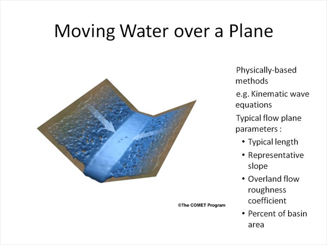
As a side note, when a watershed is discretized into some number of distinct flow planes, it is quite common to use more physically-based methods to move the excess precipitation off of the watershed. An example of this is the kinematic wave equations. We won't go into detail of this method, but the parameters that are commonly required include lengths, slopes, a roughness coefficient, and sometimes the percent of the basin that is covered by each plane.
Grids
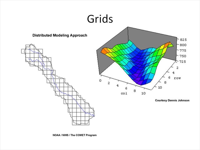
While there are multiple ways to subdivide a watershed, one of the more common methods – as of late – has been to break the watershed into grids. We have probably all seen a gridded representation of the earth's surface in one form or another.
This has been greatly enhanced through GIS data sets and in particular fairly high resolution digital elevation models or DEMs, as well as other data sets and satellite data.
The Juniata River Watershed
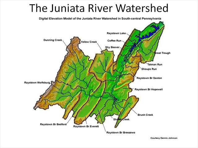
Here we see a digital elevation model of the Juniata River Watershed in south-central Pennsylvania. The sub-watersheds are also noted, as are the major streams and rivers.
Gridded Representation
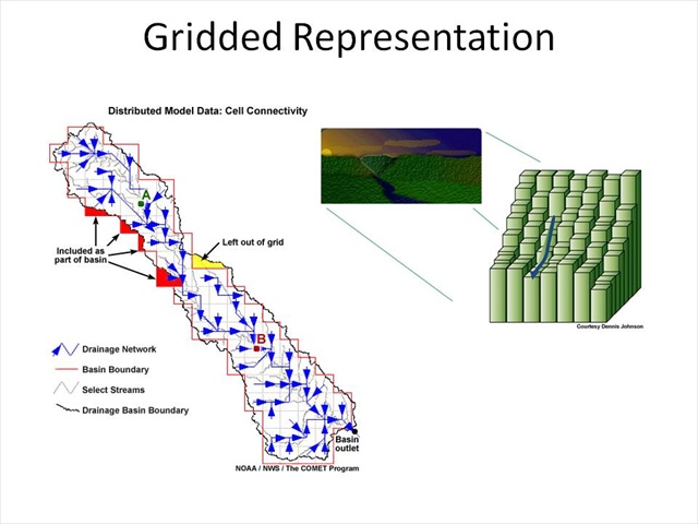
Basically, we can think of the earth's surface as being represented by a series of 3-dimensional blocks with flow (both on the surface and subsurface) flowing from one block to another. Most commonly, this is done by having the flow go to the neighboring block with the greatest downslope gradient.
Question
Would you expect a distributed model to require “lumping” or averaging of descriptive parameters?
The correct answer is c)
In a distributed model, there is still some degree of averaging or lumping. Consider a hydrologic model that uses a 10m Digital Elevation Model to describe the watershed. There would still be averaging over the 10m x 10m grid cells. The difference is that the degree of spatial variability over a small grid cell is small compared to variability for a 30 km2 watershed.
Many More Parameters!
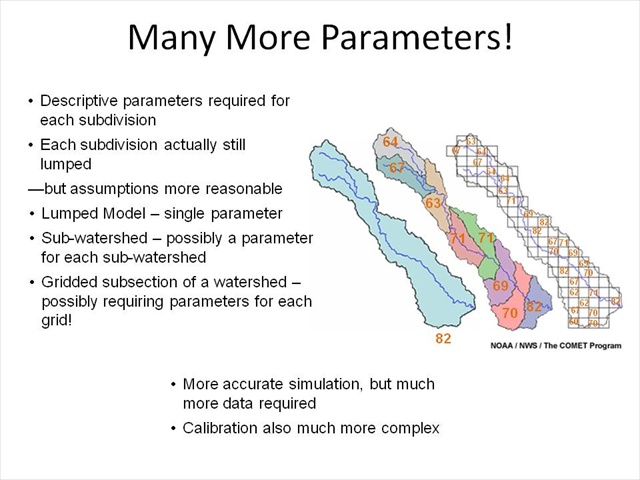
Regardless of the manner of subdivision, the modeler must now provide descriptive parameters, not for the watershed, but for each of the subdivided elements! We have thus distributed the parameters across the watershed. In truth, there is still lumping as each subdivision is now considered to be homogeneous in itself. But the area over which the parameter is applied hopefully now sufficiently small enough that we are more comfortable with the assumption of uniformity over the element.
For example, consider the NRCS curve number method again, in a lumped watershed, there would be one curve number. In a distributed watershed, there could be a curve number for every subdivision – be it grids, planes, or just sub-watersheds. The SAC-SMA would be even more complex. In a lumped model, there is one set of SAC parameters, in a distributed model, you could have a different set of SAC parameters for each subdivision!
So now, we have the watershed subdivided and will hopefully be able to provide a more accurate simulation of watershed response; however, we now must provide considerably more data. In addition, the concept of calibrating a distributed model is much more complex – as we now have multiple (possibly thousands or more) individual elements to calibrate. This will be discussed at a later point.
Distributed Models Build on Lumped
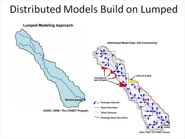
Recall for a moment the lumped model. The lumped model is basically one element and for each time step the model determines the fate of the rainfall and then moves the excess to the watershed outlet.
Let's consider a gridded model. This concept is basically the same. It is just done on each element or grid instead of one lumped element.
For each time step, the model determines the fate of the precipitation (which must be distributed to match the watershed subdivisions). Excess precipitation is then "moved" to the outlet in some fashion. Again, the excess could come from either the surface or from elements in the subsurface (e.g. lower zone free water in the Sacramento model or SAC-SMA).
Subsurface Flow Limitations
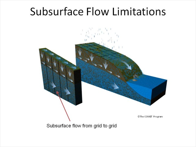
One of the more difficult aspects of grid-based modeling is the movement of subsurface flow. Subsurface flow patterns vary greatly and are much more difficult to model or even measure in the field on a grid to grid basis. This is sometimes viewed as an inherent weakness in some distributed models.
Because of this, many distributed models perform better on runoff events that tend to be dominated by surface runoff, which is often called direct runoff. Small intense storms or flash flood events are prime examples of this.
Physically-based Approach
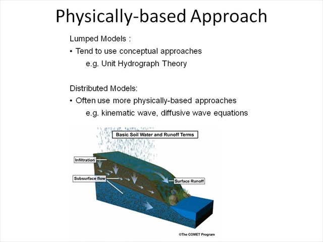
In the lumped models, we tended to use more conceptual approaches (e.g. Unit Hydrograph Theory), while in a distributed model, we often resort to more physically based approaches, such as the kinematic wave or even diffusive wave equations. Although, there are certainly exceptions to this and even combinations of model types, we still tend to see more physically-based approaches in distributed models.
Physically-based Model Advantages
In some instances, the use of physically-based approaches may provide an advantage over conceptual approaches in a distributed hydrologic model as physically-based models attempt to simulate processes based on the governing physical equations. These equations, in turn, often rely on physical characteristics of the watershed (e.g. slope, lengths, areas, and soil characteristics). These data are often more available than data used to populate some conceptual models.
As a result, physically based models may also perform better in areas where measurements and observations are sparse.
DHM Key Points
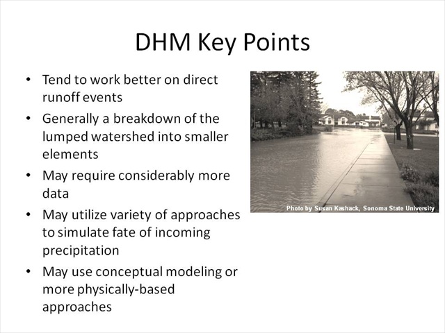
DHMs tend to work better on events that are direct runoff dominated, such as flood floods.
A distributed model is generally a breakdown of the lumped watershed into smaller elements and the distribution of parameters may require considerably more data.
The distributed modeling system can utilize a number of different approaches, just like a lumped model, to simulate the fate of the incoming precipitation.
Some may use conceptual modeling approaches (SAC-SMA) and others may use a more physically-based approach.
This concludes Part I of Distributed Hydrologic Models for Flow Forecasts. In Part II we will look further into distributed models and consider issues such as calibration and data assimilation. We will also discuss approaches for selecting a model for various flow forecasting situations.
Next Steps
Congratulations!
You have completed Distributed Hydrological Models for Flow Forecasts Part 1 of 2.
Please remember to complete the quiz for this module. We would also like to invite you to take a moment to provide us with your comments and feedback by completing a brief user survey. The quiz and survey may be accessed from the menu at the top of this module.
For more additional information on climate and weather-related topics go to:
www.meted.ucar.edu
Note to NOAA/NWS users:
If you accessed this module through the NWS Learning Center, you must return to that system to complete the quiz in order to receive credit for completion.
Contributors
COMET Sponsors
The COMET® Program is sponsored by NOAA National Weather Service (NWS), with additional funding by:
- Air Force Weather (AFW)
- Australian Bureau of Meteorology (BoM)
- European Organisation for the Exploitation of Meteorological Satellites (EUMETSAT)
- Meteorological Service of Canada (MSC)
- National Environmental Education Foundation (NEEF)
- National Polar-orbiting Operational Environmental Satellite System (NPOESS)
- NOAA National Environmental Satellite, Data and Information Service (NESDIS)
- Naval Meteorology and Oceanography Command (NMOC)
Project Contributors
Principal Science Advisor
- Dr. Dennis Johnson — Juniata College
Additional Science Advisors
- Matt Kelsch — UCAR/COMET
- Dr. Pedro Restrepo — NOAA/NWS
- Mike Smith — NOAA/NWS
Project Lead (Science)
- Amy Stevermer — UCAR/COMET
Project Lead (Instructional Design)
- Lon Goldstein — UCAR/COMET
Graphics/Interface Design
- Steve Deyo — UCAR/COMET
- Brannan McGill — UCAR/COMET
Multimedia Authoring
- Lon Goldstein — UCAR/COMET
Audio Editing/Production
- Seth Lamos — UCAR/COMET
Audio Narration
- Dr. Dennis Johnson — Juniata College
COMET HTML Integration Team 2020
- Tim Alberta — Project Manager
- Dolores Kiessling — Project Lead
- Steve Deyo — Graphic Artist
- Gary Pacheco — Lead Web Developer
- Justin Richling — Associate Scientist
- David Russi — Translations
- Gretchen Throop Williams — Web Developer
- Tyler Winstead — Web Developer
COMET Staff, July 2009
Director
- Dr. Timothy Spangler
Deputy Director
- Dr. Joe Lamos
Administration
- Elizabeth Lessard, Administration and Business Manager
- Lorrie Alberta
- Michelle Harrison
- Hildy Kane
Hardware/Software Support and Programming
- Tim Alberta, Group Manager
- Bob Bubon
- James Hamm
- Ken Kim
- Mark Mulholland
- Wade Pentz, Student
- Jay Shollenberger, Student
- Malte Winkler
Instructional Designers
- Dr. Patrick Parrish, Senior Project Manager
- Dr. Alan Bol
- Lon Goldstein
- Bryan Guarente
- Dr. Vickie Johnson
- Tsvetomir Ross-Lazarov
- Marianne Weingroff
Media Production Group
- Bruce Muller, Group Manager
- Steve Deyo
- Seth Lamos
- Brannan McGill
- Dan Riter
- Carl Whitehurst
Meteorologists/Scientists
- Dr. Greg Byrd, Senior Project Manager
- Wendy Schreiber-Abshire, Senior Project Manager
- Dr. William Bua
- Patrick Dills
- Dr. Stephen Jascourt
- Matthew Kelsch
- Dolores Kiessling
- Dr. Arlene Laing
- Dr. Elizabeth Mulvihill Page
- Amy Stevermer
- Warren Rodie
- Dr. Doug Wesley
Science Writer
- Jennifer Frazer
Spanish Translations
- David Russi
NOAA/National Weather Service - Forecast Decision Training Branch
- Anthony Mostek, Branch Chief
- Dr. Richard Koehler, Hydrology Training Lead
- Brian Motta, IFPS Training
- Dr. Robert Rozumalski, SOO Science and Training Resource (SOO/STRC) Coordinator
- Ross Van Til, Meteorologist
- Shannon White, AWIPS Training
Meteorological Service of Canada Visiting Meteorologists
- Phil Chadwick
- Jim Murtha