Introduction
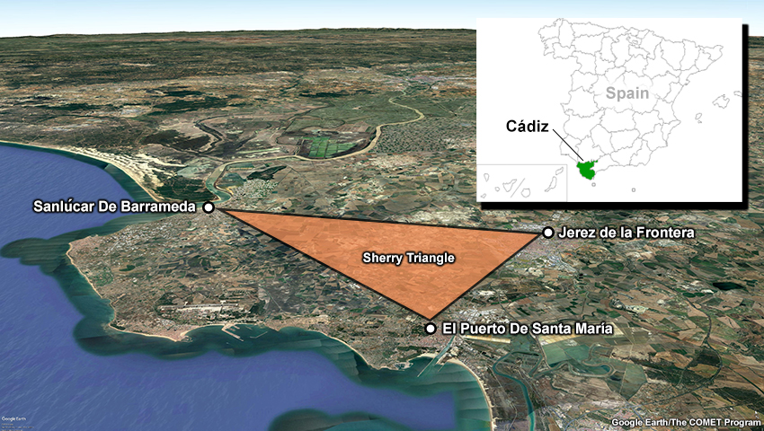
The Sherry Triangle, an area in the province of Cádiz in southwestern Spain that is known for its sherry wine production.
Spain is one of the world’s largest wine producers; grapes are an important commodity of the country’s agriculture industry.
Imagine you are a solar engineer consulting with a farmer about their vineyard in the Sherry Triangle, an area in southwestern Spain known for its sherry wine production. Due to the increased demand for sherry, farmers growing white grapes in the city of Jerez de la Frontera are interested in installing solar electric panels to help reduce electric costs for powering farm operations. You were sent to assess the value of installing solar panels in the area.
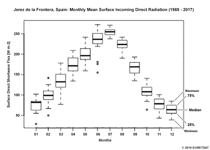
You understand how much land is needed to accommodate a sufficient number of solar panels to power the entire vineyard. However, the quantity of land needed is greater than the amount of land available on this particular farmer’s vineyard. In order to leverage what is available in the smaller plot of land, you must determine whether there is adequate solar radiation to power the solar panels during the grape growing season from June through September. You have analyzed a 30-year climate data record (CDR) from EUMETSAT's Satellite Application Facility on Climate Monitoring (CM SAF) of surface incoming direct radiation for the city.
Review the data plot and answer the questions in the carousel below. Click the arrows on the right and left side of the panel to navigate through the questions.
What other information can we learn from a CDR? Before we answer this question, let’s explore the various CDRs available and how we can obtain one from the CM SAF.
What is a Climate Data Record?
The CM SAF produces and archives satellite-derived climate data records (CDRs), a time series of measurements that are adequate in length, consistency, and continuity to determine climate variability. CDRs are used to support observations of the Earth system, such as studies of climate trends and variability and model verification to help improve climate models.
The CM SAF produces four types of CDRs: Environmental Data Records (EDRs), Interim Climate Data Records (ICDRs), Fundamental Climate Data Records (FCDRs), and Thematic Climate Data Records (TCDRs). Hover your cursor on the acronyms in the image below to learn more about each type of CDR.
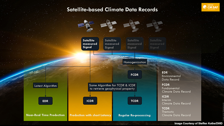
EDR - Time-tagged, Earth-located geophysical parameters produced from the satellite sensor data using the latest algorithms. These records are most suitable for studying the conditions at fixed times.
ICDR - A regularly updated TCDR available in short-time latency with an algorithm and processing system as consistent as possible to the generation of the corresponding TCDR.
TCDR - Geophysical variables derived from the FCDRs. An algorithm is applied to the FCDR to estimate the geophysical variable from the satellite observation. The production of a TCDR requires great time and computational resources, and it is usually updated every few years.
FCDR - Re-calibrated and inter-calibrated long-term data records of satellite radiance information. The need for recalibration results from the changes in the sensitivity of a satellite sensor during its operational orbit time. The need for inter-calibration results from technological advancements made in satellites and remote sensing sensitivity.
Question
For each task below, determine what type of climate data record (CDR) would work best to accomplish the task. Use the pull-down menu to choose the best answer.
The correct answers are highlighted above.
A FCDR is used by clients who want to independently retrieve a long time
series of radiance information or who want to assimilate these data into
their numerical weather prediction or climate models. FCDRs are well
suited for assimilation into climate models because these data are
calibrated and homogeneous in time.
A TCDR is the basis for all climate analysis or monitoring. As the TCDR
holds the geophysical variables derived from a calibrated and homogeneous
FCDR, it can be used to study climate trends.
In principle, an EDR should be the best product to use for geophysical
parameters during a recent time period, particularly if the retrieval
algorithm employs the full information of modern satellite instruments.
However, EDRs are not well suited for anomaly analyses or other
statistics that rely on consistent longer time series.
An ICDR may be used similarly to an EDR. However, ICDR and TCDR data can
be used together for climate analysis. For example, you can create an
anomaly by subtracting the long-term mean of a specific month (based on
TCDR) from the recent data of that month (based on ICDR), such as
October2019 minus mean(October1983to2015). Thus, the ICDR has an
advantage over the EDR in that it uses the same retrieval algorithm as
the corresponding TCDR and can be used for climate analysis.
The CM SAF provides CDRs for Essential Climate Variables (ECVs). ECVs are physical, chemical or biological variables (shown below) that play an important role in the Earth’s climate.
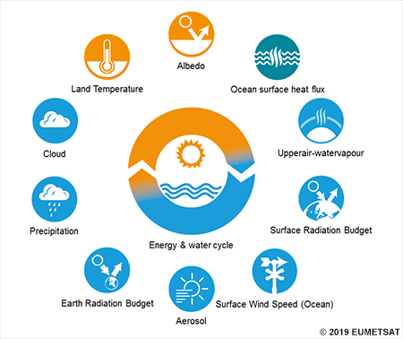
The primary variables covered by the CM SAF climate data records.
What is a Climate Data Record? » How Do I Get Data from the CM SAF?
Let's consider another scenario. Imagine you are working for the climate division in a National Meteorological and Hydrological Service (NMHS). Your main responsibility is to help gather and analyze climate information to support decision-making efforts. Where can you get climate data to help you provide decision-support services? The EUMETSAT's CM SAF is here to help!
To obtain a CDR from the CM SAF, follow the instructions below. You must click in the correct spot on the image in order to advance to the next step.
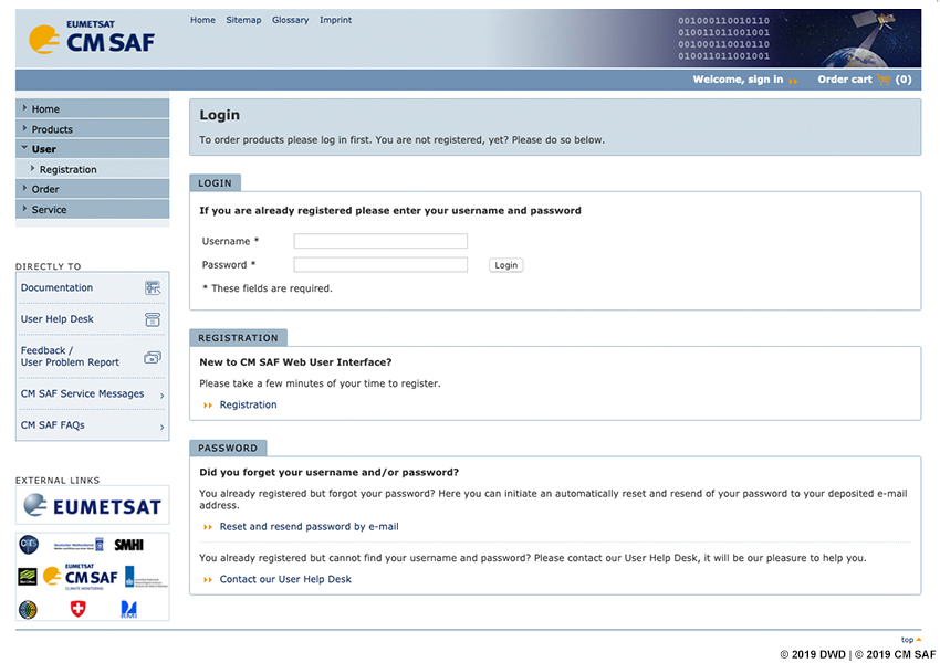
Step 1 of 9: Register
Go to EUMETSAT's CM SAF Login webpage and click on "Registration" under the "Registration" tab to create a user registration.
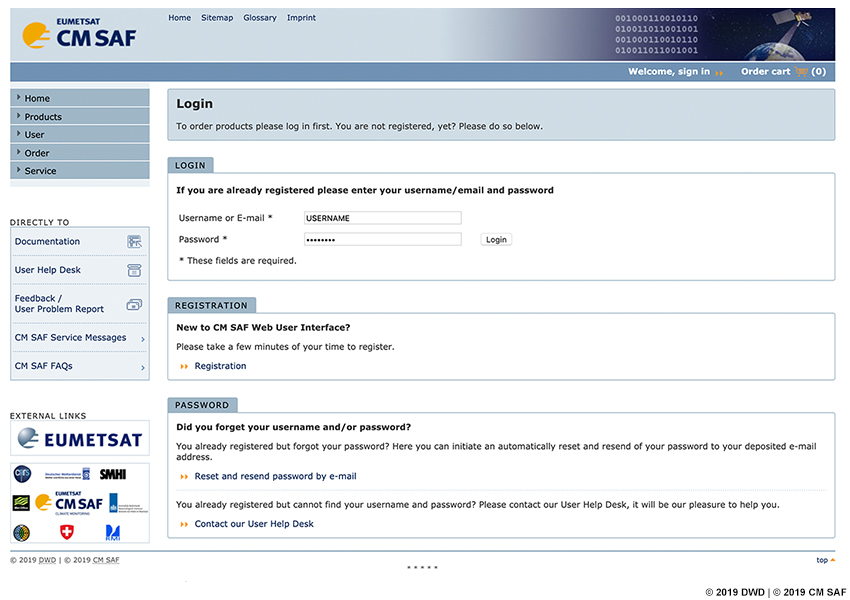
Step 2 of 9: Retrieve Login Details and Log In
An email will be sent to you from CM SAF Contact to confirm your registration and provide you with login details. On the Login page, type in your username or email associated with your account and password, and click “Login”.
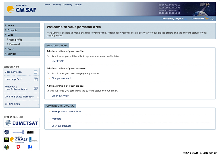
Step 3 of 9: Go to CM SAF - Product Navigator
Once signed in, navigate to the CM SAF - Product Navigator by clicking on the “Show product search form” under the “Continue Browsing” tab.
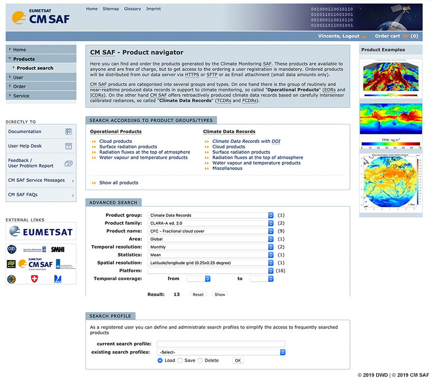
Step 4 of 9: Search for a CDR
On the CM SAF - Product Navigator Web User Interface (WUI), you can get a CDR by 1) “Searching According To Product Groups/Types" or 2) through an "Advanced Search". In this example, we will get a fractional cloud cover CDR through an Advanced Search. Use the pull-down menus to select your desired CDR characteristics. When you are ready, click “Show” to view the list of products that fit your criteria.
Tip: If you have a set criteria that you use frequently to find a particular CDR, you may name and save this criteria in the “Search Profile” tab (you must sign in to use this feature).
Note: The term "CDR" used in the CM SAF ordering page refers to "TCDR".
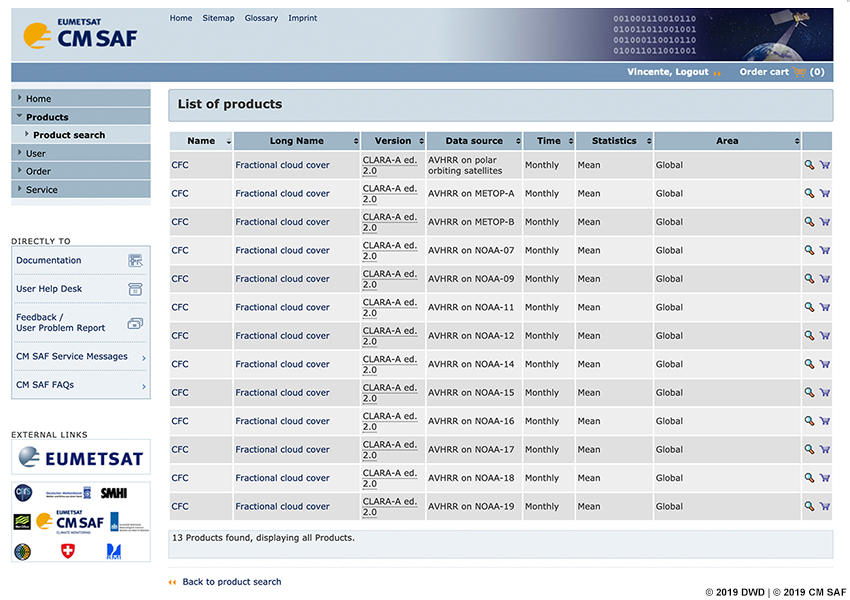
You can find your fractional cloud cover CDR in the “Search According To Product Groups/Types” tab by clicking on “Cloud Products” under the Climate Data Records section. The next page will show a List of Products based on that CDR group/type. You may alphabetically arrange any of the details in the columns to help you find your desired CDR by clicking on the up/down arrow to the right of the column title.
Step 5 of 9: Choose a CDR
From the List of Products page, you can view the details or directly order your desired CDR. In this case, we are interested in the first CDR at the top of the list, which has a combination of all available satellites and thus offers the best spatial coverage. Choose the first CDR by clicking on its name, long name, or magnifying glass.
Step 6 of 9: Review Product Details
From the Details of Product page, you can review the characteristics of your selected CDR, including product user manuals and algorithm documentation. When you are ready, click on “Add to order cart” to continue defining your CDR request.
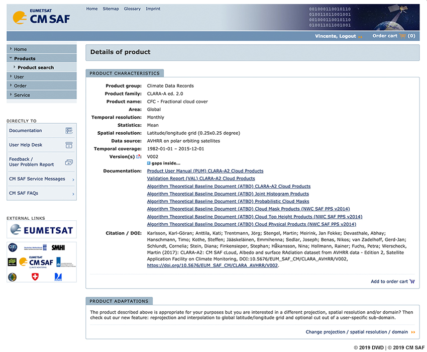
Tip: You may change the projection, spatial resolution, and domain of your CDR if desired. Such changes will restrict the domain to your region of interest and conveniently reduce the amount of data you will order and download. To do so, click on "Change projection/spatial resolution/domain" in the "Product Adaptation" tab. When you are done with your customization, click on "Proceed to Time Selection".
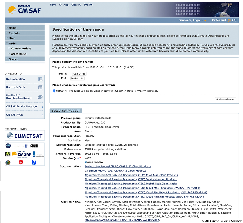
Step 7 of 9: Specify Time Range
From the Specification of Time Range page, define the desired time range for your CDR. The time range available from the record is displayed by default. When you are finished, click “Add to order cart”.
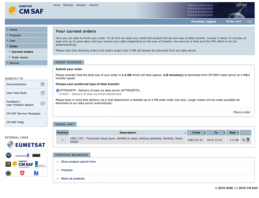
Step 8 of 9: Review and Place Order
On Your Current Orders page, choose your preferred type of data transfer and review your order cart. When you are ready to submit your order, click “Place an order”.
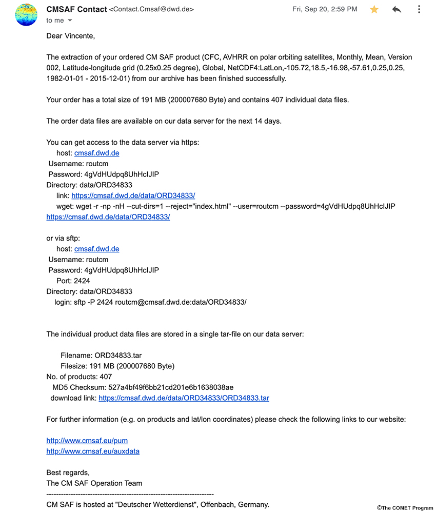
Step 9 of 9: Download Your CDR
The CM SAF thanks you for your order. An email from CM SAF Contact will be sent to you to confirm your product request information. Once CM SAF has processed your product request, an email will be sent to you from CM SAF Contact with instructions on how to access the data server to obtain your product(s). The individual product data file(s) are stored in a single tar-file on the CM SAF data server. If the order exceeds a size of 4.7 GB, you will get several tar-files with a max size of 4.7 GB.
Now you know how to get a CDR, but how can you visualize these data records? Let’s review the software packages needed to visualize CDRs from the CM SAF.
What is a Climate Data Record? » What Do I Need to Visualize a CDR?
What are the steps you need to take to get a CDR from the CM SAF? Click and drag the steps below into the correct order.
The correct order of steps needed to retrieve a CDR from the CM SAF is as follows:
- Register an account on the CM SAF website
- Sign into the CM SAF website
- Go to CM SAF - Product Navigator WUI and find your CDR
- Customize your CDR order if desired and add to your order cart
- Submit order and wait for email that states order processing is complete
- Review email for instructions to download your CDR
To review the steps for accessing and downloading a CDR from the CM SAF, please see the section “How Do I Get Data from the CM SAF?”.
The CM SAF provides different tools to work with CDRs, one of which is the CM SAF R Toolbox.
The CM SAF R Toolbox can prepare, analyze, and visualize CDRs in NetCDF format using the R programming language. To install the necessary software for the Toolbox on your operating system, please follow the instructions in the carousel below. Click on the right/left arrows to navigate through the steps.
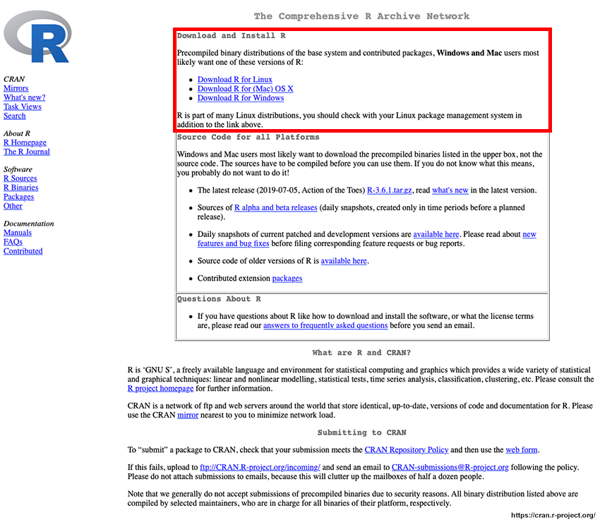
Step 1 of 6: Install R
Go to https://cran.r-project.org/ and follow the instructions to install R depending on your operating system (Version >= 3.5).
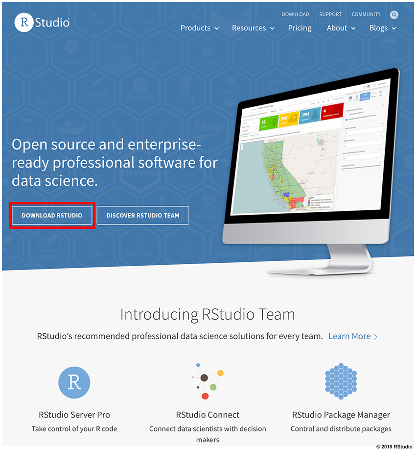
Step 2 of 6: Install RStudio
Go to www.rstudio.com and click on "Download RStudio". Follow the instructions to install RStudio Desktop depending on your operating system. It is recommended to work in RStudio when running the CM SAF R Toolbox because it is a user-friendly environment for R programming (but it is not required to run the Toolbox).
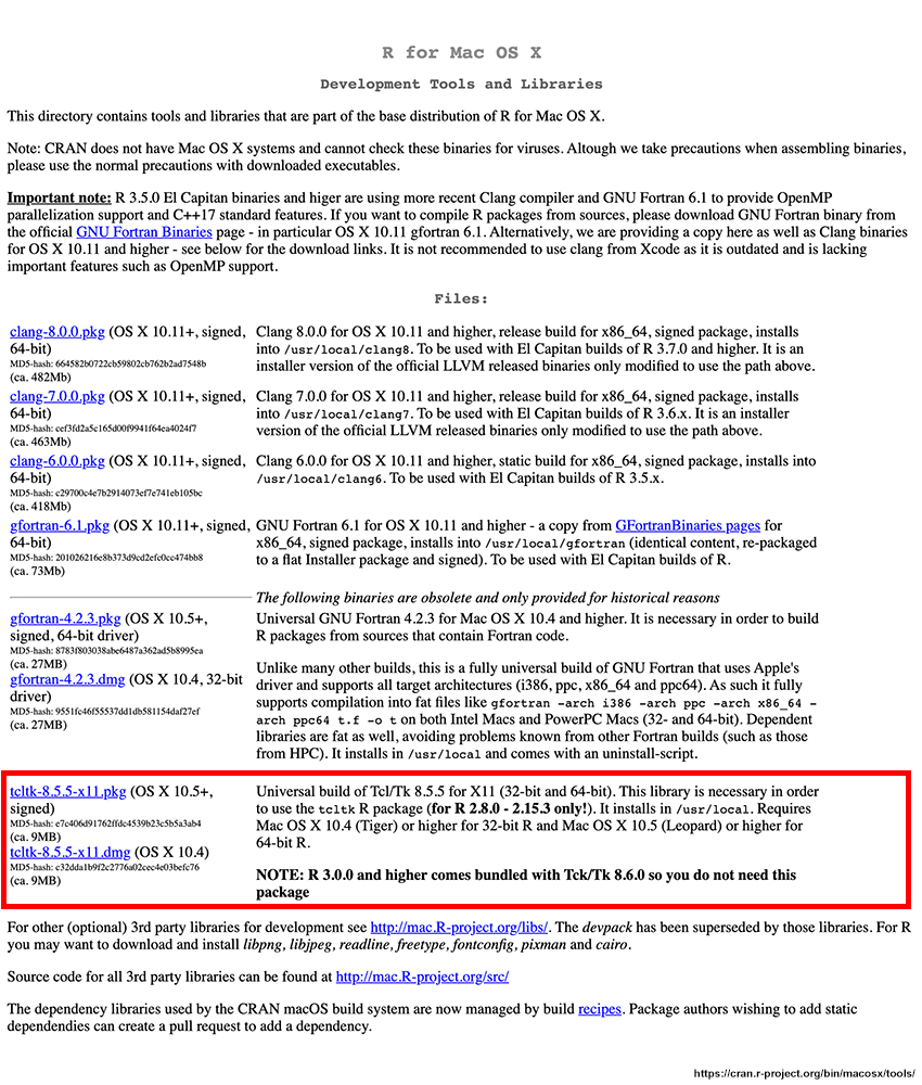
Step 3 of 6: Install Tcl/Tk package
For Mac OS X users only. If you are a Windows User, skip to Step 5.
Download the latest Tcl/Tk package available towards the bottom of the Development Tools and Libraries webpage. This package will be used to set up the directory where the output will be written as well as the resolution for your default grid (in the case of interpolation).
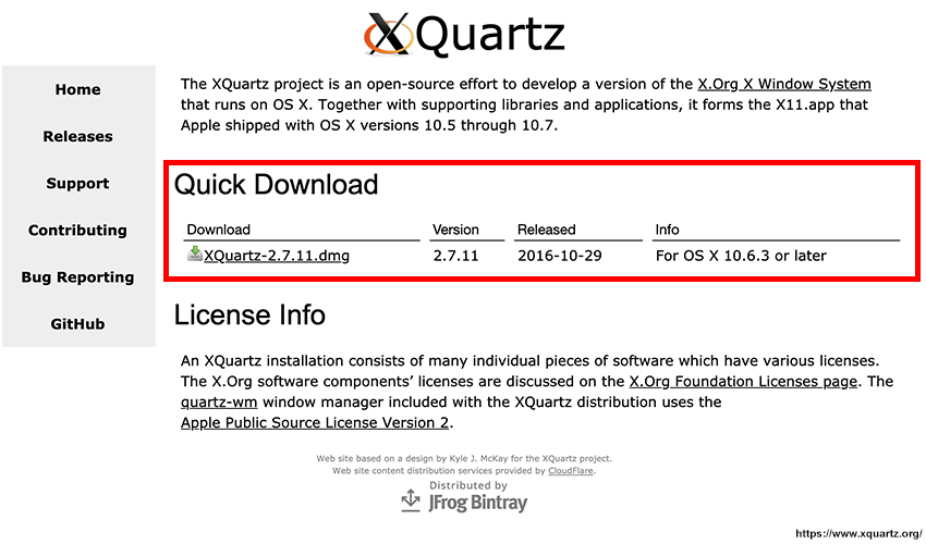
Step 4 of 6: Install XQuartz
For Mac OS X users only. If you are a Windows User, skip to Step 5.
Download the latest version of XQuartz at https://www.xquartz.org/
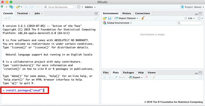
Step 5 of 6: Run the Toolbox
- In the RStudio console, execute the following command (shown in image
below):
install.packages(“cmsaf”) - Then, start the CM SAF R Toolbox by executing the following commands (not
shown in image below):
library(cmsaf)
run_toolbox()
Step 6 of 6: Set Up the Toolbox
Set up the CM SAF R Toolbox by a) choosing a user directory and b) specifying a grid resolution. Both steps are only done once during Toolbox set up. For more details, hover your cursor over each area identified by an arrow on the image below.
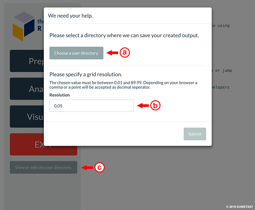
a) Choose a user directory on your computer. An output directory will be created in this folder in which all created NetCDF files will be stored.
b) Specify a grid resolution. In order to visualize data that is not provided on a rectangular longitude/latitude grid, the Toolbox will remap this data onto such a grid. The given value will determine its spatial resolution. Note that either a comma or period will be accepted as decimal separator dependent on what browser you are running the Toolbox in.
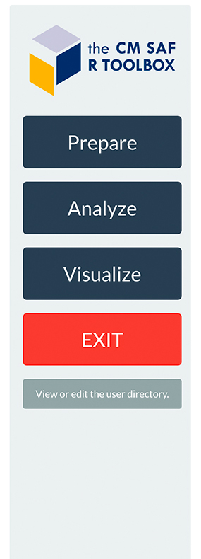
c) If you want to change the user directory at a later point, you can do so by clicking [View or edit the user directory.] on your Toolbox home screen.
The CM SAF R Toolbox is now ready for use!
Now that you know where you can get climate data, and the tools you need to visualize these data, what kinds of plots can you make? In the next section, we will learn how to analyze and generate various data plots using the CM SAF R Toolbox.
Using Toolbox to Help Install Observatory
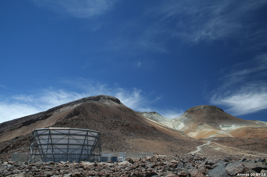
A picture of the Atacama Cosmology Telescope (ACT) in the Atacama Desert in Chile.
As a forecaster working in the climate division of an NMHS, you have been consulted by an astronomical society in South America interested in installing a high-altitude observatory site that would have unobstructed views of the horizon and less light pollution. In conversing with the astronomical society, you learned that cloud cover is an important factor in determining the quantity of time that is useful for an observatory. An average fractional cloud cover of 20% or less is the optimal condition needed for the installation project. You also learned that an ideal location for the site is at an elevation of at least 2000 m. At higher elevations, the Earth’s atmosphere is thinner and starlight appears less distorted in these conditions.
You want to generate a customized map that shows the mean fractional cloud cover across your domain. To begin your assessment, you want to download a CDR of monthly mean fractional cloud cover across South America based on the 34-year period from 1982 January 01 through 2015 December 01.
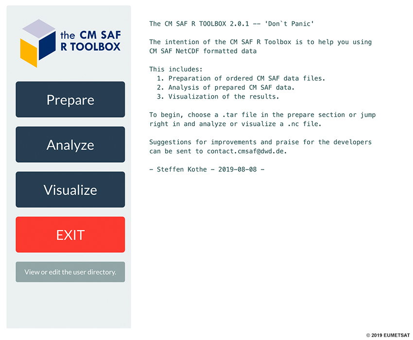
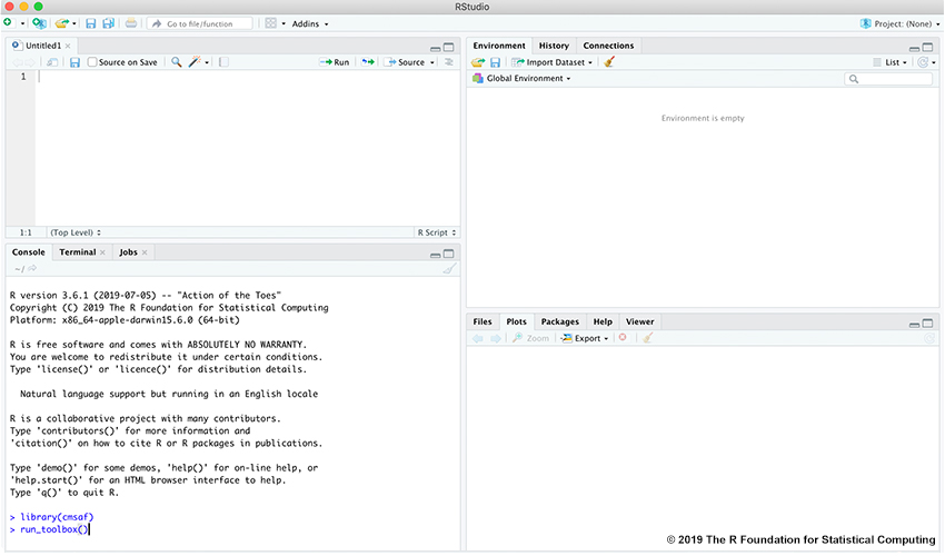
Let’s get the CM SAF R Toolbox up and running by opening RStudio and executing the following commands (shown in the image below):
library(cmsaf)
run_toolbox()
The carousel below will walk you through a series of steps in the CM SAF R Toolbox to prepare, analyze, and visualize your CDR. Click in the correct spot on the image, or click on the right/left arrows to navigate through the steps.
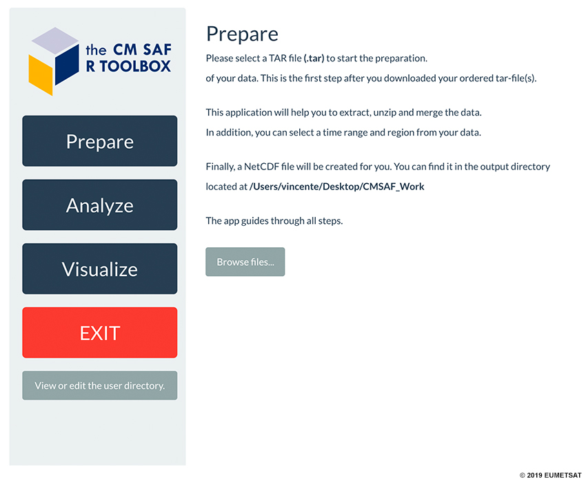
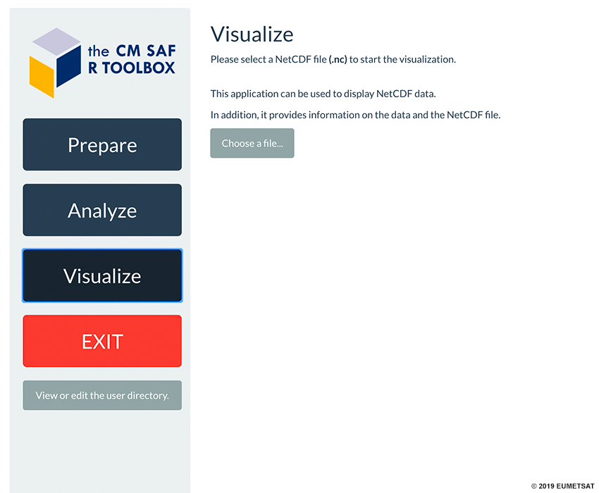
Step 1 of 7: Prepare the CDR
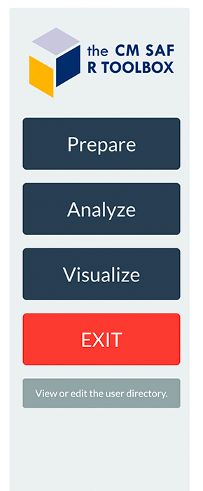
In the CM SAF R Toolbox interface, click "Prepare".
Step 2 of 7: Browse for .tar file
In "Prepare", click "Browse files..." and select the .tar file to begin the preparation of your data for analysis.
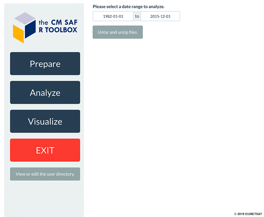
Step 3 of 7: Select Date Range
Once you have selected your downloaded .tar file, the Toolbox will merge all associated data files and extract the date range available to analyze. You can select a particular date range if desired. After selecting a date range, click "Untar and unzip data files". The Toolbox will begin untaring your data files.
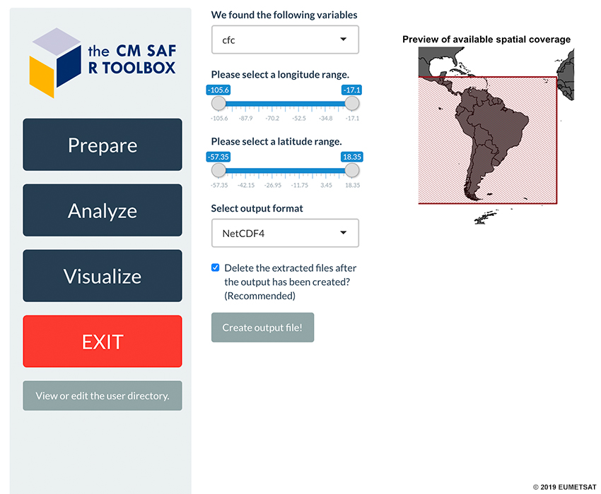
Step 4 of 7: Select Parameters for Output File
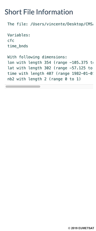
After untaring, you will be able to select the variable, latitude, longitude, and output format for your data file. When you are ready, click “Create output file!”. The final NetCDF output file will be placed in your designated output folder.
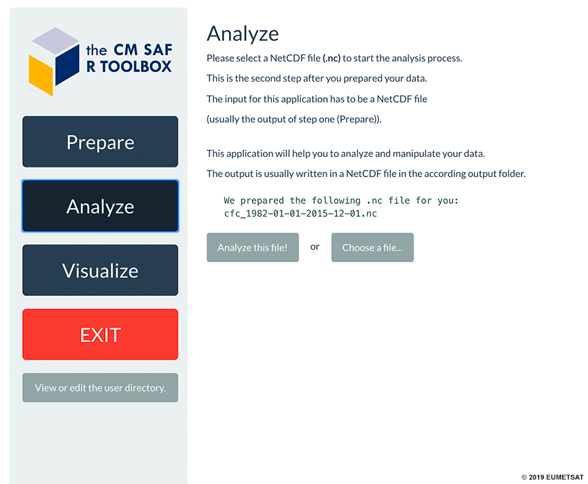
Step 5 of 7: Get Ready to Analyze the CDR
Once you have created your output file, the Toolbox will automatically direct you to analyze your data. The NetCDF file from the previous step is automatically chosen. Click “Analyze this file!” to initiate your data analysis.
It would be beneficial to gain insight into the fractional cloud cover across the region and determine the location that would be best suited for the high-altitude observatory. Your goal is to create a map from the CDR that shows the mean fractional cloud cover at each grid point across your domain of interest. Continue in the walkthrough to learn how to generate this map.
Step 6 of 7: Decide the Operator to Perform
- You can select the variable, group of operators, a particular operator, and the output format for your analyzed data file.
- To determine the mean fractional cloud cover in your data record (i.e., a
climatological mean), select the following options in the Toolbox:
- Please choose a variable: cfc
- Select a group of operators: Temporal operators
- Select an operator: All-time means
- To visualize the results after applying the operator, check the checkbox that reads “Do you want to visualize the results right away?”
- When you are ready, click "Apply operator". The Toolbox will apply the given operation(s), and the final analyzed NetCDF file will be placed in your designated output folder.
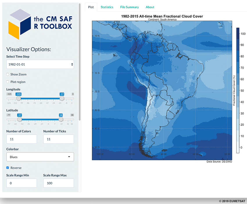
Step 7 of 7: Visualize, Customize, and Save Your Plot
- After applying operation(s), the Toolbox will immediately display your analyzed data.
- There will be several options to customize your data plot such as spatial extent, colorbars, titles, etc.
- To create a map of the all-time mean fractional cloud cover at each grid point
across our domain of interest, select the following options in the Toolbox:
- Number of Colors: 11
- Number of Ticks: 11
- Color bar: Blues
- Check box for “Reverse”
- Scale Range Min: 0
- Scale Range Max: 100
- Check box for “Plot Country Borders”
- Change title to “1982-2015 All-time Mean Fractional Cloud Cover”
- Change subtitle to “Continent: South America
- Once you have customized your plot, click "Save as png-file" to save your image (not shown below).
Question
To supplement your assessment of the mean fractional cloud cover across your domain, you decide to compare that data with the topography of South America.
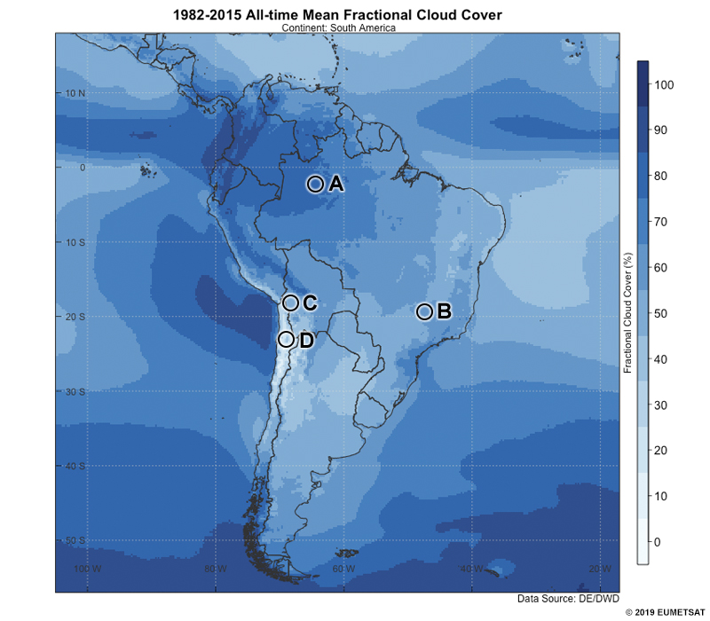
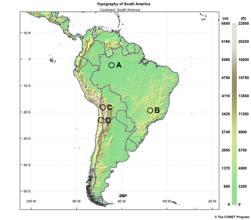
Based on the data plots above, which location would best serve an astronomical observatory? Choose the best answer.
The correct answer is d.
Location D (near 26 S, 70 W) is in an area that has a mean fractional cloud cover of about 10%. Based on this analysis of the CDR, location D is below the minimum threshold requirements for project feasibility. Also, the topographic map shows that location D is at an elevation of around 2000 meters, which will make this location more enticing.
After describing the location you determined was most suitable for the astronomical observatory, the astronomical society is now interested in the cloud cover throughout the year at that location. It is important to build the observatory site in a place that experiences minimal cloud cover because a small percentage of annual meteor shower activity is visible to observers in the southern hemisphere. Let’s generate a graph that would give you a sense of the fractional cloud cover throughout the year at the specific location.
Using Toolbox to Help Install Observatory » Time Series
You want to generate a customized time series of the multi-year monthly mean fractional cloud cover based on the 34-year observation record. The carousel below will walk you through a series of steps to generate this time series. Click in the correct spot on the image, or click the right/left arrows to navigate through the steps.
Step 1 of 4: Get Ready to Analyze the CDR
After you have clicked "Analyze" in the CM SAF R Toolbox and followed the instructions to retrieve your output file for analysis, click "Analyze this file!"
Step 2 of 4: Select Location Parameters
- To perform a data analysis at a particular location, select the following
options in the Toolbox:
- Please choose a variable: cfc
- Select a group of operators: Selection
- Select an operator: Select data at given point
- Select latitude point: -26 (26 S)
- Select longitude point: -70 (70 W)
- Check the checkbox that reads “Do you want to apply another operator afterwards?”
- When you are ready, click "Apply operator". The Toolbox will extract the data at our defined location and create a NetCDF file that holds this location-specific data in your designated output folder.
Step 3 of 4: Select Operation at Location
- To determine the multi-year monthly mean for our particular location, uncheck
the box that reads “Do you want to apply another operator afterwards?”. Then,
select the following options in the Toolbox:
- Please choose a variable: cfc
- Select a group of operators: Monthly statistics
- Select an operator: Multi-year monthly means
- Check the checkbox that reads “Do you want to visualize the results right away?”
- When you are ready, click "Apply operator". The Toolbox will apply the operator on the location-specific data file, and place a new NetCDF file in your designated output folder.
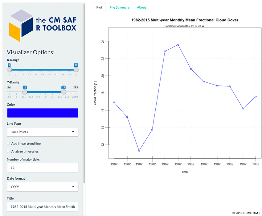
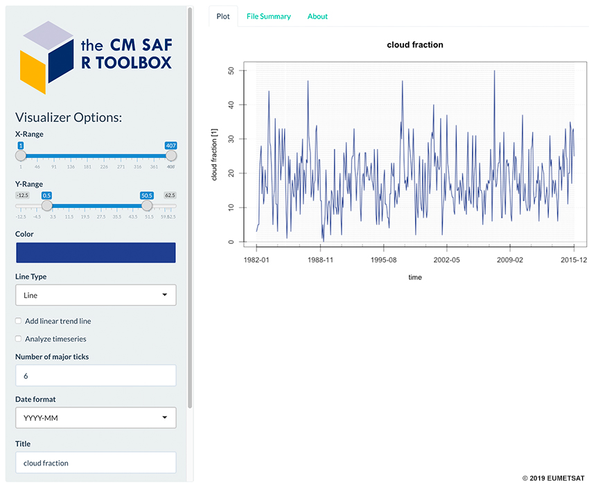
Step 4 of 4: Visualize, Customize, and Save Your Plot
When it is finished, the Toolbox will immediately display your analyzed location-specific data. Customize your plot, and click "Save as png-file" to save your image (not shown below).
Question
You have generated a customized graph that shows the multi-year monthly mean fractional cloud cover at the desired location for the high-altitude observatory.
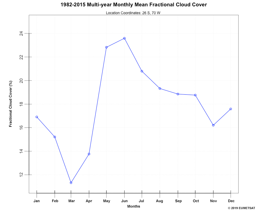
To maximize viewing conditions, the location should experience a monthly mean fractional cloud cover of no more than 20%. If the location has a history of not exceeding the monthly mean fractional cloud cover threshold for six months or more, the astronomical society will consider installing the high-altitude observatory. Review the graph above and answer the following questions. Use the pull-down menu to choose the best answer.
The correct answers are highlighted above.
In your assessment, you have determined that nine out of the twelve months at location D (near 26 S, 70 W) experienced a monthly mean fractional cloud cover of less than 20%. Based on this analysis, you have determined that this location is suitable for the installation of a high-altitude observatory.
Using Toolbox to Help Install Observatory » Analyze Time Series
The astronomical society has a few more questions before making their decision on whether to install the high-altitude observatory at location D (near 26 S, 70 W). The limited number of meteor showers that are best seen in the Southern Hemisphere occur during the winter/spring months of August, September, and October. The astronomical society is interested in the distribution of fractional cloud cover observations at that location during the winter/spring months to determine whether visibility would be optimal to observe the meteor showers during maximum activity.
Let’s generate a diagram that would give you a sense of the fractional cloud cover distribution throughout the year at the specific location. You want to generate a customized box-and-whisker diagram of the monthly mean fractional cloud cover based on the 34-year observation record. The carousel below will walk you through a series of steps to generate this diagram. You must click in the correct spot on the image in order to advance to the next step.
Step 1 of 3: Select Location-Specific Data File
After you have clicked on "Visualize" in the CM SAF R Toolbox, click “Choose a file” to select the location-specific data file you previously produced because it will already contain the monthly mean data for your location.
Step 2 of 3: Analyze Time Series
The Toolbox will immediately display the time series of your location-specific data. Check the box that reads "Analyze timeseries".
Step 3 of 3: Save Your Plot
A series of 6 plots will appear: time series, average seasonal cycle, monthly anomalies, box plot, annual means, and a histogram. Click "Save as png-file" to save your image (not shown below).
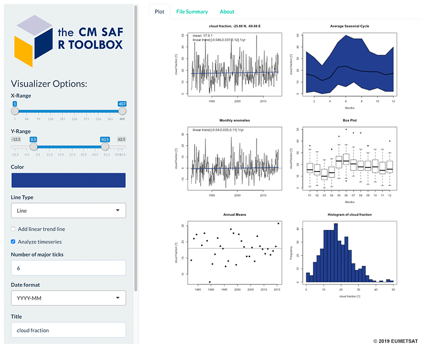
In this case, we will focus our attention to the box-and-whisker diagram.
Question
You have generated a customized box-and-whisker plot that shows the distribution of monthly mean fractional cloud cover at the desired location for the high-altitude observatory.
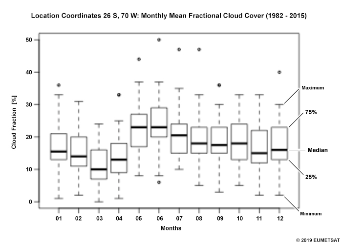
To maximize viewing conditions during the winter/spring months of August, September, and October, the fractional cloud cover at location D should be less than 25%. If 75% of the historical observations are below this threshold for a majority of those months, the astronomical society will consider installing a high-altitude observatory. Review the plot above and answer the following questions. Use the pull-down menu to choose the best answer.
The correct answers are highlighted above.
At this location, 75% of the observations in August, September, and October never exceed an average monthly mean fractional cloud cover of 25%. Based on this analysis, you have determined that a high-altitude observatory at this location is likely to experience minimal cloud cover to support meteor shower observation periods during the winter and spring.
After discussing your findings about the fractional cloud cover in South America and sharing your thoughts on installing the high-altitude observatory, the astronomical society are optimistic about their plans. You wish them luck in their pursuit of the installation and offer your services for future inquiries.
Now that you are familiar with the procedures for visualizing a CDR in different forms using the CM SAF R Toolbox, you decide to leverage the tool in your case study of the 2003 heat wave across Europe.
Using Toolbox to Revisit Heat Wave Event
What is the purpose of each tool below? Use the pull-down menu to choose the best answer.
The correct answers are highlighted above.
To review the tools needed to visualize CDRs, please see the section “What Do I Need to Visualize a CDR?”
You are revisiting case study data from a 2003 heat wave across Europe to learn about the characteristics that made this heat wave such a historic event. The heat wave began in June and lasted through mid-August of 2003. High temperatures and no precipitation dominated for an extended period of time. You begin with Germany, which saw excessive mortality rates in the month of August as a result of the heat wave.
You will be using the CM SAF R Toolbox to analyze the heat wave event based on the monthly sum of sunshine duration during a 33-year data period from 1983 January 01 to 2015 December 31. Review and answer the series of six questions in the carousel below to gain insight about the 2003 heat wave in Germany. You must answer each question in order to view the next in the series.
Question 1 of 6
If you execute the following options in the CM SAF R Toolbox, what kind of graphic should get produced? Choose the best answer.
- Select a group of operators: Monthly statistics
- Select an operator: Multi-year monthly means
- Select Time Step: August (displayed as 1983-08-01)
The correct answer is d.
Taking the steps above will create a climatological map of the multi-year monthly mean sum of sunshine duration across Germany in August. Continue to the next question to see the map and answer the question.
Question 2 of 6
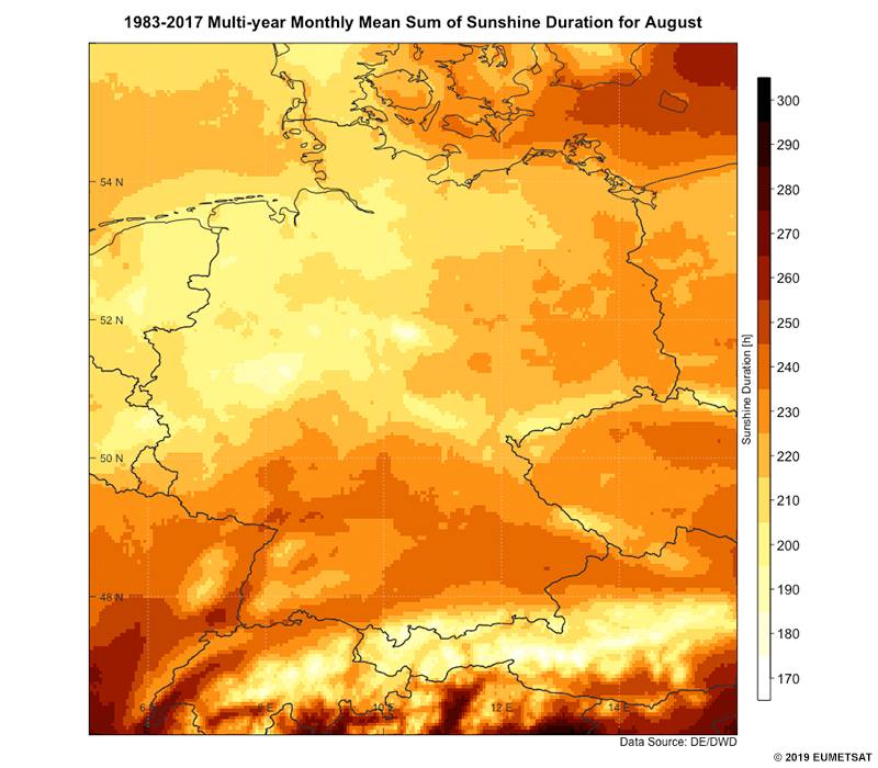
Which areas in Germany observed the greatest multi-year August mean sum of sunshine duration? Choose the best answer.
The correct answer is c.
Areas in southern Germany have observed a multi-year mean sum of sunshine duration between 235 and 245 hours in August, with a few local spots observing 245 - 255 hours.
Question 3 of 6
If you execute the following options in the CM SAF R Toolbox, what kind of graphic should get produced? Choose the best answer.
- Select a group of operators: Monthly statistics
- Select an operator: Monthly Anomalies
- Select Time Step: August in 2003 (displayed as 2003-08-01)
The correct answer is d.
Taking the steps above will create a climatological map across Germany that shows how anomalous the monthly sum of sunshine duration was in August 2003. Continue to the next question to see the map and answer the question.
Question 4 of 6
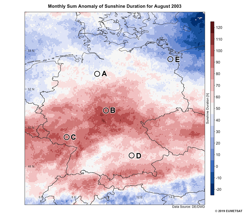
Which of the following locations in Germany shows the highest positive anomaly in sunshine duration for August in 2003? Choose the best answer.
The correct answer is b.
Location B exhibited the highest positive anomaly in sunshine duration for August 2003.
Question 5 of 6
If you execute the following options in the CM SAF R Toolbox, what kind of graphic should get produced? Choose the best answer.
- Initial Operation:
- Select a group of operators: Selection
- Select an operator: Select data at given point
- Select latitude point: 51
- Select longitude point: 10
- Check box for “Do you want to apply another operator afterwards?”
- Subsequent Operation:
- Select a group of operators: Selection
- Select an operator: Select list of months
- Please select months: June, July, August
- Check box for “Do you want to apply another operator afterwards?”
- Final Operation:
- Select a group of operators: Seasonal statistics
- Select an operator: Seasonal anomalies
- Uncheck box for “Do you want to apply another operator afterwards?”
- Check box for “Do you want to visualize the results right away?”
The correct answer is a.
Taking the steps above will create a climatological time series of the seasonal monthly sum anomalies of sunshine duration (hours) over the course of the data record at coordinate 51 N, 10 E, which is the city of Fulda, Germany. Continue to the next question to see the map and answer the question.
Question 6 of 6
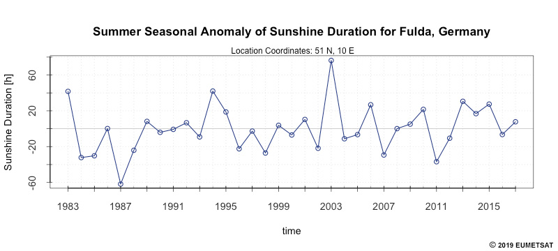
Which of the following statements is true regarding the 2003 heat wave based on the seasonal (JJA) monthly sum anomaly of sunshine duration in Fulda, Germany? Choose all that apply.
The correct answers are a, b.
The city of Fulda exhibited the greatest positive anomaly in sunshine duration during the JJA season in 2003. The sunshine duration was more than 60 hours above average!
Summary
In this lesson, we learned about the group of satellite-derived climate data records generated by EUMETSAT's Satellite Application Facility on Climate Monitoring (CM SAF): Environmental Data Records, Fundamental Climate Data Records, Thematic Climate Data Records, and Interim Climate Data Records. We reviewed the steps necessary to obtain a CDR using the CM SAF - Product Navigator Web User Interface, and gained an understanding of the software packages needed to visualize our data in the CM SAF R Toolbox: RStudio and the R Programming Language (with a couple of other packages for Mac OS X users).
To showcase CM SAF R Toolbox applications, the lesson provided an example of working with an astronomical society wanting to install an observatory in South America. The learner explored how to use the Toolbox to analyze a CDR of fractional cloud cover, interpreted the analysis, and shared the findings with the astronomical society. Finally, a quick overview of the 2003 European heat wave was provided to test the learner's understanding of using the CM SAF R Toolbox.
For more information on downloading and using the CM SAF R Toolbox, please see the following resources:
- CM SAF Climate Monitoring Homepage
- CM SAF R Toolbox: Installation and How-To-Use Materials
- Additional Installation Support
Contributors
COMET Sponsors
MetEd and the COMET® Program are a part of the University Corporation for Atmospheric Research's (UCAR's) Community Programs (UCP) and are sponsored by
- NOAA's National Weather Service
(NWS)
with additional funding by: - Bureau of Meteorology of Australia (BoM)
- Bureau of Reclamation, United States Department of the Interior
- European Organisation for the Exploitation of Meteorological Satellites (EUMETSAT)
- Meteorological Service of Canada (MSC)
- NOAA National Environmental Satellite, Data and Information Service (NESDIS)
- NOAA's National Geodetic Survey (NGS)
- National Science Foundation (NSF)
- Naval Meteorology and Oceanography Command (NMOC)
- U.S. Army Corps of Engineers (USACE)
To learn more about us, please visit the COMET website.
Project Contributors
Project Lead
- Vanessa Vincente — UCAR/COMET
Instructional Design
- Bryan Guarente — UCAR/COMET
- Tony Mancus — UCAR/COMET
Science Advisors
- Dr. Steffen Kothe — Deutscher Wetterdienst (DWD)
- Dr. Christine Traeger Chatterjee — EUMETSAT
- Dr. Jörg Trentmann — Deutscher Wetterdienst (DWD)
- Bryan Guarente — UCAR/COMET
Program Oversight
- Bryan Guarente — UCAR/COMET
Graphics/Animations
- Steve Deyo — UCAR/COMET
Multimedia Authoring/Interface Design
- Gary Pacheco — UCAR/COMET
COMET Staff, November 2019
Director's Office
- Dr. Elizabeth Mulvihill Page, Director
- Tim Alberta, Assistant Director Operations and IT
- Dr. Paul Kucera, Assistant Director International Programs
- Dr. Wendy Gram, Implementation Manager
Business Administration
- Lorrie Alberta, Administrator
- Auliya McCauley-Hartner, Administrative Assistant
- Tara Torres, Program Coordinator
IT Services
- Bob Bubon, Systems Administrator
- Joshua Hepp, Student Assistant
- Joey Rener, Software Engineer
- Malte Winkler, Software Engineer
Instructional Services
- Dr. Alan Bol, Instructional Designer/Scientist
- Tony Mancus, Instructional Designer
- Sarah Ross-Lazarov, Instructional Designer
- Tsvetomir Ross-Lazarov, Instructional Designer
International Programs
- David Russi, Translations Coordinator
- Martin Steinson, Project Manager
Production and Media Services
- Steve Deyo, Graphic and 3D Designer
- Jordan Goodridge, Student Assistant
- Dolores Kiessling, Software Engineer
- Gary Pacheco, Web Designer and Developer
Science Group
- Dr. William Bua, Meteorologist
- Patrick Dills, Meteorologist
- Bryan Guarente, Instructional Designer/Meteorologist
- Matthew Kelsch, Hydrometeorologist
- Andrea Smith, Meteorologist
- Amy Stevermer, Scientist/Instructional Designer
- Vanessa Vincente, Meteorologist