Introduction

High-Resolution Ensemble Forecast (HREF) systems are the next generation of ensemble prediction systems (EPS). HREFs use convection-allowing models (CAMs) to provide high-resolution probabilistic forecast information, including the location of mesoscale precipitation bands, and the probability of exceeding important temperature, precipitation, and wind thresholds at the scale of the HREF.

Many of you are familiar with using the Environmental Modleling Center (EMC) HREF from the National Centers for Environmental Prediction (NCEP) for severe weather guidance. In the cold season, however, different forecast problems arise. Snowfall and ice accretion rates depend on Quantitative Precipitation Forecasting (QPF) and the vertical structure of temperature and moisture. Frontogenetic forcing and conditional symmetric instability can result in heavy mesoscale precipitation bands. Precipitation type (ptype) forecasts are critical for assessing social and economic impacts of winter weather. Timing of ptype changeovers, precipitation onset, and precipitation conclusion are all important aspects of potentially high-impact winter weather.

For Impact-based Decision Support Services (IDSS), many emergency managers and other NWS core partners base decisions on specific thresholds for snow accumulation, temperature, and other weather elements. Probabilistic forecasts can help inform the likelihood that these thresholds are met; more so when the data is bias corrected. However, the best results are obtained when the probabilities are all calibrated to the verification probabilities. Presently, the forecast data in the HREF are only bias corrected, so the probability of exceedance should be used with caution.

You might ask, ”Since CAMs are so realistic, why not just use a single CAM forecast?” Just as in coarser-scale NWP, uncertainty comes into play. Model and initial condition imperfections increase forecast uncertainty in the timing, intensity, and location of winter weather features. HREFs allow you to quantify this inevitable forecast uncertainty and to assess the amount of confidence you should place in the forecasts for a potential winter weather event. In this lesson, you will see how to use and interpret HREF winter weather products to address these winter forecast problems.

This lesson includes the following sections:

• A description of the HREF produced at the EMC;
• The types of products currently provided for winter weather guidance;
• A case example where the probabilistic winter weather guidance is used in a winter storm situation

We will also provide web links to additional information on statistical methods used to produce the weather elements available from the HREF, including:

• Percentiles / Probability of Exceedance
• Conditional vs Unconditional Ptype Probability
• Point Probability / Neighborhood Probabilities / Ensemble Agreement Scale (EAS)

The EMC HREF

The EMC HREF » General Description

The EMC HREF was first developed in 2015 to provide probabilistic convective forecast guidance. With its capability to forecast mesoscale precipitation banding, topographically forced precipitation, and other terrain effects, the HREF can also provide useful probabilistic guidance for winter weather. The convection-allowing models (CAMs) used in the daily 00 and 12 UTC HREF cycles are shown in the graphic below, including the source for the initial conditions.

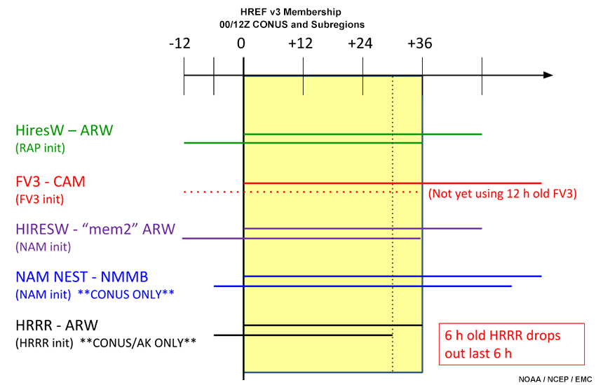
There are items several worth noting:

• As can be seen in the schematic, the HREF is a time-lagged ensemble. Its membership includes the two most recent runs of the five models indicated in the graphic. The lagged members are given less weight in computing ensemble mean quantities. Details for the current operational HREF (v2.1) are found in the MetEd Operational Model Encyclopedia under the Probabilistic Models link.
• As of summer 2019, the FV3 - CAM, while being used as an ensemble component, is not yet formally approved and implemented.
• EMC HREF version 3 (HREF v3) is expected to be made operational in Fall 2020.
• The National Weather Service Storm Prediction Center (SPC) independently runs an HREF with several of the same members and many of the same winter weather products.
• For the sake of simplicity, all future reference in this lesson to "HREF" refers to the EMC HREF v3.

The EMC HREF » High-Resolution Probabilistic Winter Products from HREF

The screen capture below shows the variables available from HREF. Variables in the blue boxes are directly or indirectly meaningful to winter weather forecasting.

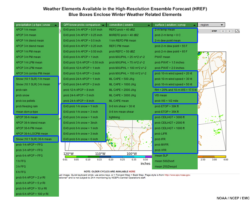
Along with ensemble-mean weather elements, the HREF has probabilistic products, including:

• Probabilistic ptype (not conditional; available in AWIPS)
• EAS neighborhood probability of exceedance for snowfall
• Probability (point) of exceedance for wind speed, ceilings, visibility < ½ mi, and temperature < 0°C (many available in AWIPS)

Application of Probabilistic Winter Weather Guidance

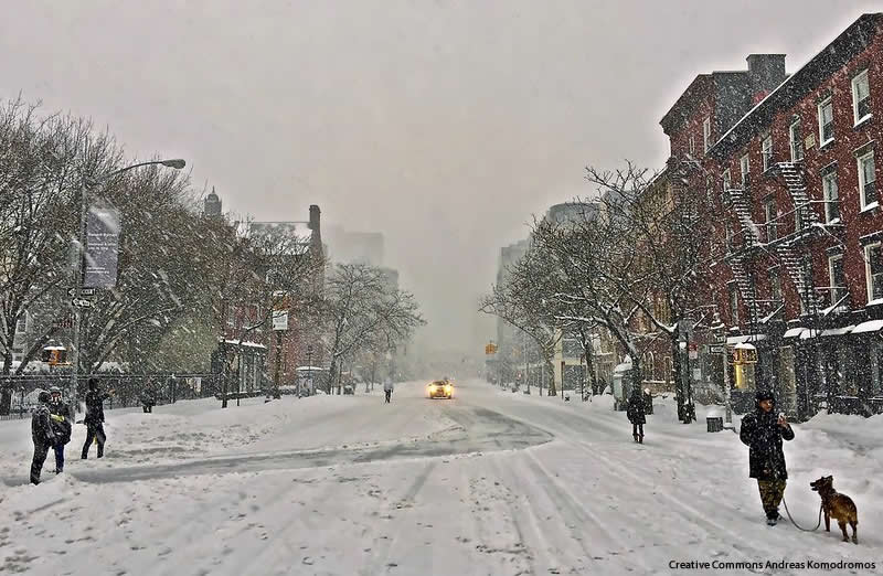
November 2018 was a chilly, wet month in the Northeastern U.S. On 15-16 November, an early season snowfall occurred that overperformed in accumulation and duration east of the Appalachian mountains because of a delay in an expected changeover from snow to rain. HREF v3 was available as a parallel version of the then-operational HREF to provide probabilistic winter weather guidance for days 1 and 2 (0 to 36 hours). In the next several sections, you’ll see examples of how to use the HREF probabilistic guidance for a series of forecast problems tied to this weather event.

Application of Probabilistic Winter Weather Guidance » Precipitation Type Determination and Transition

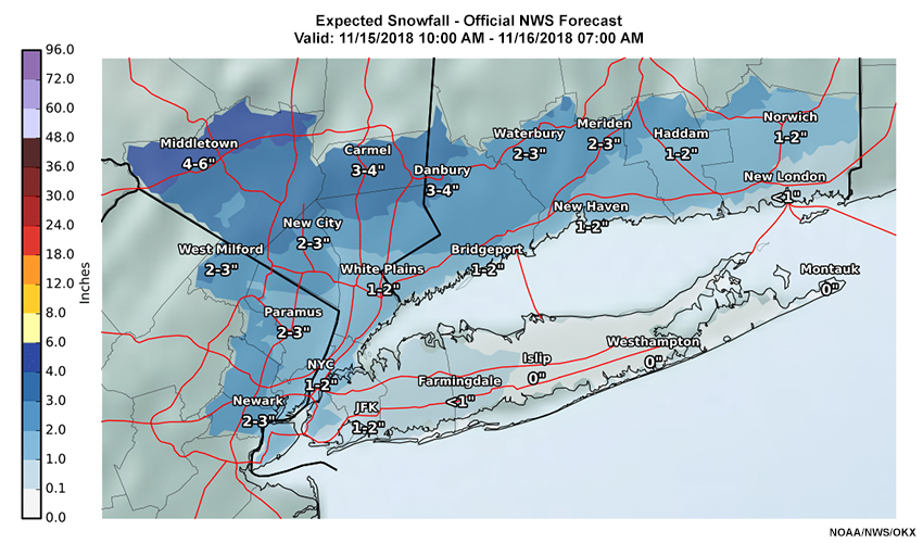
Forecaster Fran works as the Warning Coordination Meteorologist (WCM) at WFO New York, NY (OKX), serving the New York City area. As such, she is the focal point for communicating significant weather impacts to the jurisdictions in the county warning area (CWA). A map of the area of responsibility is shown below.

Fran is on the 14-15 November OKX overnight shift, and is monitoring the forecast for the upcoming day (15 November). As of early evening on 14 November 2018, the afternoon forecasters had issued winter weather advisories everywhere other than the New York City boroughs; Hudson County, NJ; and Long Island. Expected snow accumulations were less than 4” in the CWA and no winter storm watches or warnings were issued. The map below summarizes the CWA forecast of accumulations from 15 UTC 15 November through 12 UTC 16 November.

Application of Probabilistic Winter Weather Guidance » Precipitation Type Determination and Transition » Deterministic Guidance

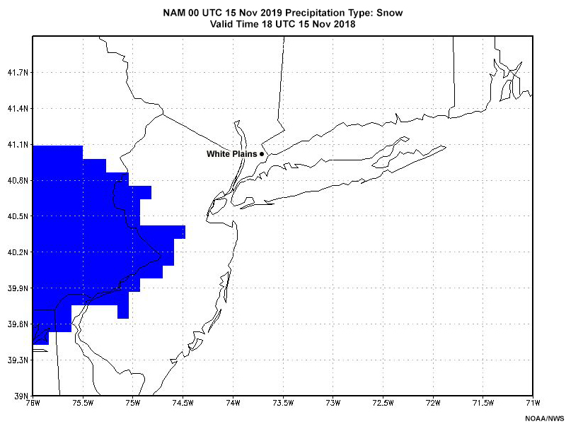
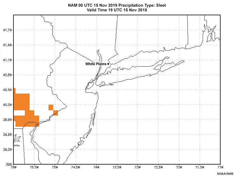
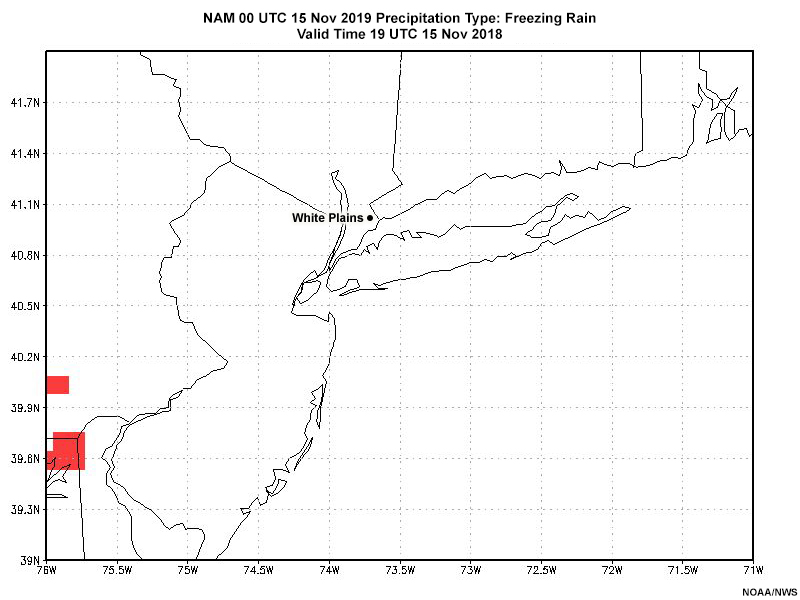
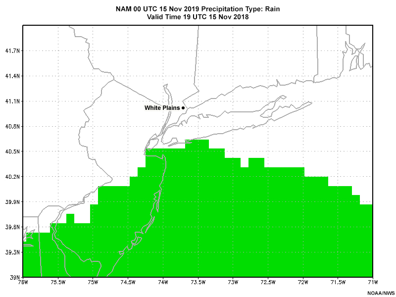
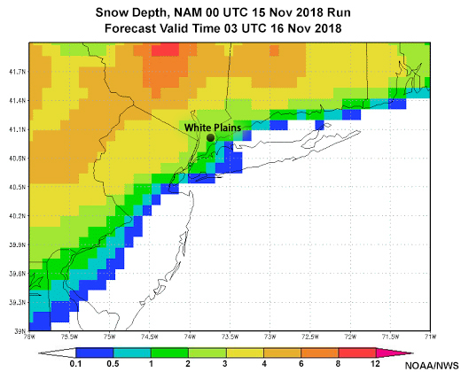
First, Fran wants to look at the deterministic guidance from the 00 UTC 15 November 12 km NAM (NAM12). Here’s what that guidance shows for the predominant ptype and snow accumulation for forecast valid times 19 UTC 15 Nov through 05 UTC 16 Nov.

Note the location of White Plains, NY. We’ll focus on this location for the remainder of this exercise.

• NAM Ptype Snow
• NAM Ptype Sleet
• NAM Ptype Freezing Rain
• NAM Ptype Rain
• Hourly Snowfall

NAM Ptype Snow

NAM Ptype Sleet

NAM Ptype Freezing Rain

NAM Ptype Rain

Hourly Snowfall

Question

Based on the NAM deterministic ptype and hourly change in snow depth (proxy for hourly snowfall), what would you conclude about snow accumulations between 21 UTC 15 November and 04 UTC 16 November in White Plains, NY?

a) There will be less than 1” of accumulation

b) There will be 1-3” of accumulation

c) There will be 2-4” of accumulation

d) There will be in excess of 4” of accumulation

The correct answer is b.

The hourly change in snow depth (a proxy for hourly snow accumulations) totals about 2”. This occurs between 20 and 00 UTC, with little accumulation thereafter.

Previously, the official forecast for snowfall in White Plains was for about 1” or so. Based on this single deterministic model, the prior forecast would need a small upward adjustment near White Plains, NY.

The total forecast snow depth according to the NAM by 03 UTC 16 November is shown below, and is in general agreement with the sum of hourly amounts around White Plains, NY.

From the graphic, Fran sees a steep snow accumulation gradient bisecting the OKX CWA. This implies that a small error in the forecast could result in significantly different impacts, especially given the timing of the event from early afternoon through the evening rush. Given the early time of year and the potential QPF from this storm, Fran decides she will examine the high-resolution HREF probabilistic guidance when it becomes available in an hour or two.

Please make a selection.

Application of Probabilistic Winter Weather Guidance » Precipitation Type Determination and Transition » Probabilistic Guidance - Precipitation Type

The HREF 00 UTC 15 November 2018 probabilistic guidance posts to the EMC website as expected. Fran checks where the NAM deterministic guidance falls with respect to the HREF probabilistic guidance. She reviews its ensemble mean and probabilistic guidance, keeping in mind the chances of high impact conditions and the potential need for IDSS as she considers the forecast problems associated with a winter storm.

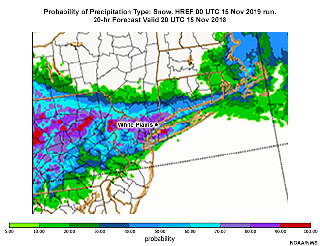
Fran examines the ptype point probabilities from the HREF run for snow, sleet, freezing rain, and rain. These are all displayed in tabs below. After reviewing these probabilities, answer the question that follows.

• Prob Snow
• Prob Sleet
• Prob ZR
• Prob Rain

Prob Snow

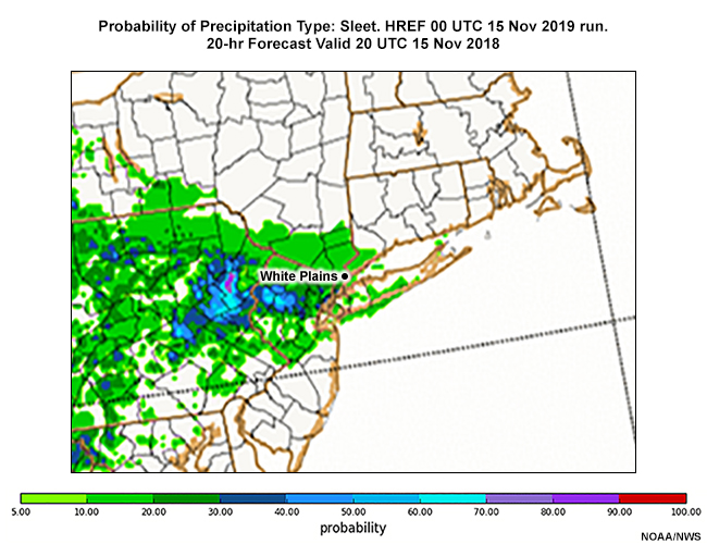
Prob Sleet

Prob ZR

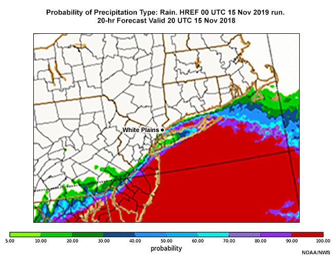
Prob Rain

Unsure of what this product is showing? See Conditional vs Unconditional Ptype Probability

For White Plains NY, (WP on maps) select the probabilities for each ptype at 21 UTC 15 November and again at 00 UTC 16 November 2018.

Application of Probabilistic Winter Weather Guidance » Precipitation Type Determination and Transition » Probabilistic Guidance - Ptype Changeover

• Prob Snow
• Prob Sleet
• Prob ZR
• Prob Rain

Prob Snow

Unsure of what this product is showing? See Conditional vs Unconditional Ptype Probability

Prob Sleet

Unsure of what this product is showing? See Conditional vs Unconditional Ptype Probability

Prob ZR

Unsure of what this product is showing? See Conditional vs Unconditional Ptype Probability

Prob Rain

Unsure of what this product is showing? See Conditional vs Unconditional Ptype Probability

“As the saying goes,'' Fran thinks, “timing is everything, and so is location. Evening rush hour in the metropolitan area generally runs from about 3 p.m. to 9 p.m. local time (20 UTC to 02 UTC). To better brief the local emergency managers, I need to check out when the precipitation changeovers will take place.”

Application of Probabilistic Winter Weather Guidance » Accumulating Snowfall

To address the uncertainty introduced in the deterministic forecast by the snow accumulation gradient, Fran looks for the exceedance probability data. The HREF provides Ensemble Agreement Scale neighborhood probability of exceedance maps for:

• 1 inch accumulations over a 1-hour period,
• 1 and 3 inch accumulations over a 3-hour period, and
• 1, 3, and 6 inch accumulations over a 6-hour period.

Fran decides to use the 6-hour probability of exceedance for the 1”, 3”, and 6” thresholds for the OKX CWA valid at 03 UTC to guide her decisions on snow accumulation updates for tomorrow’s evening rush. Forecasts valid at 03 UTC (10 p.m. local time) from the 00 UTC 15 November forecast runs are found in the tabs below. The maps below are zoomed in to the OKX CWA to provide more detail. Review those forecasts, then answer the question that follows.

• EAS Prob 6-hr Snow > 1”
• EAS Prob 6-hr Snow > 3”
• EAS Prob 6-hr Snow > 6”

EAS Prob 6-hr Snow > 1”

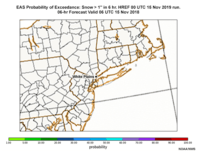
Unsure of what this product is showing? See Probability of Exceedance and Point, Neighborhood, and EAS Probability

EAS Prob 6-hr Snow > 3”

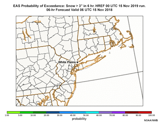
Unsure of what this product is showing? See Probability of Exceedance and Point, Neighborhood, and EAS Probability

EAS Prob 6-hr Snow > 6”

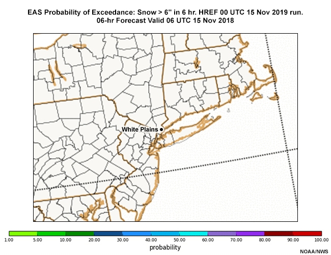
Unsure of what this product is showing? See Probability of Exceedance and Point, Neighborhood, and EAS Probability

Application of Probabilistic Winter Weather Guidance » Accumulating Snowfall » Forecast Implications

ERROR #6b: Graphic completion status for fileID=70572 is needs review. To access the MSDB for the image go here: 70572

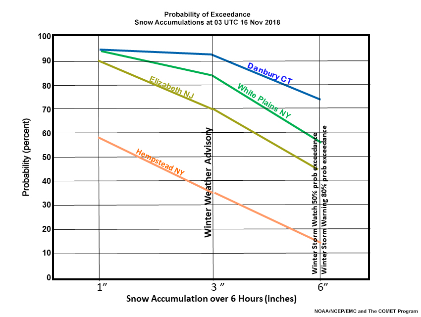
Fran plots the probability of exceedance distributions from this data to make it easier to visualize. The resulting graph is shown above. She then decides she has enough probabilistic forecast information to draw conclusions about possible storm scenarios, particularly for the evening rush hour (3 p.m. to 9 p.m. or 20 to 02 UTC).

First, she compares the probabilistic HREF forecast to the deterministic NAM forecast she reviewed earlier to see where it is in the full ensemble distribution.

Question

Recall that the total snow accumulation in the deterministic NAM12 from 00 UTC 15 November 2018 was about 2” in White Plains, NY, before the changeover to rain at about 01-02 UTC 16 November. At 03 UTC 16 November 2018, what is the approximate forecast probability of exceeding the 2” forecast based on the HREF range of forecasts? Choose the best answer.

a) It has a 15% probability of being exceeded

b) It has a 35% probability of being exceeded

c) It has a 50% probability of being exceeded

d) It has an 90% probability of being exceeded

The correct answer is d.

ERROR #6b: Graphic completion status for fileID=70573 is needs revision. To access the MSDB for the image go here: 70573

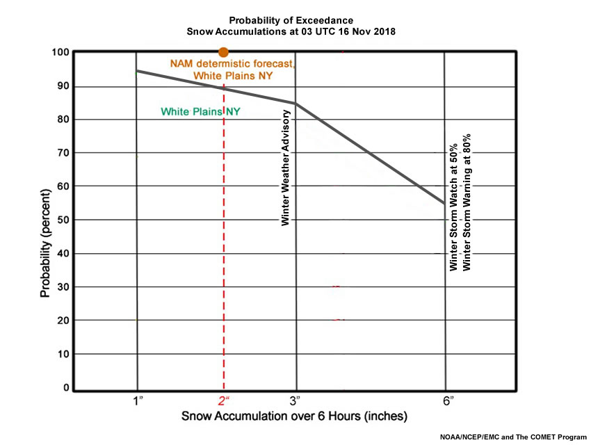
Fran placed the 2” value from the deterministic NAM forecast on the probability of exceedance diagram she prepared earlier. The 2” value intersects the White Plains NY probability of exceedance curve at ~90%, indicating a ~90% probability of exceeding 2”. Note also that the probability of exceedance at the winter storm threshold of 6” is 55%.

Please make a selection.

The HREF accumulates snow and sleet using a 10:1 snow-to-liquid-ratio (SLR), while the observed SLR for sleet is typically around 2:1 to 3:1. Therefore, Fran would be prudent to recheck how much sleet is included as a ptype especially in mixed precipitation situations such as this one.

There is only a slight chance of sleet before 00 UTC, Fran recalls. But sleet probabilities increase to about 40% before rain completely takes over by 03 UTC. Fran may consider reducing the HREF probability of accumulations exceeding 1”, 3”, and 6” because:

• There will be some minor amounts of sleet after 00 UTC that will slightly cut down accumulations;
• Climatologically, snow amounts of this magnitude are rare in mid-November.

Application of Probabilistic Winter Weather Guidance » Guidance for Watches, Advisories, and Warnings

Fran now has to decide how to modify the forecast. She looks again at the HREF snow exceedance probabilities she previously plotted.

ERROR #6b: Graphic completion status for fileID=70572 is needs review. To access the MSDB for the image go here: 70572

Application of Probabilistic Winter Weather Guidance » Verification

The accumulated snowfall as of 09 UTC 16 November 2018, is shown in the map from the New York, NY WFO below.

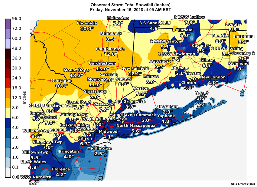
Summarizing the forecast versus observations:

• Underforecasting of snow was mostly the result of heavy initial snowfall rates (up to 2” or more per hour) and a delay in snow changing to rain in places along the coast (e.g., Long Island, NYC, eastern NJ, southern CT).
• New York City’s Central Park, with records from 1869 to the present, had its earliest 6” snowfall on record. Many other locations in the area broke early season records.
• The HREF was more useful as its range of forecasts captured the heavier than expected snowfall in most of the CWA. The area generally received snow amounts toward the high end of what was expected, in line with the high end of the HREF forecast.

Application of Probabilistic Winter Weather Guidance » Case Summary

This lesson walks the student through an early season snowstorm as it moved through the New York City area. The case study includes using the HREF products to assess start and precipitation changeover times, a rough range of snow accumulations over the evening rush hour, and the subsequent verification. It is demonstrated that, at least in this case, the HREF allowed for more helpful guidance by providing a “heads up” that high impact snow accumulations were possible in areas south of the deterministic guidance.

Important Statistical Concepts

Important Statistical Concepts » Probability of Exceedance

Probability of exceedance (PE) guidance quantifies the forecast risk that some critical meteorological threshold will be crossed. PE is determined by using a cumulative distribution function (CDF). The source of the CDF can be either empirical (defined directly by the data) or based on an expected distribution that best fits the data sample.

PE is used at critical thresholds for temperature, precipitation, or wind. In the cold season, PE is generally used for winter storms, heavy snow, winter weather advisories, ice accumulation, winds, temperatures (below freezing and below zero), and wind chill.

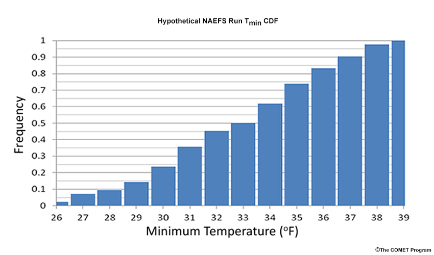
An example of such a CDF is shown below. Examine it and, recalling the definition of probability of exceedance, answer the question that follows.

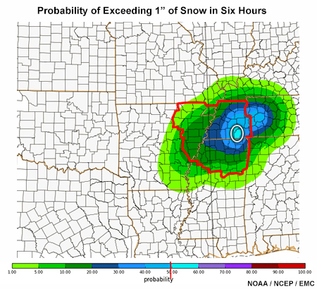
The probability of exceedance for some threshold value can be plotted on a map for any winter weather element at every grid point. Such guidance can be used to determine if winter storm warnings or winter weather advisories are needed.

Question

Assume a 50% probability of more than 1” over six hours is required for winter weather advisory issuance in the Memphis TN CWA (enclosed by the red boundary), and that no snow is expected before or after this six-hour period. Using the black pen below the diagram,

Circle the portion of the Memphis TN CWA that meets the threshold for a winter weather advisory.

Only a small area in the east-central part of the Memphis TN CWA meets the criteria for a winter weather advisory. That area is enclosed by a white oval in the graphic below.

Important Statistical Concepts » Conditional vs Unconditional Ptype Probability Example

Suppose we have a 20-member ensemble. The forecast at some time has a probability of precipitation of 60%. Thus 12 members show some precipitation, while 8 others do not. Now suppose that the members that show precipitation have a variety of precipitation types, including rain, sleet, and snow. We might end up with a distribution like this:

The conditional probability of rain states that if there is precipitation, what is the probability of rain (versus freezing rain, sleet, or snow), whereas the unconditional probability of rain says that regardless of whether there is precipitation or not, what is the probability of rain.

Important Statistical Concepts » Point, Neighborhood, and EAS Probability

Important Statistical Concepts » Point, Neighborhood, and EAS Probability » Point Probability

In probability, an event is a subset of outcomes that meet a requirement (e.g., winds exceeding 35 kt at a single location), to which a probability may be assigned. In an ensemble prediction system, the most simple probability is the number of ensemble members containing an event at some grid point.

The table below shows a wind forecast for a single point for an ensemble with 10 members.

Important Statistical Concepts » Point, Neighborhood, and EAS Probability » Neighborhood Probability

Mesoscale weather systems frequently exhibit uncertainty in location. For example you may be expecting scattered convection, but you don’t know exactly where the convection will set up. One way to account for this uncertainty is to look to the area surrounding a grid box for occurrences of an event of interest. If the area around the grid box has a fixed radius of 40 km, then you could account for the probability of an event (e.g., measurable precipitation) within 40 km of that grid box. A neighborhood probability is one way to do this. You’ll find a schematic of the neighborhood probability method below.

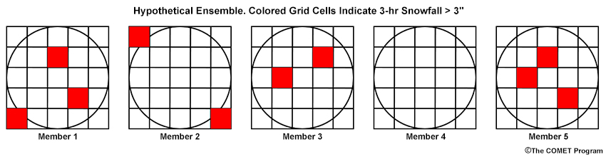
Suppose, for example, that you expect heavy banded snow one afternoon, with snowfall exceeding three inches in three hours. This defines our event. The neighborhood is an area around each grid cell with a defined radius, typically 40 km. Given a 5-member ensemble, if a member has a grid cell that meets our event criteria, snowfall exceeding three inches in three hours, anywhere in the neighborhood, then that is a positive match. In the example shown above, the circle is the neighborhood. Red grid cells indicate 3-hr snowfall > 3 inches. If 3 of the 5 members meet this criteria, as shown here, then we say the neighborhood probability is 3/5 = 60%.

Important Statistical Concepts » Point, Neighborhood, and EAS Probability » Fractional Coverage and the Ensemble Agreement Scale (EAS)

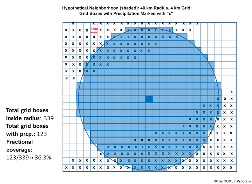
In this graphic example we see two hypothetical bands of precipitation denoted by “x”s, north and south of the neighborhood's central grid box in darker blue. Precipitation occurs in 123 of the 339 grid cells within 40 km of our grid cell. And thus we say that there is a 123/339 = 36% probability of precipitation within 40 km of this grid box. We call this fractional coverage. It acts to smooth the probability contours.

A variant of the fractional coverage metric is the Ensemble Agreement Scale (EAS). It’s similar to fractional coverage, but uses a full ensemble and a variable radius. Where the difference between ensemble members is small, the radius is small. As the difference between ensemble members increases, the size of the radius similarly increases. The EAS probability seeks to preserve information about the confidence in location when ensemble members agree. This method can be particularly useful in cases of orographic or coastally influenced weather. The EAS probability tends to preserve features associated with terrain and coasts that might otherwise be smoothed out.

How does this work in practice? Starting with a radius of one grid cell around a point, the similarity of the ensemble members is computed. If they are sufficiently similar, then the probability for that radius is calculated. If not, then the radius is increased to 2 grid cells and the similarity of the ensemble members is computed and evaluated for the expanded area. This process is repeated until the smallest radius is found that satisfies the similarity criteria (the ensemble agreement scale). A fractional coverage probability is then calculated for that radius (Blake et al., 2018).

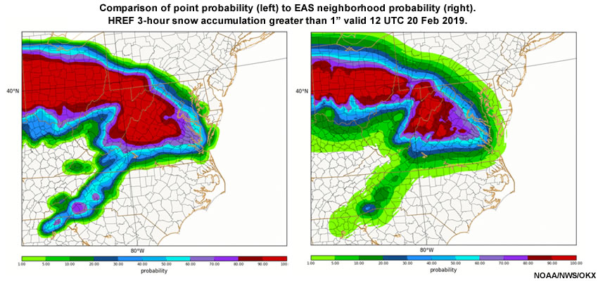
Compare point probability with an EAS probability plot for 3-hour snow accumulation greater than 1” and then answer the question that follows.

Summary

This lesson demonstrates the use of HREF probabilistic guidance in an early season snowstorm that struck the New York City area. In this case, the probabilistic guidance outperformed deterministic guidance from the NAM, pointing to a solution with a later changeover from snow to rain that contributed to higher snow accumulations than in the deterministic forecast.

HREF forecast products use a variety of statistical methods including conditional and unconditional probability of ptype and point and EAS neighborhood probability of exceedance. While unconditional probability includes all weather types in computing the chance of a precipitation type, conditional probability only includes ensemble members with precipitation only. This provides forecasters, emergency managers and other end users with risk assessment information under a narrower set of conditions. The probability of ptype allows forecasters and end users to assess the impact of a possible winter weather event based on the timing of winter precipitation onset and ptype changeovers.

The neighborhood methods measure the risk of exceeding critical thresholds for accumulating snow and ice. This helps both with assessing the need for winter weather watches, warnings, and advisories, and the confidence that the forecaster may place in the HREF probability of exceedance forecasts. The EAS methodology adapts to the amount of agreement among the HREF ensemble membership, which arguably makes EAS the best tool for both probabilistic forecasts and IDSS.

Contributors