1.0 Introduction
Sudden whiteout conditions with road icing along narrow corridors, motorists and air traffic are suddenly at risk. And if lake-effect snow is involved, rapid and heavy snow accumulation can close roads and paralyze cities. It’s a snow squall!
Are you using all the weather products that can help you forecast and track snow squalls? Accurate and timely forecast and monitoring information can help mitigate the impacts from squalls and may even make the difference between life and death. On 18 December 2019, a winter-weather system moved through central Pennsylvania, causing a series of snow squalls and life-threatening icing on highways and other thoroughfares.
In this lesson, we'll focus on this case and introduce some satellite products that can provide useful information about snow squall events.
Answer the four questions below. Use the arrows to navigate between them.
1.0 Introduction » 1.1 Conceptual Model
Based on many observations of snow squalls, Banacos et al. 2019 developed a snow squall conceptual model that summarizes key features and ingredients.
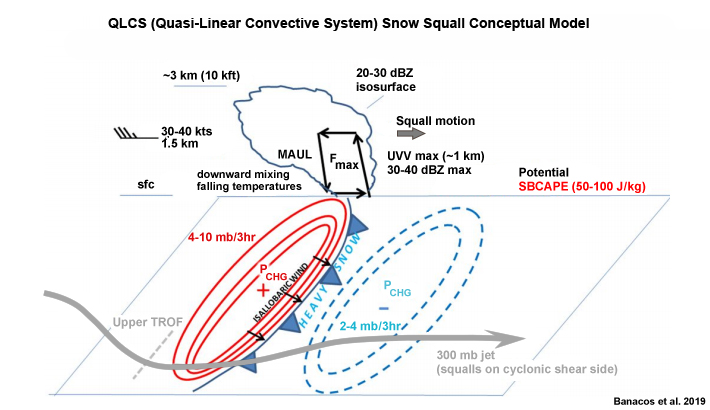
Observational datasets such as high-resolution satellite imagery can help identify some of these snow squall dynamics as they occur during a weather event. Throughout this lesson, we will highlight connections between this conceptual model and the observations in the 18 December case.
2.0 Synoptic Analysis - 12z Model Guidance
As 18 December began in central Pennsylvania, model guidance suggested that it would be a pretty active day, with the potential for scattered convection along and in advance of an Arctic cold front moving into the region from Ontario and Quebec.
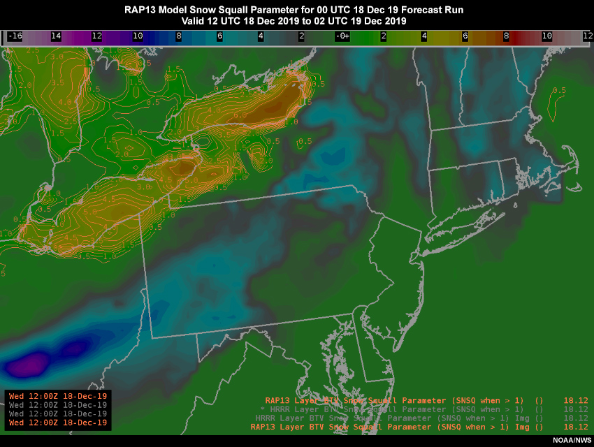
First, let’s take a look at the snow squall parameter loop from the 12 UTC (8 EST) run of the RAP13 forecast model.
Question
What does this loop indicate?
The correct answer is a.
Similar to the warm-season super-cell parameter used to predict supercell motion, the snow squall parameter is a multiple ingredient, composite index for indicating the potential for snow squall activity and is based largely on the QCLS snow squall conceptual model. Driven by model output, the parameter incorporates some of the best indicators of snowfall potential, including the orthogonal component of the low-level wind relative to a developing convective line or front, the magnitude of instability, and the amount of available lift, among others. Values exceeding 1.0 point to a favorable environment for snow squall development.
The animation shows favorable snow squall conditions beginning over lakes Erie and Ontario in the early morning. These conditions quickly spread into western PA and NY by mid-morning, and continue to intensify and spread eastward into the afternoon hours.
If you’re interested in viewing high resolution ensemble model output from a bit later in the morning, click the panel below.
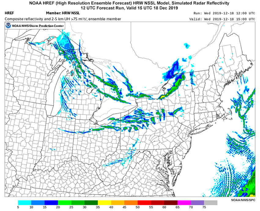
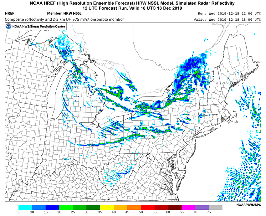
The sliders below contain simulated radar reflectivity images from the 12 UTC run of two HREF models, the HRW NSSL and the NAM Nest, valid for 15 and 18 UTC (11:00 and 14:00 EST, three and six hour forecasts).
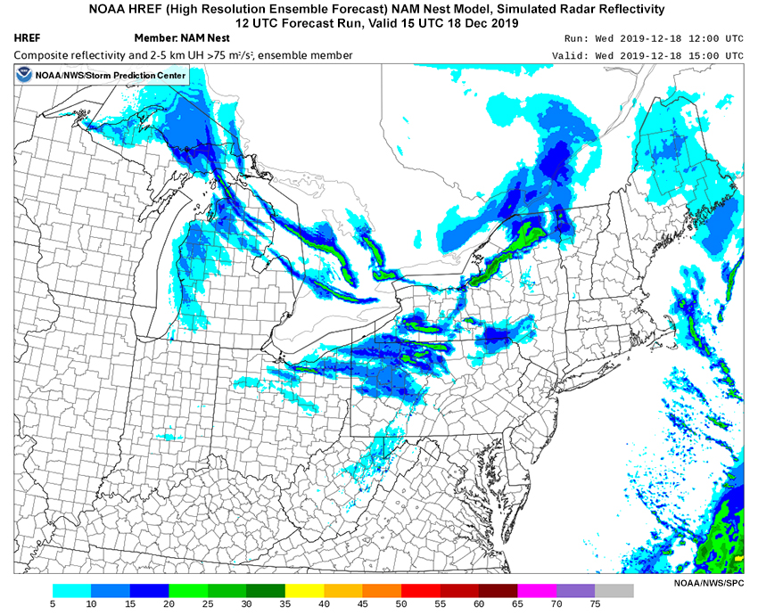
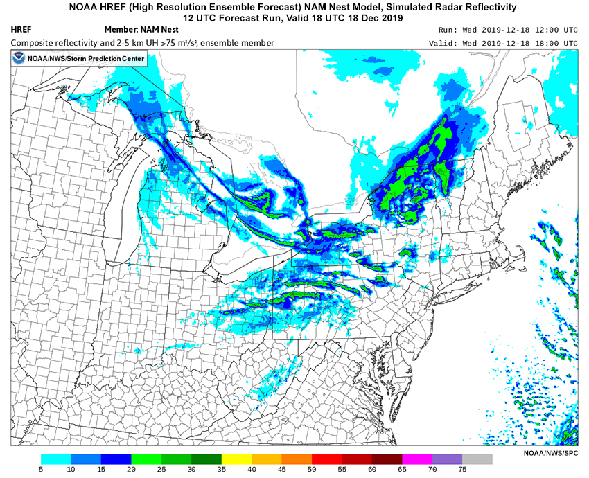
Question
What does the guidance from these models indicate as the day progresses?
The correct answers are a, b, c.
Both HREF models indicate a combination of developing convective cells and organized lines consisting of bands of snow showers and possible snow squalls. The activity continues to develop and move downstream in response to additional heating and availability of low-level moisture and instability.
The simulated composite reflectivity guidance also shows that reflectivities are mostly less than 35 dBZ, indicating low convective cloud-tops and potential overshooting by radar. These features in the simulated radar output align with a number of the features illustrated in the QLCS conceptual snow squall model, reinforcing the potential for squall activity.
Question
What would your next step be after viewing the model guidance?
Generally, after reviewing model guidance, the next step is to investigate the observations and other products available to help build confidence in the information from the models. In the next section we’ll review the data that existed when the snow squall parameter output from the RAP13 model became available.
2.0 Synoptic Analysis - 12z Model Guidance » 2.1 Further Analysis 09 to 12z Products
To validate whether the models are providing reliable guidance for the day, review the following products and answer the questions that follow.
Answer the two questions below. Use the arrows to navigate between them.
2.0 Synoptic Analysis - 12z Model Guidance » 2.2 Synoptic Analysis - Incorporating ALPW
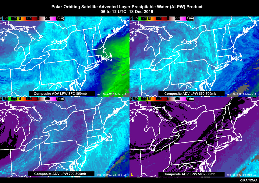
The polar-orbiting satellite-based Advected Layer Precipitable Water (ALPW) product can help inform snow squall forecasts.
Let’s take a look at what this product showed from 06 to 12 UTC on 18 December. Review the product loop, then answer the questions that follow.
Question
Why would this product be useful when forecasting the development of squalls? (Choose all that apply.)
The correct answers are a, c, d.
The satellite-based ALPW (Advected Layer PW) product is derived from microwave observations obtained from several polar-orbiting satellites. Observations are collected during the 10 hours before a common reference time/hour, advected forward in time to the reference time using GFS forecast winds, and then averaged to form one 4-layer PW product. The four layers include surface to 850 hPa, 850 to 700 hPa, 700 to 500 hPa, and 500 to 300 hPa.
As an observation/analysis tool, ALPW can be used to help corroborate both model and other observational data for a variety of synoptic weather features and precipitation applications. The emphasis in this lesson is on improving the depiction of environments conducive to snow squall formation.
Now answer the following question.
Question
What features in the ALPW product help validate what you saw in the model guidance and observations? (Choose all that apply.)
The correct answers are b, d.
The correct responses are indicated above. The ALPW shows a surface to 700 hPa moisture axis ahead of the Arctic cold front and trough aloft and indicates an enhanced potential for convection.
The availability of low-level (below ~850 hPa) moisture is another important snow squall ingredient indicated by the conceptual model. Any enhanced low-level moisture will increase the instability and therefore increase the likelihood for robust convection.
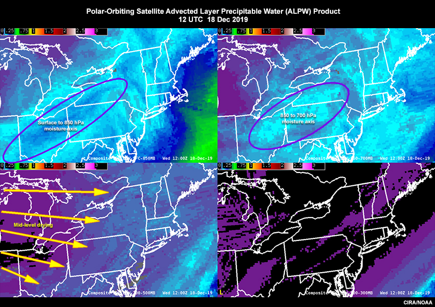
At 12 UTC, we see a southwest-to-northeast-oriented band of low-level moisture that extends from the surface to 700 hPa (upper two panels). Above that layer, the ALPW product shows drying as it advances eastward above the axis of low-level moisture. The drying is also associated with warming (as seen in water vapor imagery and in the soundings), that will act as a cap, resulting in the low-top convection—another key aspect noted in the conceptual model.
During the warm season, enhanced elevated mixed layers (EML), well known for their role in promoting high-end severe weather episodes, can often be observed in real time by following the axis of 700-500 hPa drying in ALPW images, as well as in the GOES-East band 10 lower to mid-level water vapor imagery. One potential additional advantage of the ALPW imagery is better vertically pinpointing the location of the EML (two distinct vertical layers between 500 and 850 hPa, versus one broader weighting function layer seen with the GOES-R band 10 imagery). For more information on this topic, see the article by Gitro et al. 2019, A Demonstration of Modern Geostationary and Polar-Orbiting Satellite Products for the Identification and Tracking of Elevated Mixed Layers.
Following the ALPW product into the day, we’re able to monitor the eastward movement of the low-level moisture. There are implications that convection will continue ahead of the Arctic cold front and upper-level trough.
3.0 Event Evolution from 14 to 17 UTC
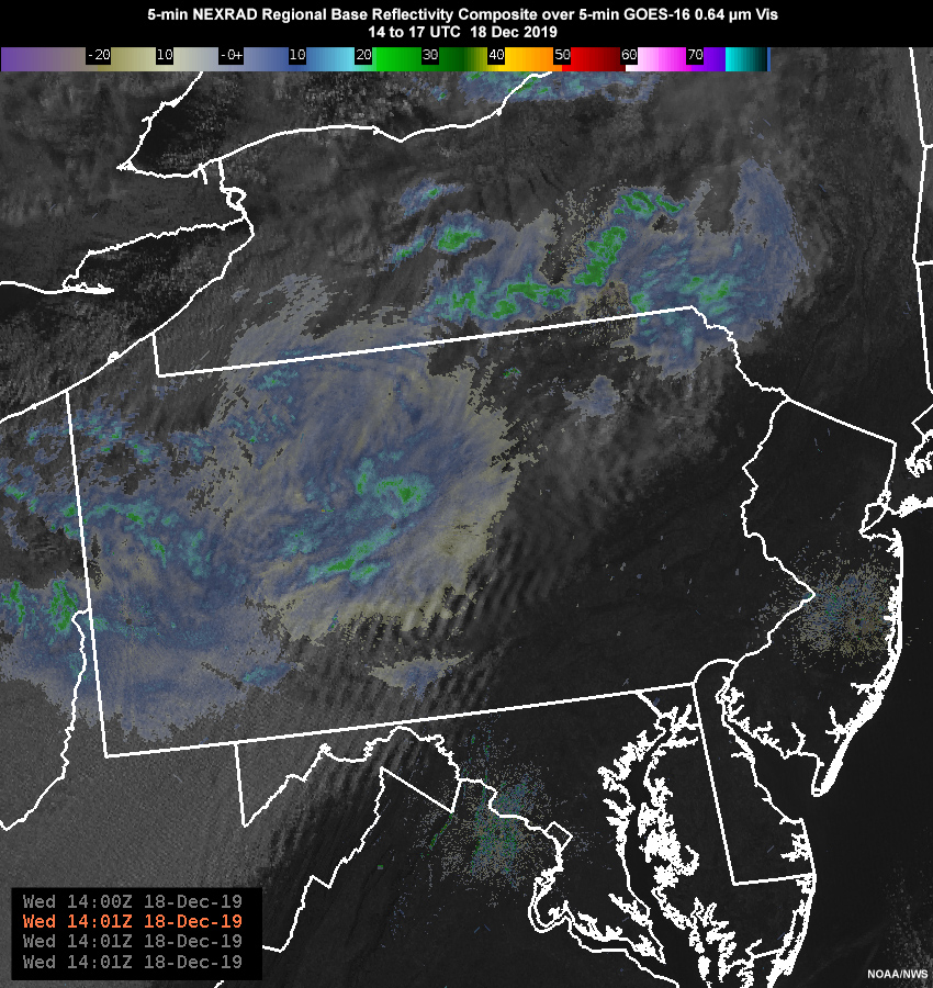
As the models and observations have indicated, the 18 December squalls continued to develop as they moved eastward. Let’s move ahead to the period from 14 to 17 UTC (9:00 to noon local time EST) to perform some more focused analysis on the development of convection during that time, using a combination of radar and satellite products.
Question
What features limit the radar observations for this event? (Choose all that apply.)
The correct answers are b, c, e.
Radar has set elevation scans; the farther you are from the radar site the greater the potential to overshoot low cloud tops. Radar coverage, especially at low-elevation scan angles, can be limited by terrain blockage. Radar sites spacing may also result in coverage gaps, again especially at low-elevation scans.
Radar is capable of diagnosing the intensity of precipitation and precipitation type, along with trends in developing convective cell and band structures. However, during events like this one, it is beneficial to have other tools at your disposal to help identify and fill in potentially missing squall features.
Answer the following question.
3.0 Event Evolution from 14 to 17 UTC » 3.1 Satellite Products Better Suited for Cloud Analysis
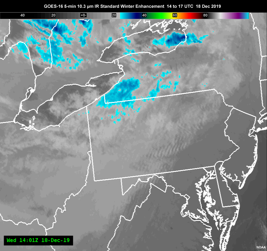
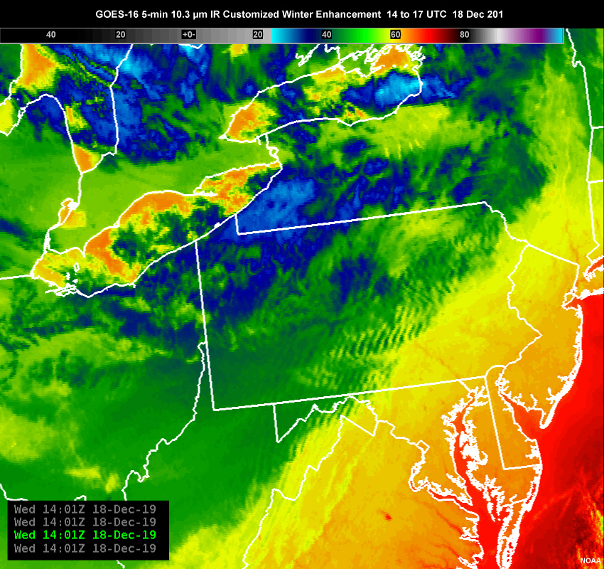
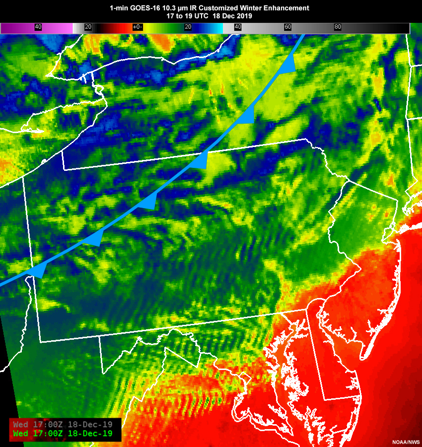
Viewing low-level cloud tops using a ‘standardized’ enhancement can be challenging. Applying a customized enhancement to 10.3 µm IR imagery can be very useful when trying to isolate cloud-top features of interest associated with events like the 18 December snow squalls.
GOES-16 5-min 10.3 µm IR Standard Winter Enhancement
GOES-16 5-min 10.3 µm IR Customized Winter Enhancement
Question
What are the benefits of viewing IR imagery with a locally customized color enhancement? (Choose all that apply.)
The correct answers are b and c.
Standardized IR enhancements are commonly created and tuned for highlighting higher/colder cloud tops associated with deeper warm-season convection. This means that colors are typically reserved for features colder than minus 30 deg C, leaving shades of grey for warmer temperatures. The warmer lower cloud tops associated with snow squalls are often warmer than minus 30 deg C and therefore appear in the range of the enhancement’s grey shades. And since humans are only capable of seeing less than 100 shades between black and white, compared to millions of unique colors, gradients in temperature stand out far less when applying a grey-scale enhancement.
The locally customized enhancement color curve shown here was developed by the State College NWS office. It is tuned for lower/warmer more shallow cloud tops that are more prevalent in wintertime convection. Modifying standardized enhancements allows forecasters to more easily identify cloud tops associated with more robust convection.
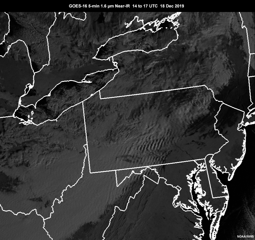
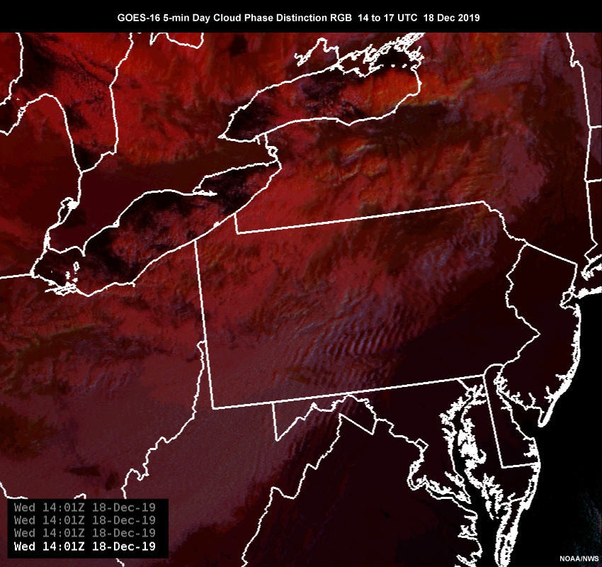
The 10.3 µm IR alone does not discriminate between liquid and ice phases within the cloud top. This additional information would be helpful in assessing precipitation intensity. Let’s take a look at the Day Cloud Phase Distinction product.
Question
What additional information does the Day Cloud Phase Distinction RGB product show? (Choose all that apply.)
The correct answers are c, d, e.
Combining the different spectral capabilities of the three bands—visible, 1.6 NIR, and 10.3 IR—gives us a high-resolution product that uses color to better contrast and discriminate between cloud and surface features (e.g. liquid water vs. glaciating cloud tops, snow-covered ground, bare ground, and water surfaces). The Day Cloud Phase Distinction RGB product is more effective in a case like this than any of its components alone.
3.0 Event Evolution from 14 to 17 UTC » 3.1 Satellite Products Better Suited for Cloud Analysis » 3.1.1 Identifying Glaciation
Question
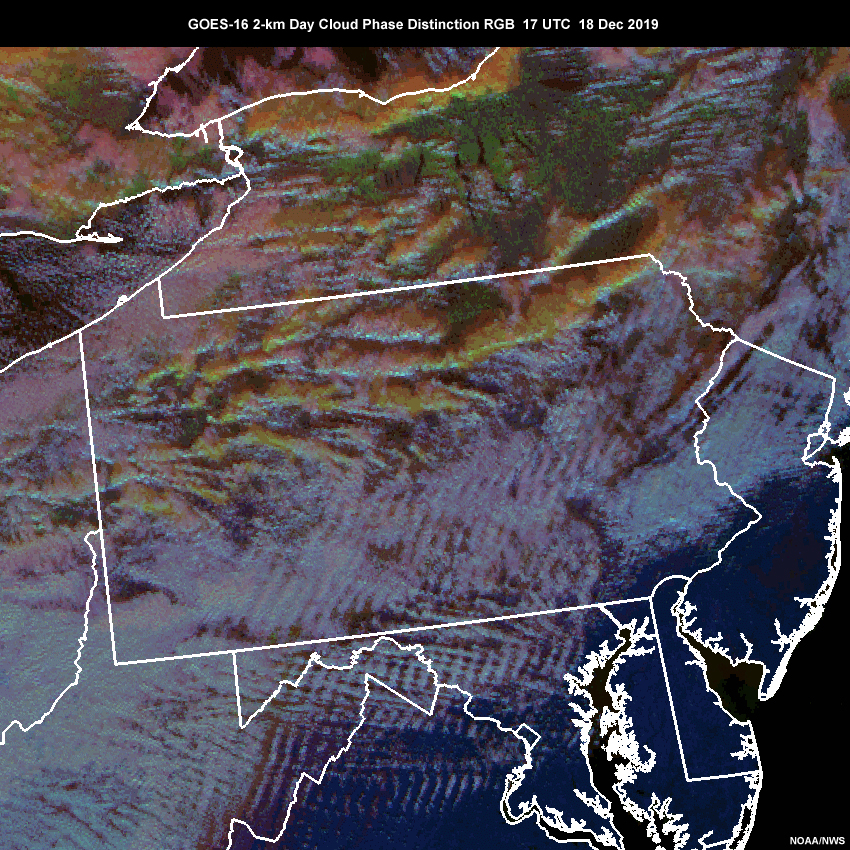
Using the magenta pen tool, circle the cloud bands that are glaciating and potentially generating snowfall.
The more robust convective cells can be identified where cyan shades transition to green, yellow and orange shading, indicating cloud top glaciation. Green indicates initial glaciation, yellow cloud tops indicated thicker ice clouds, and orange shading indicates higher-level cirrus.
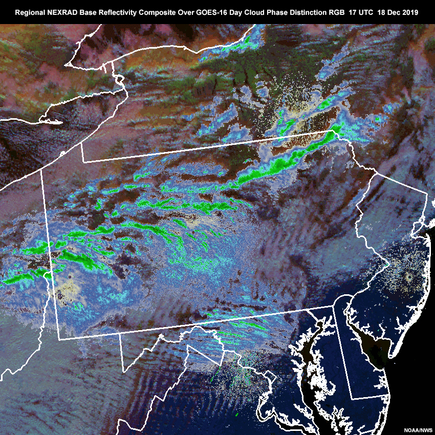
Overlaying radar reflectivity data shows how well the convective cells and bands line up with the deeper convection seen in the RGB (indicated in shades of light-green to yellow where glaciation has occurred). Snow cover in western Ohio and northern New York appears in shades of green. And low clouds dominated by water droplets are shown in shades of cyan and magenta.
For additional interpretation and background information on the Day Cloud Phase Distinction RGB, see Day Cloud Phase Distinction Quick Guide.
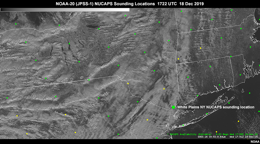
3.0 Event Evolution from 14 to 17 UTC » 3.1 Satellite Products Better Suited for Cloud Analysis » 3.1.2 17 UTC NUCAPS Sounding
NOAA Unique Combined Atmospheric Processing System (NUCAPS) soundings can also help when monitoring potential convective conditions like this. NUCAPS soundings are derived from sounders aboard the Joint Polar Satellite System (JPSS), S-NPP and European Metop satellites. For NWS users, NUCAPS soundings are currently available from the NOAA-20 (JPSS-1) satellite.
Question
Why would it be beneficial to have additional sounding data?
NUCAPS soundings provide information that can help partially fill the gaps in space and time. Conventional soundings come twice a day, at 00 and 12 UTC. NUCAPS sounding products come between 1 to 3 a.m. and p.m. local time. The mid-afternoon pass is often critical for assessing the potential for afternoon convective activity.
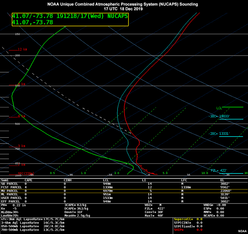
Let’s take a look at a 17 UTC NUCAPS sounding located near White Plains, New York.
Question
What does this sounding imply for the forecast?
The correct answer is a.
We can see that the NUCAPS sounding reinforces the view of instability in the boundary layer (sfc to 850 hPa) ahead of the advancing snow squalls and Arctic cold front, which will help fuel continued convective activity into the afternoon as the front approaches the eastern seaboard.
Based on model guidance, we anticipate snow shower and squall activity to affect southern Massachusetts, southeastern New York, and Long Island in the 20 to 23 UTC (3 to 6 p.m. EST) time frame.
Snow squall warnings were issued for the region between 20 and 22 UTC (3 to 5 p.m. local time EST).
Access to NUCAPS data can be viewed via the NWS AWIPS display system, or using NOAA’s Office of Satellite and Product Operations (OSPO) interactive NUCAPS Skew-T global viewer, https://www.ospo.noaa.gov/Products/atmosphere/soundings/nucaps/.
3.0 Event Evolution from 14 to 17 UTC » 3.2 17 to 19 UTC: Rapid Scan Imagery
Let’s shift our focus to the time period from 17 to 19 UTC (noon to 2 p.m. local time). As noted earlier, there were some significant impacts across central Pennsylvania as the squall activity moved eastward, including a major traffic pile-up along Interstate 80 at 1840 UTC (1:40 p.m. EST).
Take a look at the following radar and satellite products, then answer the questions that follow.
5-min Regional Base Reflectivity Composite over Standard 10.3 µm IR
1-min 10.3 µm IR Modified Enhancement
1-min Day Cloud Phase Distinction RGB
Answer the three questions below. Use the arrows to navigate between them.
3.0 Event Evolution from 14 to 17 UTC » 3.2 17 to 19 UTC: Rapid Scan Imagery » 3.2.1 Benefits of Using Satellite and Radar in Tandem
We can leverage the respective strengths of radar and satellite imagery to create and refine a more complete analysis of convective activity across the region.
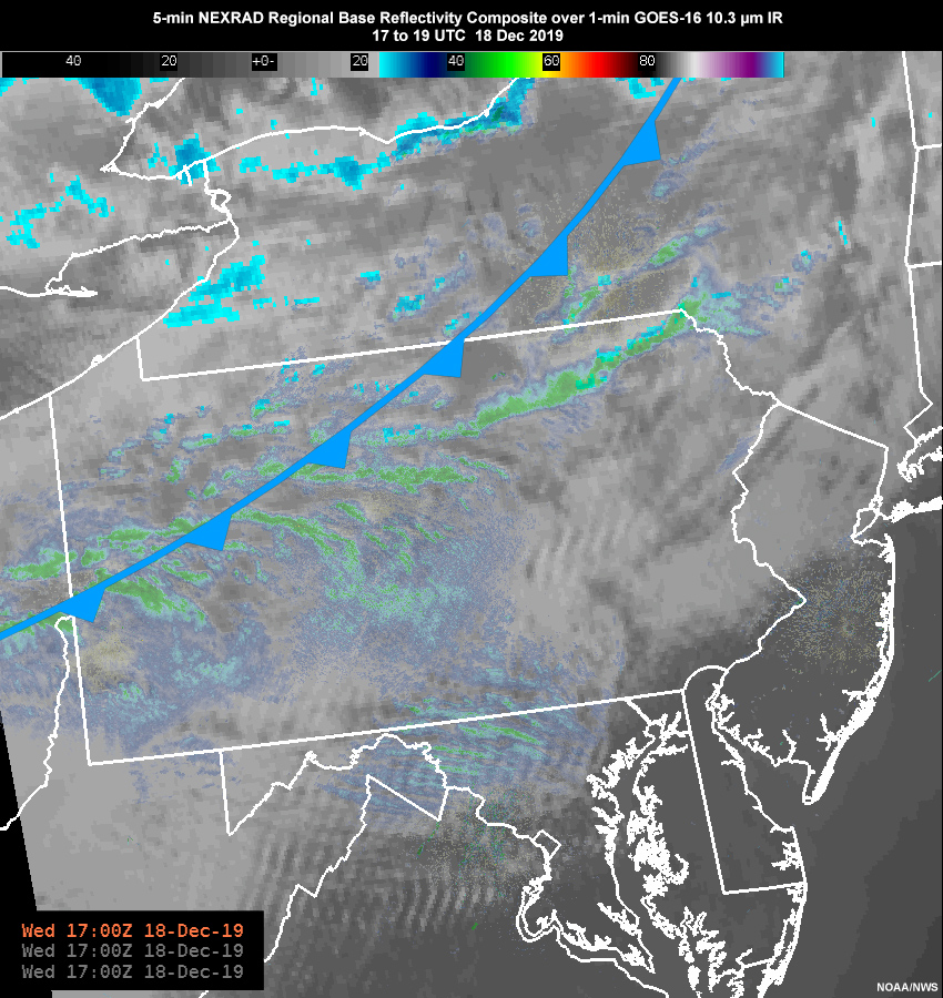
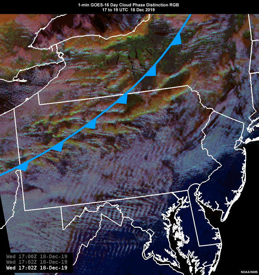
5-min Regional NEXRAD Base Reflectivity Composite over 1-min GOES-16 10.3 µm IR
5-min NEXRAD Regional Base Reflectivity Composite over 1-min GOES-16 Day Cloud Phase Distinction RGB
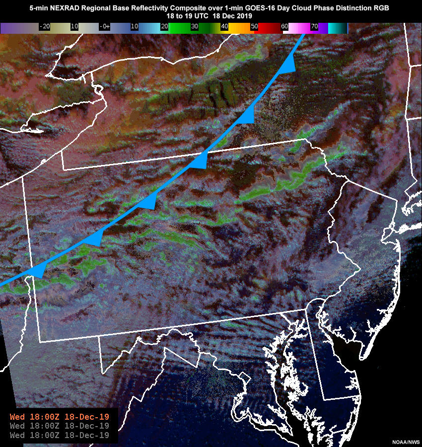
While radar provides reliable quantitative information on cell intensity, satellite can help us extrapolate from the radar view to extend spatial coverage into areas where radar coverage may be weaker or missing (due to either overshooting, beam blockage, or range limit issues).
We can see that the radar composite captures most of the convective activity. View the loops from 18 to 19 UTC in the tabs below, then answer the question that follows.
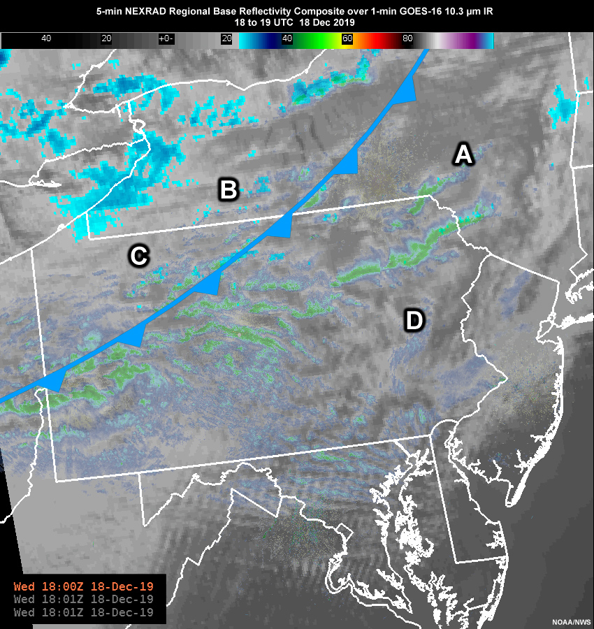
5-min Regional NEXRAD Base Reflectivity Composite over 1-min GOES-16 10.3 µm IR
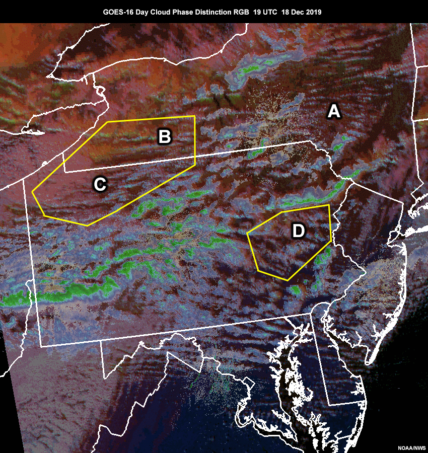
1-min GOES-16 Day Cloud Phase Distinction RGB

Question
Which location(s) may contain gaps in the radar coverage? (Choose all that apply.)
The correct answers are b, c, d.
B, C and D are the correct responses. There are some identifiable weaknesses in the coverage, or gaps, such as over far-northern and northwestern Pennsylvania and across the border into southwestern New York, where the reflectivity values are either underestimated or possibly missed altogether. Another area of concern appears in east-central Pennsylvania, where glaciating cloud tops in the RGB indicate deeper convection but radar reflectivities are either weak or missing.
This could be due to either range limitations, areas where the lowest-elevation scans overshoot the shallow convection, or beam blockage at the lowest-elevation scans.
4.0 Impacts and Takeaways
The 18 December snow squalls in central Pennsylvania contained a dangerous mix of conditions that led to multiple hazards for travelers. In this case, the combination of slick roads and low visibility proved fatal.
It is imperative that forecasters employ the most effective tools at their disposal to provide useful and actionable information for air and ground-transportation customers impacted by rapidly changing winter weather. By effectively incorporating satellite products into their forecasting processes in tandem with radar, model output, and traditional soundings, forecasters are better equipped to diagnose, monitor, and communicate about this type of hazardous event.
Key Takeaways
Question
Identify the most significant application of each satellite product below for forecasting and monitoring snow squalls.
The information provided by these satellite products offers multiple benefits::
- Near-IR imagery can help characterize cloud-top phase and therefore detect glaciation as convection grows.
- Locally modified IR enhancement curves can help isolate the shallow low-top convective cloud temperature ranges characteristic of snow squall events.
- Customized color enhancement of radar products can help forecasters identify the less intense reflectivities associated with snow squall activity.
- The Day Cloud Phase Distinction RGB product combines the strengths of visible (cloud texture), 1.6 µm near-IR (cloud phase), and 10.3 µm longwave IR (cloud top temperature) imagery into a single product that uses color to qualitatively characterize cloud-top microphysical properties (e.g. cloud phase) and surface features.
- Rapid-scan imaging provides more frequent updates (e.g. compared to radar) for identifying and monitoring rapid development and trends in convection.
- JPSS derived soundings (e.g. NUCAPS soundings) provide snapshots of the thermodynamic environment in between conventional sounding times (00 and 12 UTC), providing additional information on the availability of low-level instability, important for snow squall formation and maintenance.
- The near real-time polar-orbiting microwave-based ALPW product provides hourly updates on the vertical distribution of layered precipitable water, contributing to situational awareness on low-level moisture availability important for shower and squall development and maintenance.
Generally speaking, GEO (e.g. GOES-R) and LEO (e.g. JPSS) satellites have imaging and sounding capabilities that offer complementary observations for diagnosing the potential for snow squall activity and for assisting with nowcasting of snow squall events. The higher spatial and temporal resolution provided by satellite observations can assist with detection of often subtle environmental and convective signatures associated with snow squall formation and propagation.
Here are a few other key takeaways:
- The GOES-R imagery toolbox for analyzing the snow squall environment includes the three water-vapor bands, visible and near-IR bands, longwave IR, and derived RGB products (e.g. Day Cloud Phase Distinction RGB).
- Water-vapor imagery can help validate the synoptic and mesoscale features and ingredients important for snow squall development.
- Visible imagery provides a high-resolution view of developing convection.
- RGB imagery such as the Day Cloud Phase Distinction RGB product presented in this lesson, uses color to characterize cloud top phase and help assess cloud top glaciation for developing convection.
Through the use of specific and more finely tuned satellite products in combination with model guidance, radar, soundings, and other conventional observations, you should be better equipped to diagnose the potential snow squall environment, identify the snow-producing cells, and forecast their evolution.
5.0 Resources and References
Resources
The following resources provide additional online information on satellite data and topics presented in this lesson:
NOAA Virtual Lab: Satellite Training and Operations Resources (STOR)
https://vlab.ncep.noaa.gov/web/stor
CIRA/RAMMB/VISIT Quick Information Guide: Advected Layer Precipitable Water (ALPW) product
http://rammb.cira.colostate.edu/training/visit/quick_guides/
CIRA/RAMMB ALPW Realtime Product Webpage
http://cat.cira.colostate.edu/sport/layered/advected/LPW_alt.htm
References
The following publications provide additional information on the topics presented in this lesson.
Banacos, P.C., G.A. DeVoir, B. Watson, A.N. Loconto, and D.J. Nicosia, 2019: R2O: Development of NWS Snow Squall Warnings. Preprints, 9th Conference on the Transition of Research to Operations, Amer. Meteor. Soc., Phoenix, AZ, 6-10 Jan 2019. [Available online from https://ams.confex.com/ams/2019Annual/meetingapp.cgi/Paper/349919]
Bryan, G.H., and J.M. Fritsch, 2000: Moist absolute instability: The sixth static stability state. Bull. Amer. Meteor. Soc., 81, 1207-1230. [Available online from https://doi.org/10.1175/1520-0477(2000)081%3C1287:MAITSS%3E2.3.CO;2]
Devoir, G.A., 2004: High Impact Sub-Advisory Snow Events: The Need to Effectively Communicate the Threat of Short Duration High Intensity Snowfall. Preprints, 20th Conference on Weather Analysis and Forecasting/16th Conference on Numerical Weather Prediction, Amer. Meteor. Soc., Seattle, WA, 12-16 Jan 2004. [Available online from https://ams.confex.com/ams/84Annual/techprogram/paper_68261.htm]
Forsythe, J.M., S.Q. Kidder, K.K. Fuell, A. LeRoy, G.J. Jedlovec, and A.S. Jones, 2015: A multisensor, blended, layered water vapor product for weather analysis and forecasting. J. Operational Meteor., 3 (5), 41–58. doi: http://dx.doi.org/10.15191/nwajom.2015.0305
Gitro, C.M., Bikos, D., Szoke, E.J., Jurewicz Sr., M.L., Cohen, A.E., and M.W. Foster, 2019. A demonstration of modern geostationary and polar-orbiting products for the identification and tracking of elevated mixed layers. J. Operational Meteor., 7 (13), 180-192. doi: https://doi.org/10.15191/nwajom.2019.0713.
Contributors
COMET Sponsors
MetEd and the COMET® Program are a part of the University Corporation for Atmospheric Research's (UCAR's) Community Programs (UCP) and are sponsored by
- NOAA's National Weather Service
(NWS)
with additional funding by: - Bureau of Meteorology of Australia (BoM)
- Bureau of Reclamation, United States Department of the Interior
- European Organisation for the Exploitation of Meteorological Satellites (EUMETSAT)
- Meteorological Service of Canada (MSC)
- NOAA National Environmental Satellite, Data and Information Service (NESDIS)
- NOAA's National Geodetic Survey (NGS)
- National Science Foundation (NSF)
- Naval Meteorology and Oceanography Command (NMOC)
- U.S. Army Corps of Engineers (USACE)
To learn more about us, please visit the COMET website.
Project Contributors
Project Leads
- Patrick Dills - UCAR/COMET
- Tony Mancus - UCAR/COMET
Instructional Design
- Tony Mancus - UCAR/COMET
Science Advisors
- Patrick Ayd - NWS Weather Forecast Office, Duluth, MN
- Dan Baumgardt - NWS Weather Forecast Office, LaCrosse, WI
- Greg DeVoir - NWS Weather Forecast Office, State College, PA
- Patrick Dills - UCAR/COMET
- Michael Jurewicz - NWS Weather Forecast Office, State College, PA
- David Radell - NWS Weather Forecast Office, New York, NY
- Chauncy Schultz - NWS Weather Forecast Office, Bismarck, ND
- Phil Schumacher - NWS Weather Forecast Office, Sioux Falls, SD
Program Oversight
- Amy Stevermer - UCAR/COMET
Graphics/Animations
- Steve Deyo - UCAR/COMET
- Patrick Dills - UCAR/COMET
Multimedia Authoring/Interface Design
- Gary Pacheco - UCAR/COMET
COMET Staff, September 2020
Director's Office
- Dr. Elizabeth Mulvihill Page, Director
- Tim Alberta, Assistant Director Operations and IT
- Dr. Paul Kucera, Assistant Director International Programs
- Dr. Wendy Gram, Implementation Manager
Business Administration
- Lorrie Alberta, Administrator
- Auliya McCauley-Hartner, Administrative Assistant
- Tara Torres, Program Coordinator
IT Services
- Bob Bubon, Systems Administrator
- Joey Rener, Software Engineer
- Malte Winkler, Software Engineer
Instructional Services
- Dr. Alan Bol, Instructional Designer/Scientist
- Tony Mancus, Instructional Designer
- Sarah Ross-Lazarov, Instructional Designer
- Tsvetomir Ross-Lazarov, Instructional Designer
International Programs
- David Russi, Translations Coordinator
- Martin Steinson, Project Manager
Production and Media Services
- Steve Deyo, Graphic and 3D Designer
- Dolores Kiessling, Software Engineer
- Gary Pacheco, Web Designer and Developer
- Tyler Winstead, Web Developer
Science Group
- Patrick Dills, Meteorologist
- Bryan Guarente, Instructional Designer/Meteorologist
- Adam Hirsch, Meteorologist
- Matthew Kelsch, Hydrometeorologist
- Brianna Lund, Meteorologist
- Andrea Smith, Meteorologist
- Amy Stevermer, Scientist/Instructional Designer
- Vanessa Vincente, Meteorologist