Welcome
After completing this module, you should be able to do the following things:
- List the properties that ocean models forecast
- Recall the size of features that mesoscale ocean models can forecast
- Describe the assumptions that go into an ocean model
- List the limitations to ocean model forecasts
- Identify the following ocean structures in forecast products:
- Current systems
- Fronts
- Eddies
- Identify the following ocean phenomena in forecast products:
- Eddy formation and dissipation
- Upwelling
- Internal tides
- Describe operational applications of ocean models
- Recall the major defining attributes of the following operational ocean models:
- Navy Layered Ocean Model (NLOM)
- Navy Coastal Ocean Model (NCOM)
- Hybrid Coordinate Ocean Model (HYCOM)
- Shallow Water Analysis and Forecast System (SWAFS)
- Advanced Circulation Model (ADCIRC)
We recommend that you complete the module Introduction to Ocean Models (http://meted.ucar.edu/oceans/ocean_models), before you start this one.
Introduction
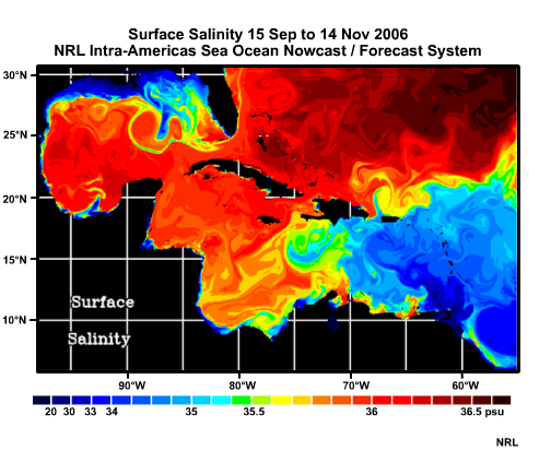
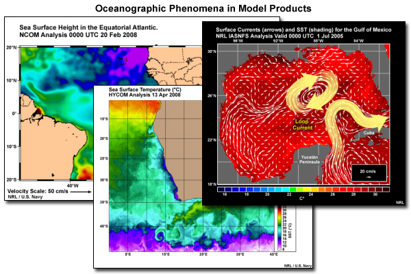
Mesoscale ocean circulation models simulate the properties of seawater as it moves and evolves through the ocean basins. These models have sufficient resolution to analyze and forecast processes like eddy formation and dissipation. We refer to these processes as mesoscale processes and define them as having horizontal dimensions on the order of at least one degree of latitude (about 100 km), like those shown in this example.
In the module Introduction to Ocean Models, we looked at the elements used to build an ocean model. Now we will look at some of the information they provide.
In this module we will treat the computational structure of ocean models primarily as a “black box”. We will focus instead on the result of ocean models and not on how they actually work (i.e., their physics and numerics).
Introduction » Ocean Properties that Models Simulate
Mesoscale ocean circulation models simulate several ocean properties:
- Temperature. From the surface to the seafloor. Temperature is the major factor in determining seawater properties such as density and sound speed.
- Salinity. Just as the atmosphere has humidity or water vapor as its major contaminant, the ocean has salinity. Ocean models need to simulate salinity (or conversely, fresh water content) because it is one factor in the determination of density, along with temperature and pressure.
- Currents. The horizontal and vertical movement of seawater profoundly affects the temperature and salinity in the ocean. Gradients across currents result in complex structures, such as fronts and eddies. Vertical motions like upwelling can radically alter ocean temperatures over very short time periods. Stronger currents directly affect marine operations.
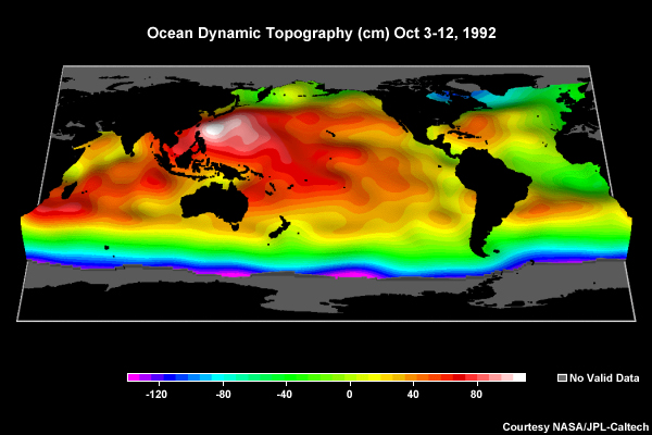
- Elevation or sea surface height (SSH). SSH is controlled by the density of the seawater along with some dynamic effects from currents. Elevation is also the consequence of tides (as well as some currents)
Introduction » Time and Space
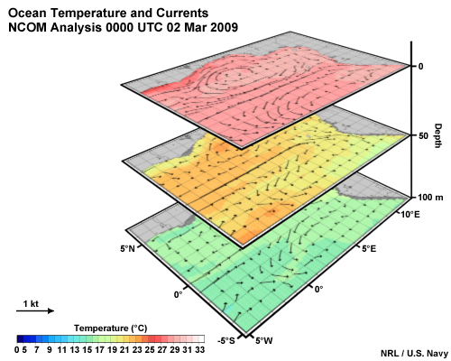
Ocean models simulate these properties in 3 dimensions through a period of time. In operational models, this time may start with a reanalysis of the past (a hindcast) or an analysis of current conditions (a nowcast), and continue out into the future (a forecast). Operationally, the Naval Oceanographic Office (NAVO) and NOAA’s National Center for Environmental Prediction (NCEP) produce hindcasts at 3-hour steps from 120 to 24 hours before the analysis time and forecasts from the analysis time out to as much as 120 hours after the analysis. Results are saved at 1-, 3-, or 6-hr steps. This graphic shows surface currents and temperatures around the Gulf Stream at 3-hour intervals as forecast by the Navy Coastal Ocean Model (NCOM).
Introduction » Model Output
Model output is usually delivered to forecasters as graphic forecast products. Additionally, NOAA and the U.S. Navy make data files available via various servers.
Most model forecast products take the form of maps. Since most marine operations take place on the surface, maps work well for most applications. Many other applications, however, require information about ocean properties in three dimensions, such as sound speed or subsurface currents. For these applications, data fields may be made available or maps for a given depth or cross sections can be constructed from these files.
Model Limitations
Models make several assumptions in order to simplify computations, deal with processes that can’t be modeled, and run efficiently, as discussed in the previous module. The resulting efficiency allows the completion of a model run in time to be useful. Thus, all computer models have limitations. Here we describe several of the limitations that are faced when modeling the ocean.
Model Limitations » Numerics
Models are inherently limited because they are trying to describe an analog or continuous environment digitally. That is, they are computing the movement of information through a discreet spatial grid at discreet time steps. And no matter how many decimal places or bits are used, there will be rounding and truncation errors during computations. These errors can be managed, but not completely, so a model that involves lots of calculations can “drift” away from reality.
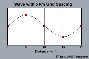
Errors from spatial aliasing will result for features that are less than 5 grid points in size. Thus a model running with a grid spacing of 1/12° (9 km/5 nm) can only accurately depict features that are greater than 20 nm in size. Similarly, a higher resolution 1/24° (4.6 km/2.5 nm) model can accurately depict smaller features greater than 10 nm in size. What does this mean? A mesoscale model needs to properly depict fronts and eddies that are important to model users.
Another numerical limitation comes from parameterization. Because the processes forcing the ocean model mostly occur on a sub-grid scale, they are described by some sort of simplifying mathematical relationship or parameterized. All parameterizations represent approximations and hence have limitations.
There are always computational tradeoffs. It may some day be possible to run global ocean models from pole to pole at 100m horizontal resolution with 500 layers, but the computational power (or storage) to do this and get products out in a timely manner isn’t yet available. Modelers have to make choices between what they would like to do and what they can.
Model Limitations » Post-Processing
When a model run is complete, no storage system could hold all the information it is capable of producing, so only selected data fields are saved. For example, from the 50 or more vertical levels in a model only a handful are plotted as forecast products and those only at selected time intervals (usually 3, 12, or 24 hours). For processes that operate on shorter timescales, like tides, this can make it hard to present a precise forecast.
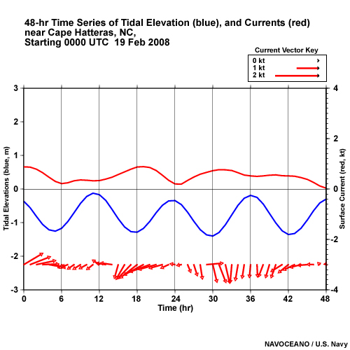
For processes that operate on very short time scales, your best solution may be a time series plot for a selected location. This graphic shows a time series of water elevation and surface currents for a location near Cape Hatteras, NC.
Model Limitations » Observations - Quantity
Through a process called assimilation, data from observations are used to bring models closer to the true state of the ocean. These observations come from satellites, ships, gliders, and fixed or drifting buoys. However the ocean data we use suffer from both sparseness and possible inaccuracies.
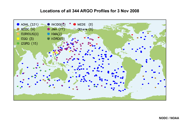
For example, we gather about 500 temperature and salinity vertical profiles per day across all of the world’s oceans. These observations provide the majority of our subsurface data.
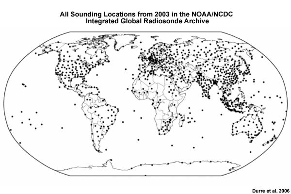
By comparison, atmospheric models assimilate over 3000 atmospheric soundings per day (two atmospheric soundings per day from over 1500 locations). This is even a greater discrepancy between ocean and atmospheric models when one considers that 70% of the Earth’s surface is covered by water.
Model Limitations » Observations - Quality
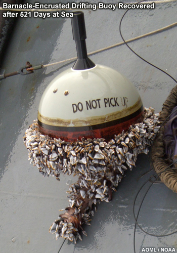
In addition to the small quantity of observations, the quality of ocean observations varies tremendously. The ocean is not kind to instruments. For example, this picture shows a drifting buoy covered with barnacles. It was recovered after 521 days at sea. Such biofouling degrades instrument performance. Instruments also suffer sensor drift, and other troubles. And, unlike the local weather station, when an ocean sensor goes bad, a repairman just can’t walk out and fix it.
Model Limitations » Model Forcing
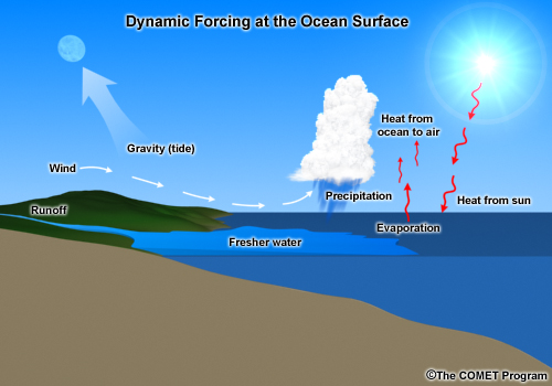
Additional ocean model limitations may arise from the atmospheric forcing that drives the ocean. All major changes to ocean properties occur at the surface. Anything that happens at depth will be the result of mixing or diffusion processes. This forcing at the air-sea interface includes momentum from wind stress, heat fluxes at various wavelengths, pressure, and mass (water) exchanges due to evaporation, precipitation, and river runoff. Nearly all of this information comes from numerical weather prediction (NWP) models. Ocean models use this information to transfer heat in and out of the mixed layer and to generate currents.
As we are well aware, the weather models are not perfect. For a host of their own reasons, they sometimes miss the mark. Air-sea interchange processes are particularly hard to model. Thus, errors in weather models that force ocean processes will result in errors in ocean models.
Model Limitations » Assimilation Routines
The assimilation of observations into the analysis or “start field” before a model forecast run can also lead to problems. First off, let’s be clear: the assimilation of observed data generally improves forecast skill. That’s why we do it, despite the fact that it is difficult and computationally expensive to do properly. As an example, these plots show the result of a validation experiment for the 1/32-° (~2 nm) NLOM in the Arabian Sea. The first image shows an analysis of SeaWIFS ocean color, the second shows a “free-running” NLOM analysis without data assimilation, and the third shows the same NLOM analysis, but with assimilation of satellite altimeter data. It is clear that the location and shape of currents and eddies are more accurately simulated by NLOM when the satellite data is assimilated.
There are several ways to assimilate data and the best methods are computationally expensive, so they are generally not used in operational models today. There is active research to overcome these issues.
Model Limitations » Model Confidence
As with weather forecasts, the ways in which we use ocean model forecasts hinge on how accurate we feel they are. For example, we know that model forecasts degrade with time. Thus we tend to avoid making decisions that depend on specific details presented in a long-range forecast. However, due to the random distribution, limited quantity, and sometimes questionable quality of observations mentioned earlier, it is difficult to validate ocean models. Doing so requires dedicated field projects to gather large quantities of high resolution data, something that doesn’t happen very often.
Model Limitations » Questions
Question 1
Mesoscale ocean circulation models simulate which of the following ocean properties? (Choose all that apply.)
The correct answers are a), c), and d).
Mesoscale ocean circulation models simulate currents, salinity, sea surface height, and temperature.
Question 2
What is the size of the smallest feature that can be depicted by a model with grid spacing of 1/24 degree (4.6 km/2.5 nm) without spatial aliasing? (Choose the best answer.)
The correct answer is b) 10 nm.
Errors from spatial aliasing will result for features that are less than 5 grid points in size. Five grid points span 4 grid spacings. Thus a model running with a grid spacing 1/24 degree (4.6 km/2.5 nm) model can accurately depict features greater than 10 nm in size.
Question 3
Why do we only save data from selected levels and times for each model run? (Choose the best answer.)
The correct answer is c).
When a model run is complete, no storage system could hold all the information it is capable of producing, so only selected data fields are saved.
Question 4
On a typical day, are there more vertical profiles taken in the ocean or the atmosphere? (Choose the best answer.)
The correct answer is a).
More in the atmosphere. We gather about 500 temperature and salinity vertical profiles per day across all of the world’s oceans. By comparison, we collect over 3000 atmospheric soundings per day (two atmospheric soundings per day from over 1500 locations).
Question 5
Data for forcing in ocean models comes primarily from? (Choose the best answer.)
The correct answer is a).
All major changes to ocean properties occur at the surface. This forcing at the air-sea interface includes momentum from wind stress, heat fluxes at various wavelengths, pressure, and mass (water) exchanges due to evaporation, precipitation, and river runoff. Nearly all of this information comes from numerical weather prediction (NWP) models.
Oceanography from Models
Mesoscale ocean models give us a three-dimensional view of currents, temperature, salinity, and surface elevation through the hindcast and forecast periods. Using these models we can see a variety of structures and processes in the ocean. This section looks at some of them.
Oceanography from Models » Oceanographic Structures
Using the information in a model simulation, we can see many different types of structures in the ocean, including currents, fronts, and eddies.
Oceanography from Models » Oceanographic Structures » Current Systems
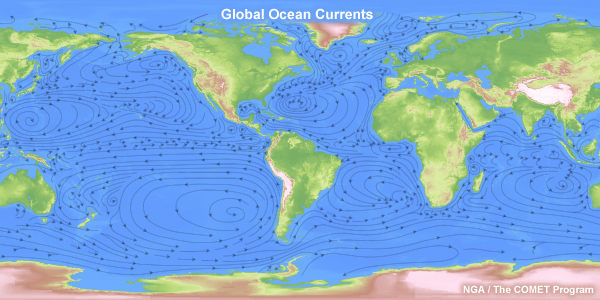
Ocean models depict current systems at all scales, so long as they span enough grid cells to be accurately depicted. For example, the ocean basin gyres appear in all models although models (which attempt to show the “real ocean”) will never look this smooth.
Oceanography from Models » Oceanographic Structures » Western Boundary Currents
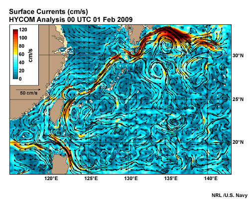
The strongest currents in the ocean tend to be western boundary currents like the Gulf Stream, Kuroshio Current, and Agulhas Current. Ocean circulation models capture these features well.
As we can see in these model nowcasts, these currents only follow relatively straight lines when they are constrained by the continental shelf along the east coast of continents. Freed from those constraints, the currents follow a sinuous path with frequent loops and meanders. Occasionally, these loops break away and form closed circulating cells or eddies that persist for long periods.
Oceanography from Models » Oceanographic Structures » Monsoon Currents
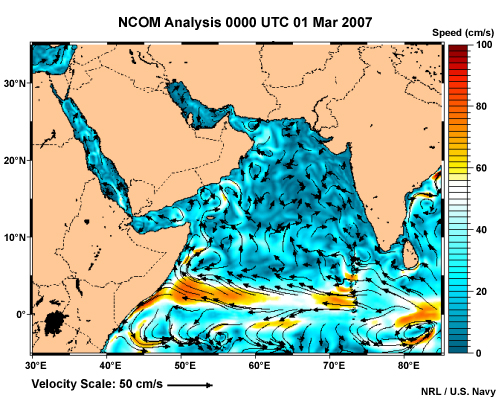
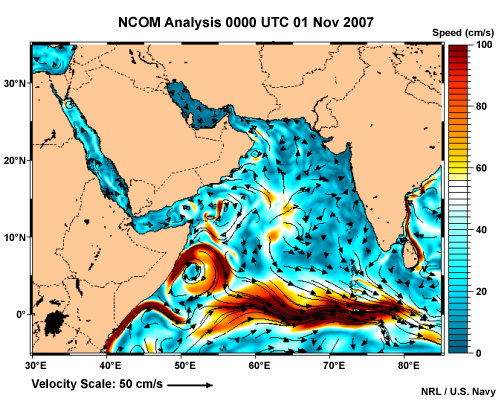
Ocean circulation models also capture seasonal variations in currents. Here we see the seasonal reversal in the equatorial current in the Arabian Sea. This event occurs every year in response to a complex ocean-atmosphere environment that includes reversing monsoon winds.
Oceanography from Models » Oceanographic Structures » Currents at Depth
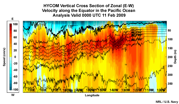
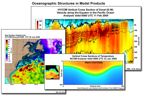
Currents at the surface may not reflect what is happening deeper in the ocean. And because satellites don’t directly detect subsurface currents that ocean circulation models predict, most of our understanding of subsurface currents comes from special observation campaigns, or models which can only occasionally be validated by observations. For example, this plot shows a cross section of current speed from west to east across the equatorial Pacific. The cool colors near the surface indicate the westward-flowing equatorial current, while the warm colors at depth indicate a much larger eastward-flowing subsurface countercurrent.
Oceanography from Models » Oceanographic Structures » Fronts-1
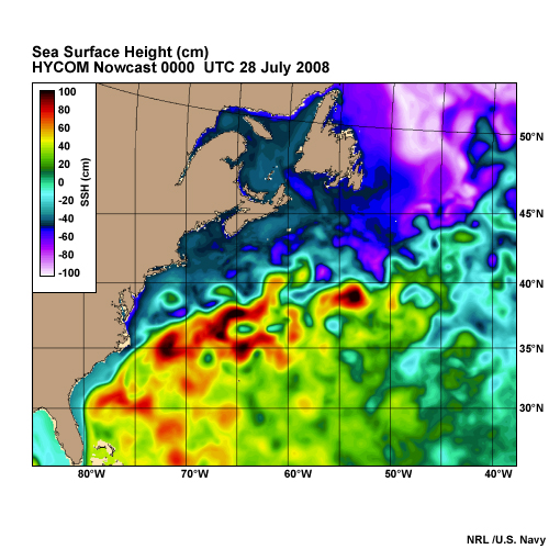
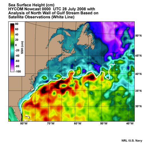
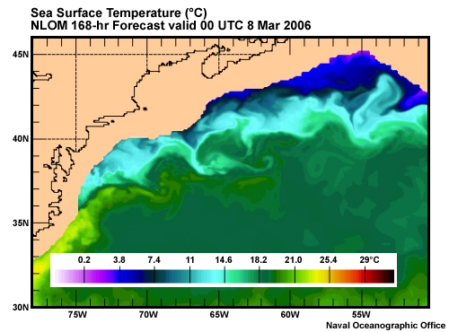
Similar to the atmosphere, ocean fronts separate water bodies with distinct characteristics. In this plot of sea surface height (SSH) in the Northwest Atlantic Ocean, the Gulf Stream North Wall Front is indicated by higher elevations in the warmer temperatures of the Gulf Stream and Sargasso Sea and lower elevations from the colder water of the Labrador Current. Strong gradients in height (horizontal changes) and temperature lie along fronts between cold (blue) and warm (red) water. The Gulf Stream, which flows northeastward to the right of this front, is a geostrophic expression of the elevation-produced pressure gradient.
Question 6
On the image below:
- Use the pen to trace out the ocean front.
When you have finished, select Done.
Compare your answer to the answer below.
Please continue watching the video above.
The white line shown here is an independent frontal analysis performed at the Naval Oceanographic Office. It is based on sea surface temperature (SST) observations rather than the modeled SSH. With that caveat, your line should follow roughly the same path. In this instance, the model does a very good job of simulating the meanders of the Gulf Stream, and thus the location of the front.
Oceanography from Models » Oceanographic Structures » Fronts-2
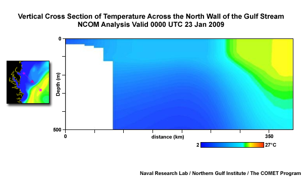
This graphic shows a cross section of temperature across the north wall of the Gulf Stream to the northeast of Cape Hatteras, NC. We can see isotherms sloping down from cold to warm water across the front. We also see that the mixed layer is nearly twice as deep in the warm water as it is in the cold water.
We look for ocean fronts in the temperature, surface height, and salinity fields. Horizontal movement or advection as the result of major current systems like the Gulf Stream or Kuroshio Current typically maintains ocean fronts. Without the introduction of warm water from equatorial regions, mixing and diffusion will eventually reduce the difference between water masses.
Oceanography from Models » Oceanographic Structures » Eddies-1
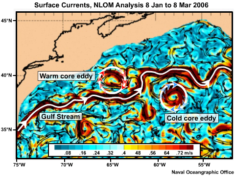
Eddies are closed circulation loops that form when tight meanders split off from a continuous current. In this example, over a two month period, we see a warm core eddy form to the north of the Gulf Stream and a cold core eddy form to the south. Once formed, these eddies migrate back toward the west.
Oceanography from Models » Oceanographic Structures » Eddies-2

Obviously, we can find eddies in model current fields. It is less obvious that mesoscale eddies, which are tens to hundreds of kilometers across, will have either a warm core or a cold core. Thus we can see them in model temperature products. Here we see surface maps and cross sections of temperature across a warm eddy in the Gulf of Mexico and a cold eddy near the Gulf Stream. Each cross section is about 500 kilometers across and 500 meters deep. In the warm core eddy, the mixed layer depth nearly doubles across the middle of the eddy, in response to converging surface flow. In the cold core eddy, the cold water rises into the center of the eddy in response to divergence at the surface, which results in upwelling. Many fishermen seek out cold core eddies because of the increased productivity spawned by the upwelling of nutrients for the food chain.
Oceanography from Models » Oceanographic Structures » Eddies-3
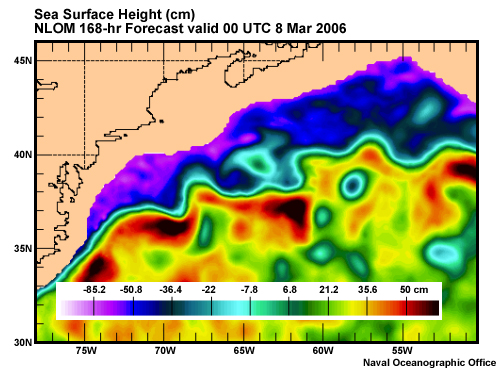
And because warmer ocean temperatures lead to higher sea surface heights and vice versa, we can frequently find eddies in SSH fields. In this example, it is much easier to find eddies in the SSH than the SST. This occurs because strong surface heating/cooling can mask the actual gradients in the SST field.
Oceanography from Models » Oceanographic Structures » Questions
Question 7
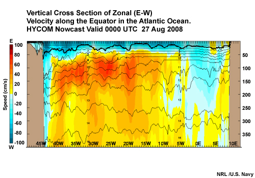
This vertical cross section shows current speed in an E-W direction (positive to the east) along the equator in the Atlantic Ocean. What oceanographic feature does this cross section show? (Choose the best answer.)
The correct answer is a) Equatorial undercurrent.
In this cross section we see both the equatorial surface current and its corresponding undercurrent. Equatorial currents at the surface flow to the west (negative velocities, shown in shades of green/blue). The equatorial undercurrent flows to the east (positive velocities, shown in shades of yellow/red).
Question 8
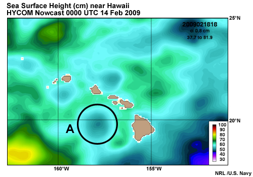
This plot shows sea surface height near Hawaii. Use the pull-down menu to choose the best answer.
The correct answers are highlighted above.
The map shows a depression in sea surface temperature. Since colder temperatures lead to lower sea surface heights, we can deduce that this is a cold core eddy. Cold core eddies exhibit cyclonic circulation, counterclockwise in the Northern Hemisphere. Another way to think of this is that water flowing into the surface depression is deflected to the right, resulting in cyclonic circulation.
Question 9
Select the correct words to complete the sentence.
The correct answers are shown above.
In a warm core eddy, the mixed layer deepens in the center, while in a cold core eddy the mixed layer shallows.
Question 10
On the image below:
- Use the pen to trace the ocean front near Japan.
When you have finished, select Done.
Compare your answer to the answer below.
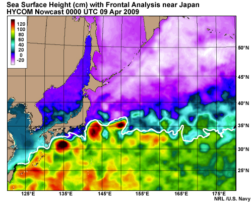
The white line shown here is an independent frontal analysis performed at the Naval Oceanographic Office. Your line should follow roughly the same path.
Oceanography from Models » Ocean Phenomena
Ocean models let us study processes such as eddy formation, movement, and dissipation, upwelling and downwelling, and internal tides. Models allow us to observe these phenomena and see how they are affected by various processes. For example, we can run multiple model versions and by carefully changing various parameters, we can attempt to determine the role of different processes.
Oceanography from Models » Ocean Phenomena » Eddy Formation and Dissipation
Eddies form in response to several different processes. We can use ocean circulation models to capture and study these processes. One type of eddy, a retroflection eddy, forms when current meanders become overextended and pinch off. Here, we see this process occurring with the Loop Current in the Gulf of Mexico.
The Loop Current is a warm ocean current in the Gulf of Mexico. It enters the Gulf from the south between Cuba and the Yucatán peninsula and exits to the east through the Florida Straits, where it becomes the Gulf Stream. The Loop Current follows a variable path. At one extreme, it flows almost directly from the Yucatan Straits along the north coast of Cuba to the Florida Straits. At the other extreme, the Loop Current flows far north before looping clockwise back to the south. The Loop Current returns to its more direct configuration by slowly pinching off its northward extension to form a large, warm-core eddy. This eddy then drifts west at speeds of 2-5 km per day. This animation shows a series of model analyses from the Naval Research Lab’s Inter-American Seas Nowcast/Forecast System. It illustrates the formation of a Loop Current eddy over a period of several weeks, followed by its slow westward drift.
Oceanography from Models » Ocean Phenomena » Bathymetrically Forced Eddies
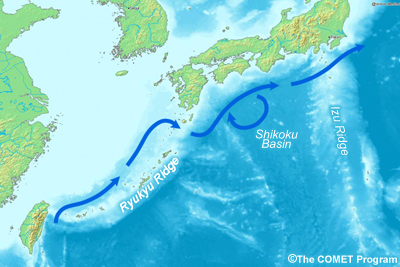
Not all eddies form when they break off of overextended meanders. Some result when bathymetry deflects a current. This example shows a semi-permanent eddy that forms south of Japan along the Kuroshio Current. The Kuroshio passes through a gap in the Ryukyu Ridge and follows a curved path through the deep Shikoku Basin, before exiting through a gap in the Izu Ridge. The current’s curved path through the basin initiates a clockwise-spinning (anticyclonic) eddy.
Oceanography from Models » Ocean Phenomena » Upwelling
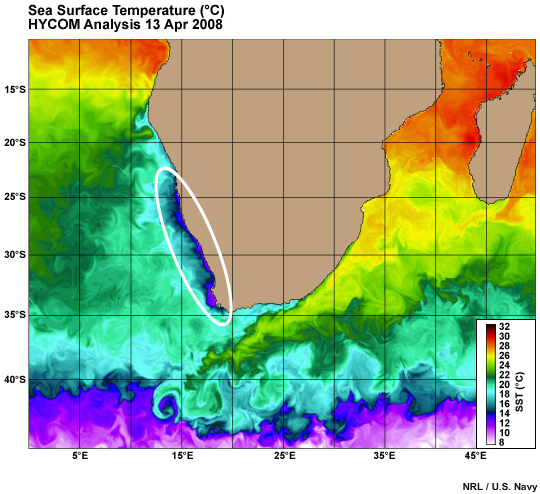
Upwelling occurs when cold, deep water is brought to the surface. It typically occurs along coasts or along the equator as a result of the Ekman process. Due to a balance between wind stress and the Coriolis Effect, the flow of wind across the surface will move surface water to the right in the Northern Hemisphere, or to the left in the Southern Hemisphere. The most obvious way find areas of upwelling it to look for areas with abnormally low sea surface temperatures.
Question 11
On the image below:
- Use the pen to outline a region of upwelling.
When you have finished, select Done.
Compare your answer to the answer below.
Please continue watching the video above.
In this example we see extensive upwelling along the southwest coast of Africa, shown in deep blue.
Question 12
From what direction are the prevailing winds blowing? (Choose the best answer.)
The correct answer is c) SSE.
Please continue watching the video above.
Because we are looking at the Southern Hemisphere, Ekman surface transport is to the left of the winds. This pushes surface water offshore and deeper water upwells to replace it. Similar upwelling occurs when a southerly wind blows parallel to the west coast of South America or when a wind from the north blows parallel to the California coast. As a reminder, note that meteorologists talk about winds from, while oceanographers discuss currents toward a direction.
Oceanography from Models » Ocean Phenomena » Upwelling and Plankton Blooms
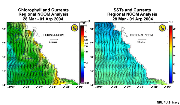
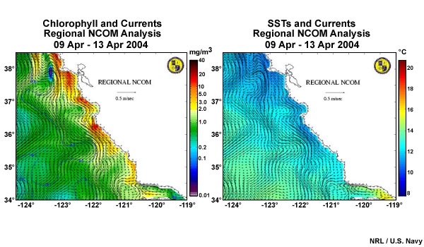
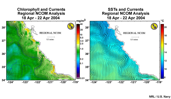
When this colder water rises from depths below the photic zone, where light does not penetrate, it carries a rich nutrient load. The combination of nutrients and light in shallow water leads to a bloom of phytoplankton, the base of the food chain. Thus, areas of frequent upwelling support large fisheries. This loop shows NCOM predictions of chlorophyll and sea surface temperature along the California coast covering a 3-week period before, during, and after a plankton bloom. Chlorophyll is the green pigment found in plants and phytoplankton. We can see that during the bloom, the coastal temperatures decrease due to upwelling while the chlorophyll content increases until plankton consume the nutrients.
Oceanography from Models » Ocean Phenomena » Upwelling and Plankton Blooms
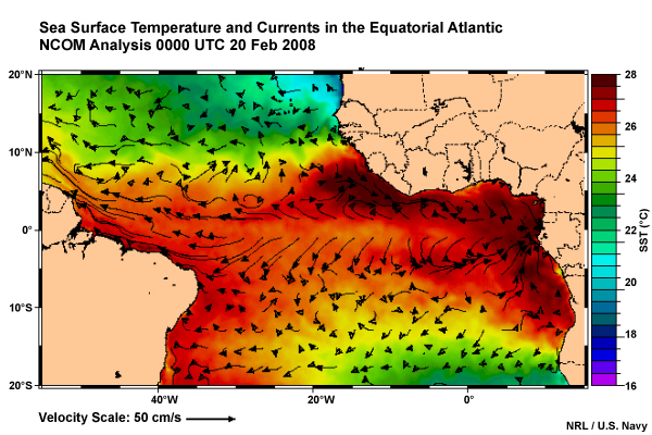
At the equator, the prevailing easterly winds blowing parallel to the equator cause ocean divergence at the surface. This happens because Ekman transport is to the right in the Northern Hemisphere and to the left in the Southern Hemisphere. This image shows current vectors plotted over sea surface temperatures for the equatorial Atlantic. Notice the strong divergence in currents along the equator and the lower (more yellow) sea surface temperature that results.
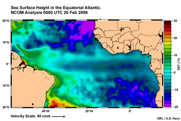
This upwelling of cooler deep water also results in a pronounced trough in sea surface height along the equator.
Oceanography from Models » Ocean Phenomena » Internal Tides
Internal tides refer to tidally generated waves that propagate through the ocean, but below the surface. Just like wind waves at the surface, their restoring force is gravity. But instead of travelling along the sea surface, they travel along surfaces where there is a strong vertical change in density, such as occurs in the thermocline at the base of the mixed layer. Internal waves are formed when tidally driven currents in the deep ocean slosh on and off the edge of the continental shelf, resulting in a back and forth horizontal motion over shallow bathymetric features like mid-ocean ridges that generate these waves. The resulting internal tidal waves tend to have long, diurnal (24 hour) or semidiurnal (12 hour) periods.
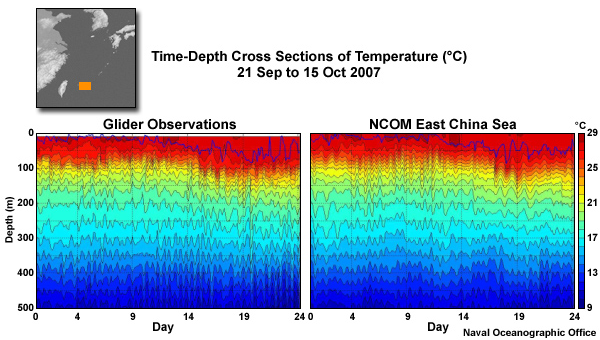
These graphics show time versus depth cross sections of water temperature for a location in the western Pacific during a 24-day period. Contours on the plot are isotherms, or surfaces of constant temperature. The plot on the left was created using glider observations while the plot on the right was created with the high-resolution East China Sea – Navy Coastal Ocean Model. The squiggles in the isotherms represent internal tides. The heavy purple line near the surface indicates the depth of the mixed layer.
Question 13
What is the approximate amplitude (trough to crest) of the largest waves? (Choose the best answer.)
The correct answer is b) 50 m.
Please continue watching the video above.
>Note that in the plot of glider observations on the left, the waves reach amplitudes of 50 m. Toward the end of the period, waves exceeding 50 m appear to occur quite close to the surface.
Question 14
What is the average period of the waves? (Choose the best answer.)
The correct answer is b) 12 hours.
Please continue watching the video above.
If you pick an isotherm with relatively well defined waves and count the peaks in a 5 day period, you should come up with something close to 10 peaks. That indicates 2 peaks per day, or a period close to 12 hours.
Internal tides are operationally important for several reasons. First, the depth of the mixed layer can rise and fall substantially in response to internal tides. This has important implications for ocean acoustics, as we discuss later in this module. Second, internal tides generated in regions with large tidal ranges can lead to strong undersea currents. These can severely impact structures such as offshore oil platforms. Third, internal tides are now thought to provide a mechanism for mixing deep-ocean water that was previously not considered important.
Oceanography from Models » Ocean Phenomena » Questions
Question 15
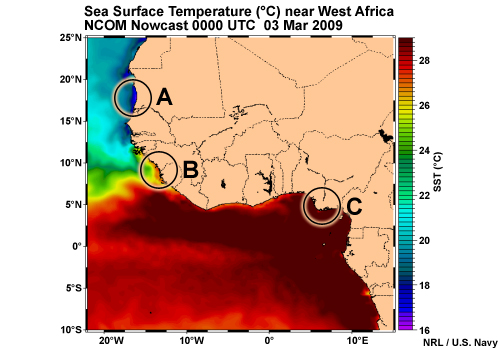
This map shows sea surface temperature along the west coast of Africa. Which location appears to experience upwelling? (Choose the best answer.)
The correct answer is A.
Upwelling results in cooler sea surface temperatures at the surface as deeper, cooler water is drawn to the surface. Location A shows cooler temperatures right along the coast. As there doesn’t appear to be any way those cooler waters could have advected into the area, we can conclude that they result from upwelling.
Question 16
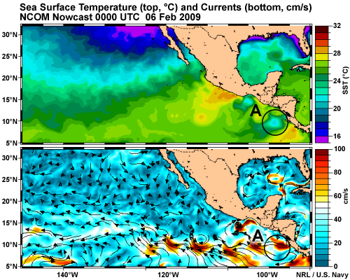
Look at these maps of currents and sea surface temperature. What process is occurring at location A? (Choose the best answer.)
The correct answer is d) upwelling.
The sea surface temperature analysis shows cooler temperatures at location A. These temperatures are consistent with either upwelling or formation of a cold core eddy. However, the current analysis does not show eddy circulation. Instead, it shows water flowing offshore, away from the coast, most likely driven by winds at the surface. These temperatures and currents are consistent with coastal upwelling.
Question 17
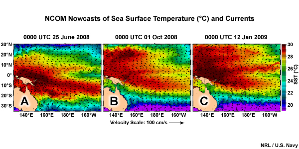
These maps show temperature and currents at the sea surface in the western Pacific Ocean. Which one most likely indicates equatorial upwelling? (Choose the best answer.)
The correct answer is A.
All three analyses show depressed temperatures at the surface along the equator. However, advection of cold water from coastal South America can also cause this feature. Map A also shows divergent surface currents that are a signature of equatorial upwelling. Viewing cross sections across the equator could confirm this interpretation.
Applications
There are many ways to apply ocean models in operations. In this section we explore some of those applications.
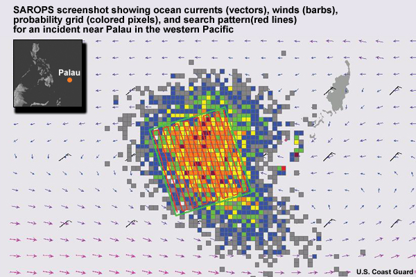
Applications » Search and Rescue (SAR)
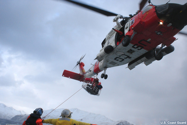
The U.S. Coast Guard (USCG) and Navy are frequently called upon to conduct search and rescue (SAR) operations in the offshore waters anywhere in the world. To assist in these operations they use SAROPS search tracking software. SAROPS combines a database of drift characteristics of different objects (people, sailboats, ships, etc) along with model forecasts of surface winds and ocean currents.
The U.S. Coast Guard (USCG) and Navy are frequently called upon to conduct search and rescue (SAR) operations in the offshore waters anywhere in the world. To assist in these operations they use SAROPS search tracking software. SAROPS combines a database of drift characteristics of different objects (people, sailboats, ships, etc) along with model forecasts of surface winds and ocean currents.
Applications » Optimal Track Ship Routing (OTSR)
As is implicit in the name, optimal track ship routing (OTSR) seeks to find the most efficient route for ships across the ocean. Ideally OTSR results in a safer passage and quicker arrival, saving money, lives, and property. The optimal track will take advantage of currents to speed passage and conserve fuel, while avoiding hazards such as storms. Thus, OTSR utilizes currents from ocean models and winds from weather models.
Question 18
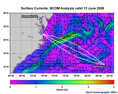
To see how this might work, imagine that you are on a sailboat participating in the annual Bermuda Ocean Race from Annapolis, MD, to the island of Bermuda held in mid-June. Using the currents shown in this figure, but ignoring winds, which of the following routes is likely to be the fastest? (Choose the best answer.)
The correct answer is a).
Please continue watching the video above.
In the 2008 Annapolis to Bermuda race, the winning boats in the three fastest classes followed a path that stayed in the Gulf Stream for the longest distance, well north of the straight line route from Chesapeake Bay to Bermuda, much like the route (a) shown here.
Applications » Ocean Heat Content and Hurricanes

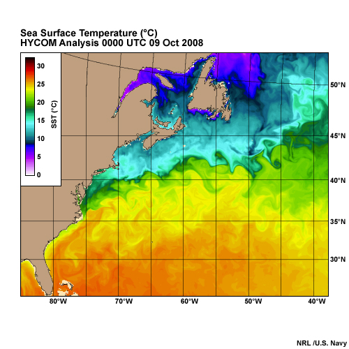
Tropical cyclones feed on surface water temperatures of 26°C or greater. That is, these storms extract their energy from the heat of the ocean water. For example, this plot shows a HYCOM analysis of SSTs in the Gulf of Mexico just prior to Hurricane Ivan in 2005. Now, if the SST were below 26°C, we would expect the cyclone to weaken. However it is possible for a hurricane to pass over an area of very warm SSTs and still weaken if that warm water is only a shallow surface layer.
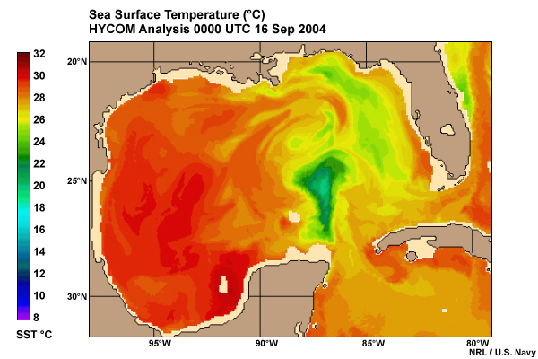
This occurs because strong hurricane winds can mix the warm surface water with deeper cooler water so that the surface water cools below the 26°C threshold. This plot shows a HYCOM analysis of SSTs just after Hurricane Ivan. The intensity of Ivan decreased from a category 5 to category 3 as it crossed the Gulf of Mexico.
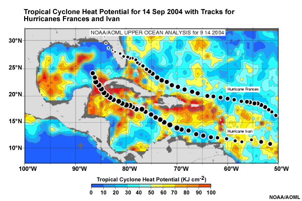
A better way to look at the potential for hurricane intensification is to look at ocean heat content. Regions with high SSTs and high ocean heat content are much more likely to sustain hurricanes than areas with high SSTs but low ocean heat content.
Ocean Heat Content reflects the energy excess in water above 26°C integrated through the water column down to a depth where the temperature falls below 26°C. Thus a temperature profile with a very shallow layer of warm surface might have an ocean heat content less than a column of water with a deep layer of water that only slightly exceeds 26°C.
If you look at the ocean heat content as Ivan entered the Gulf, you can see that most of its northward path was over areas with relatively low ocean heat content, despite the high SST. This undoubtedly contributed to Ivan’s loss of intensity as it crossed the Gulf.
Applications » Tracking Oil Spills
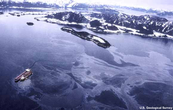
In 1989, the Exxon Valdez ran aground on Bligh Reef in Prince William Sound, Alaska, and spilled 11 million gallons of crude oil.
In order to track the trajectory of the spilled oil, the Hazardous Material (HAZMAT) response teams at NOAA and elsewhere rely on GNOME (General NOAA Operational Modeling Environment). GNOME helps to predict (a) how wind and currents might move and spread the oil and (b) how the oil changes chemically and physically as it weathers during the time it stays at the sea surface. GNOME uses current and temperature data from an ocean model as part of its initial conditions.
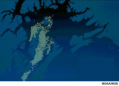
Applications » Tracking Ocean Creatures - Sea Nettles
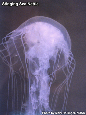
Sea Nettles are a stinging Jellyfish found along the East Coast of the U.S., particularly in brackish water close to rivers and estuaries. In Chesapeake Bay, stings from Sea Nettles can be particularly painful and thus have an enormous economic impact in summer months when crowds normally flock to the beach.
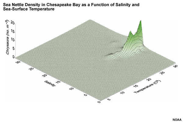
By studying the water conditions where Sea Nettles occur, biologists determined that the range of temperature and salinity they prefer is actually quite narrow. This plot shows the abundance of Sea Nettles by salinity and temperature. A narrow peak occurs at salinities around 15 parts per thousand and temperatures warmer than about 20°C.
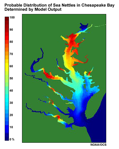
These biologists have worked with oceanographers to develop a model that combines the temperature and salinity conditions with the Sea Nettle distribution to determine the likelihood that a swimmer will encounter them at a given location. In this figure, that likelihood ranges from near zero, shown in dark blue, to nearly 100% in dark red. This particular model will provide predictions out to 3 days, plenty of time to plan for the weekend.
Applications » Ocean Acoustics
Ocean acoustics, that is, the way that sound travels underwater, has surprisingly important applications. From the civilian side, ocean acoustics impact seafloor surveying, offshore oil exploration, marine mammal conservation, and all manner of oceanographic research. On the national defense side, ocean acoustics play a pivotal role in locating and communicating with submarines and other submersibles.
Applications » Ocean Acoustics » Principles of Ocean Acoustics
The properties that determine underwater sound speed and acoustic range are temperature, salinity, and pressure – ocean properties that are predicted by ocean circulation models.
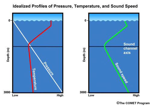
Sound speed increases with increasing temperature, salinity, and pressure. If we combine these relationships with some knowledge of the vertical structure of the ocean, we can come up with a vertical profile of sound speed in the ocean, like that shown here.
Applications » Ocean Acoustics » Sound Refraction
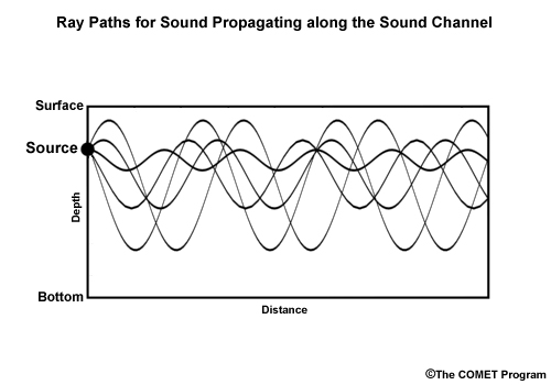
Through the process of refraction, sound waves bend toward areas of slower speed. The result is that sound waves emanating from a source, either at the surface or below, do not uniformly radiate outward. For example, the sound speed minimum near the base of the thermocline leads to a sound channel that traps sound waves. This graphic shows sound ray paths for a source within this sound channel. Sounds that originate within this layer are constantly bending back toward the sound speed minimum without dissipation. As a result, these sounds can be heard for thousands of miles across the ocean.
Applications » Ocean Acoustics » Horizontal Variations in Sound Speed
In addition to vertical variations, sound speed also varies horizontally. These horizontal variations are particularly large near ocean fronts that separate warm and cold bodies of water. Therefore, features like the north wall of the Gulf Stream or current rings and eddies have significant effects on sound transmission. Submarine captains use this information to hide near ocean fronts. With good predictions of temperature and salinity, we can determine sound travel underwater across these structures.
Applications » Subsurface Operations
Many marine operations occur underwater. Subsurface currents obviously have a direct impact on planning and conducting these operations. However, subsurface currents are difficult to detect and measure. They may run counter to surface currents, even at relatively shallow depths. For our best predictions, we must rely upon ocean models.
Question 19
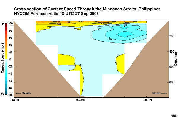
This plot shows a HYCOM forecast of current velocity in a cross section across the Straits of Mindanao in the Philippines. The cross section is oriented north-south and positive current speeds are directed eastward, while negative speeds are oriented westward. Units are cm/s.
Use the pull-down menu to choose the best answer.
The correct answers are highlighted above.
Please continue watching the video above.
Surface current speeds have positive values, so they are flowing toward the east. At a depth of 200 m, currents have negative values, indicating westward flow. Note that the zero contour lies at a depth of as little as 50 m in the northern part of the cross section, with tightly packed contours above and below. For a shallow submersible, this could dictate exactly how deep you choose to go.
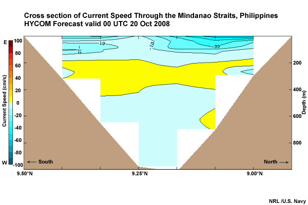
Now compare the previous cross section to this one, 25 days later. Note that surface currents are directed westward while currents at a depth of 200 to 400 meters, while weak, are directed to the east. This sort of variability will not be reflected in climatologies of ocean currents.
Applications » Questions
Question 20
Which of the following properties does SAROPS use to predict object drift? (Choose all that apply.)
The correct answers are a) and b).
SAROPS combines a database of drift characteristics of different objects (people, sailboats, ships, etc) along with model forecasts of surface winds and ocean currents.
Question 21
GNOME is used for which of the following applications? (Choose the best answer.)
The correct answer is c).
GNOME helps to predict (a) how wind and currents might move and spread the oil and (b) how the oil changes chemically and physically as it weathers during the time it stays at the sea surface. GNOME uses current and temperature data from an ocean model as part of its initial conditions.
Question 22
Why can the distribution of Sea Nettles be predicted using ocean models? (Choose the best answer.)
The correct answer is b).
Biologists have determined that the range of temperature and salinity Sea Nettles prefer is actually quite narrow: salinities around 15 parts per thousand and temperatures warmer than about 20°C.
Question 23
Sound waves bend toward areas of slower sound speed. (Choose the best answer.)
The correct answer is True.
Through the process of refraction, sound waves bend toward areas of slower speed. The result is that sound waves emanating from a source, either at the surface or below, do not uniformly radiate outward. For example, the sound speed minimum near the base of the thermocline leads to a sound channel that traps sound waves.
Operational Ocean Models
| Model | Areal Extent |
Vertical Coordinates |
Layers | Horizontal Resolution |
Horizontal Grid |
|---|---|---|---|---|---|
| NLOM | Global | Density Layers |
7 | 1/32° (3.5 km/2 nm) |
Regular |
| NCOM (Global) |
Global | Sigma-Z | 41 | 1/8° (14km/7.5 nm) |
Regular |
| NCOM (Hi-Res) |
Regional | Sigma-Z | 51 | 1/36° (3km/1.7 nm) |
Regular |
| HYCOM | Global | Sigma-Z- Density |
Varies (>40) |
1/12° (9 km/5 nm) |
Regular |
| SWAFS | Regional | Sigma | 27-47 | 1/50° (2.2 km/1.2 nm) |
Regular |
| ADCIRC | Regional | Sigma | Varies | Varies | Finite Element |
The U.S. Navy and NOAA run several operational ocean circulation models. These are physics-based fluid dynamics models that resolve mesoscale features including fronts and eddies. The Navy models are forced by FNMOC wind and heat fields.
Each of the models can be classified by its horizontal and vertical coordinate schemes along with the areal extent it was designed to cover. Here we briefly describe each of the five operational models currently in use.
Operational Ocean Models » Navy Layered Ocean Model (NLOM)
NLOM is a global circulation model run with a relatively high resolution of 1/32° (3.5 km/2 nm). Horizontally, it uses a rectangular or curvilinear grid. Vertically, it only has a mixed surface layer underlain by 6 deep-water layers determined by seawater density. It was developed to forecast surface elevation structure, along with the locations of fronts and eddies and is used to initialize the Global NCOM. NLOM is only valid for offshore waters deeper than 200 meters. That is why there is no data on the continental shelf in the example shown here.
Operational Ocean Models » Navy Coastal Ocean Model (NCOM)
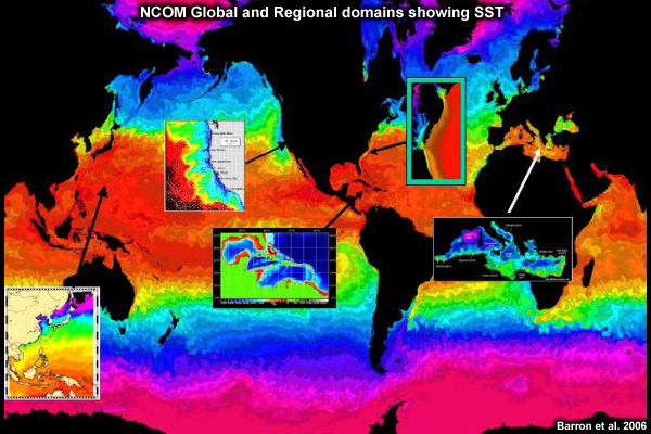
NCOM is a circulation model run in two different implementations: global and high-resolution. This image shows sea surface temperatures for the global domain along with several regional domains. All implementations are based on the Princeton Ocean Model (POM). Horizontally, NCOM uses rectangular or curvilinear grids. Vertically, it uses sigma (bottom-following) coordinates in shallow water and depth-based (z) coordinates in deep water.
The global NCOM covers the globe but the Naval Oceanographic Office publishes products from 60°S to 75°N. This is a deep-water model run at a resolution of 1/8° (14km/7.5 nm) and 41 vertical levels. Because the model is designed for deep water, data within 3 grid-points of shore (~42 km) should be used with extreme caution. In 2010, global NCOM will be replaced by the Hybrid Coordinate Ocean Model (HYCOM).
The High-Resolution Navy Coastal Ocean Model (HIRES-NCOM) is for ocean areas with approximate dimensions of 15° x 15° (1600 x 1600 km). It is run with a resolution of 1/36° (3km/1.7 nm) and 51 vertical levels. NAVOCEANO plans to implement a total of 16 high-resolution domains around the world. Global NCOM and higher-resolution COAMPS winds provide the initial conditions.
Operational Ocean Models » Hybrid Coordinate Ocean Model (HYCOM)
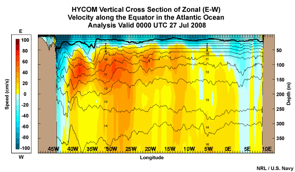
HYCOM is another global circulation model. At the Navy, it will eventually replace the global NCOM. Like NCOM, HYCOM is based on the Princeton Ocean Model (POM) and uses a similar horizontal coordinate scheme with a resolution of 1/12° (9 km/5 nm). HYCOM combines 3 vertical coordinate systems: z-level coordinates near the surface in the mixed layer, terrain-following sigma coordinates in shallow coastal regions, and density (isopycnal) coordinates in deep water below the mixed layer. This cross section of current velocity across the equatorial Atlantic also shows the vertical layers used in the model.
HYCOM is the operational model at NCEP. They use an implementation of HYCOM in the northwest Atlantic called the Real-time Ocean Forecast System (RTOFS) – Atlantic. A number of other national oceanographic centers, outside of the U.S., also run HYCOM.
Operational Ocean Models » Shallow Water Analysis and Forecasting System (SWAFS)
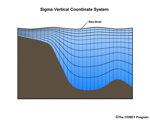
SWAFS is a regional circulation model, also based on the Princeton Ocean Model. It uses regular horizontal grids with a resolution up to 1/50° (2.2 km/1.2 nm). Vertical coordinates throughout the domain are terrain-following sigma coordinates, like those shown here. SWAFS is being replaced with high-resolution NCOM.
Operational Ocean Models » Advanced Circulation Model (ADCIRC)
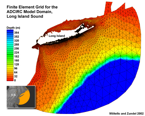
In littoral and nearshore regions, ADCIRC provides high-resolution forecasts of tidal and estuarine elevations and currents. With tidal forcing only (no winds), ADCIRC can potentially forecast months into the future. ADCIRC uses sigma vertical coordinates while horizontally, it uses a finite element approach with triangular nodes, like those shown here. This allows short spacing with horizontal resolutions of meters when there are complicated features (channels, beaches, underwater ridges, etc.), while spacing for flat bottoms can be 100m-10km. This allows ADCIRC to efficiently simulate processes over complex bathymetry and along coastlines, inlets, and beaches. With proper bathymetry and coastal topography, ADCIRC can forecast tidal wetting and drying, storm surge, and inundation.
Operational Ocean Models » Other Ocean Circulation Models
There are many more ocean circulation models. Some are operational models run by other countries, like MERCATOR in France or FOAM in Britain. Others are research models run by the academic community, like the Princeton Ocean Model. A list of the most common models, along with appropriate links, is available in the reference section of the module.
Operational Ocean Models » Questions
Question 24
Which of the following ocean models uses a mixed surface layer underlain by 6 deep-water layers determined by density? (Choose the best answer.)
The correct answer is c) NLOM
Vertically, NLOM has a mixed surface layer underlain by 6 deep-water layers determined by seawater density. It was developed to forecast surface elevation structure, along with the locations of fronts and eddies.
Question 25
Which of the following ocean models combines 3 vertical coordinate systems: z-level coordinates, terrain-following sigma coordinates, and density coordinates? (Choose the best answer.)
The correct answer is a) HYCOM.
HYCOM combines 3 vertical coordinate systems: z-level coordinates near the surface in the mixed layer, terrain-following sigma coordinates in shallow coastal regions, and density (isopycnal) coordinates in deep water below the mixed layer.
Question 26
Which of the following ocean models will be replaced by the Hybrid Coordinate Ocean Model (HYCOM)? (Choose the best answer.)
The correct answer is b) NCOM.
In 2010, global NCOM will be replaced by the Hybrid Coordinate Ocean Model (HYCOM).
Question 27
Which of the following ocean models uses a horizontal finite element approach with triangular nodes? (Choose the best answer.)
The correct answer is a) ADCIRC.
ADCIRC A finite element approach with triangular nodes allows short spacing with horizontal resolutions of meters when there are complicated features (channels, beaches, underwater ridges, etc.), while spacing for flat bottoms can be 100m-10km. This allows ADCIRC to efficiently simulate processes over complex bathymetry and along coastlines, inlets, and beaches.
Summary
Mesoscale ocean circulation models simulate temperature, salinity, currents, and elevation in 3 dimensions through a period of time. These models have sufficient resolution to simulate mesoscale processes, like eddy formation and dissipation.
Models make several assumptions in order to simplify computations, deal with processes that can’t be modeled, and run efficiently. These assumptions lead to several limitations:
- Numerical errors stem from parameterization and the use of discreet time steps and grid spacing.
- Post-processing limits the amount of information available to us.
- Observations used to initialize models suffer from sparseness and measurement errors.
- NWP models used to initialize models also suffer from their own suite of errors.
- All model predictions degrade with time.
Mesoscale ocean circulation models allow us to examine many ocean structures both at the surface and at depth, including the following:
- Current systems
- Ocean fronts
- Ocean eddies
We can also use models to study many processes, such as the following:
- Eddy formation and dissipation
- Upwelling
- Internal tides
The predictions provided by mesoscale ocean circulation models have many applications:
- Search and Rescue (SAR)
- Optimal Track Ship Routing (OTSR)
- Ocean Heat Content and Hurricane Forecasting
- Tracking Oil Spills and other hazardous materials
- Tracking Sea Nettles and other biological hazards
- Ocean Acoustics
- Subsurface Operations
References
Barron, C. N., A. B. Kara, R. C. Rhodes, C. Rowley, L. F. Smedstad, 2006: Validation Test Report for the 1/8 Global Navy Coastal Ocean Model Nowcast/Forecast System. NRL Tech Report, NRL/MR/7320--07-9019 https://www7320.nrlssc.navy.mil/pubs/2007/Barron-2007.pdf
Chesapeake Bay Sea Nettle Forecast Guidance
https://ocean.weather.gov/Loops/SeaNettles/prob/SeaNettles.php
Global Argo Data Repository (https://www.nodc.noaa.gov/argo/index.htm)
GNOME (General NOAA Operational Modeling Environment)
https://response.restoration.noaa.gov/oil-and-chemical-spills/oil-spills/response-tools/gnome.html
Marhoffer, W.R., Maritime Mass Rescue Operations [retrieved 24 Feb 2009 from http://www2.faa.gov/news/conferences_events/pacific_aviation/agenda/media/Mass_
Rescue_Operations_Planning.pdf]
Shay, L. K., Halliwell, G., Brewster, J., Lozano, C., Teague, W.: Evaluation and Improvement of
Ocean Model Parameterizations for NCEP Operations [retrieved 24 Feb 2009 from
https://www.nhc.noaa.gov/jht/ihc_08/s06-05shay_halliwell_session6_Ivan_.pdf]
Underwater Acoustics Tutorial [retrieved 24 Feb 2009 from
https://www.pmel.noaa.gov/vents/acoustics/tutorial/tutorial.html]
Operational Ocean Circulation Models
Global NLOM Nowcast/Forecast (https://www7320.nrlssc.navy.mil/global_nlom/)
Global NCOM Nowcast
(https://www7320.nrlssc.navy.mil/global_ncom/)
Global HYCOM Nowcast
(https://www7320.nrlssc.navy.mil/GLBhycom1-12/skill.html)
Naval
Oceanographic Office (https://www.usno.navy.mil/NAVO)
NOAA Real-Time Ocean
Forecast System - Atlantic ( https://polar.ncep.noaa.gov/ofs/)
Ocean Circulation Models
The following list of ocean circulation models is classified primarily on the basis of horizontal and vertical coordinate schemes.
- Finite difference schemes (Horizontal coordinates: regular, structured, rectangular,
curvilinear, etc)
- Z-based (depth) vertical coordinates
- Immiscible layers ("layered" models)
- Navy Layered Ocean Model NLOM
- Miami Isopycnic Coordinate Ocean Model, MICOM
- Hallberg Isopycnic Model, HIM
- Terrain-following vertical coordinates ("sigma" coordinate models)
- Princeton Ocean Model, POM
- Regional Ocean Modeling System, ROMS
- Terrain-following Ocean Modeling System TOMS
- Finite element schemes
- A. Triangular finite elements
- Advanced Circulation Model (ADCIRC)
- B. Spectral finite elements
- Spectral Element Ocean Model (SEOM)
- A. Triangular finite elements
- Finite volume methods
- Finite Volume Community Ocean Model (FVCOM)
- Hybrid vertical coordinates (Finite difference)
Contributors
COMET Sponsors
The COMET® Program is sponsored by NOAA National Weather Service (NWS), with additional funding by:
- Air Force Weather (AFW)
- Australian Bureau of Meteorology (BoM)
- European Organisation for the Exploitation of Meteorological Satellites (EUMETSAT)
- Meteorological Service of Canada (MSC)
- National Environmental Education Foundation (NEEF)
- National Polar-orbiting Operational Environmental Satellite System (NPOESS)
- NOAA National Environmental Satellite, Data and Information Service (NESDIS)
- Naval Meteorology and Oceanography Command (NMOC)
Project Contributors
Principal Science Advisors
- Dr. Frank Bub - Ocean Models Tech Lead, Ocean Predictions Department (NP1M) Naval Oceanographic Office (NAVOCEANO)
Project Lead/Instructional Design
- Dr. Alan Bol - UCAR/COMET
Graphics/Interface Design
- Steve Deyo - UCAR/COMET
- Brannan McGill - UCAR/COMET
Multimedia Authoring
- Dan Riter - UCAR/COMET
Audio Editing/Production
- Seth Lamos - UCAR/COMET
Audio Narration
- Tia Marlier
COMET HTML Integration Team 2021
- Tim Alberta — Project Manager
- Dolores Kiessling — Project Lead
- Steve Deyo — Graphic Artist
- Ariana Kiessling — Web Developer
- Gary Pacheco — Lead Web Developer
- David Russi — Translations
- Tyler Winstead — Web Developer
COMET Staff, January 2009
Director
- Dr. Timothy Spangler
Deputy Director
- Dr. Joe Lamos
Administration
- Elizabeth Lessard, Administration and Business Manager
- Lorrie Alberta
- Michelle Harrison
- Hildy Kane
Hardware/Software Support and Programming
- Tim Alberta, Group Manager
- Bob Bubon
- James Hamm
- Ken Kim
- Mark Mulholland
- Wade Pentz, Student
- Jay Shollenberger, Student
- Malte Winkler
Instructional Designers
- Dr. Patrick Parrish, Senior Project Manager
- Dr. Alan Bol
- Lon Goldstein
- Bryan Guarente
- Dr. Vickie Johnson
- Tsvetomir Ross-Lazarov
- Marianne Weingroff
Media Production Group
- Bruce Muller, Group Manager
- Steve Deyo
- Seth Lamos
- Brannan McGill
- Dan Riter
- Carl Whitehurst
Meteorologists/Scientists
- Dr. Greg Byrd, Senior Project Manager
- Wendy Schreiber-Abshire, Senior Project Manager
- Dr. William Bua
- Patrick Dills
- Dr. Stephen Jascourt
- Matthew Kelsch
- Dolores Kiessling
- Dr. Arlene Laing
- Dr. Elizabeth Mulvihill Page
- Amy Stevermer
- Warren Rodie
- Dr. Doug Wesley
Science Writer
- Jennifer Frazer
Spanish Translations
- David Russi
NOAA/National Weather Service - Forecast Decision Training Branch
- Anthony Mostek, Branch Chief
- Dr. Richard Koehler, Hydrology Training Lead
- Brian Motta, IFPS Training
- Dr. Robert Rozumalski, SOO Science and Training Resource (SOO/STRC) Coordinator
- Ross Van Til, Meteorologist
- Shannon White, AWIPS Training
Meteorological Service of Canada Visiting Meteorologists
- Phil Chadwick
- Jim Murtha