EPS Products Reference Guide »
Extreme Forecast Index and Shift of Tails
Description
The Extreme Forecast Index (EFI) and Shift of Tails (SOT) product is used to evaluate the possibility of weather variables having unusual or extreme values compared to a model climate. Forecasters are not always familiar with what constitutes a typical range of conditions based on model output only. Therefore, a comparison to the model climate (or observed climatology in some products) is useful to help identify anomalous forecast conditions that could cause significant weather impacts.
Interpretation
The EFI and SOT are produced by comparing the current ensemble forecast data with those from a model climate, or “M-climate.” The M-climate usually consists of an ensemble of re-forecasts for several days or a few weeks around the current date, which are run using re-analyses or initial conditions for the most recent 20 to 30 years.
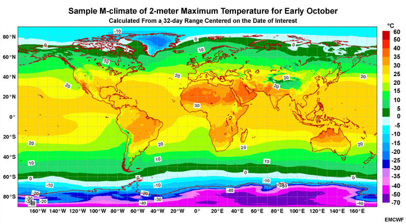
The resulting model climate gives a picture of the model’s usual range of conditions at a given location, time of year, and forecast lead time (24-48 hours), even where surface or other observations are limited. The M-climate can then be used to gauge whether current events are anomalous without defining specific thresholds.
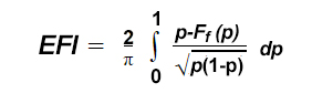
The EFI value is a function of the integral of the difference between the current ensemble cumulative distribution function (CDF) and the M-climate CDF, or the area between the two CDFs. The values of EFI range from -1 to 1.
When the model climate and ensemble CDF are exactly the same or spread evenly about the median, the EFI equals zero. This rarely happens so you are likely to see one of the following situations.
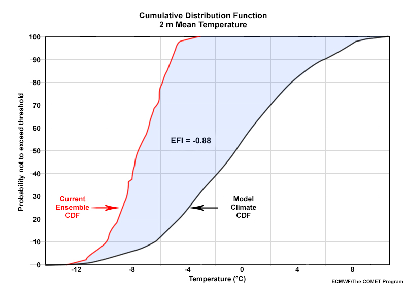
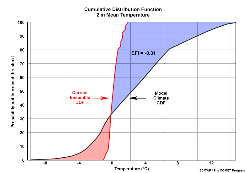
When the values in the current ensemble CDF are significantly lower than those of the model climate, the EFI is negative. We see that above.
When the values in the ensemble CDF are well above those of the model climate, the EFI is positive (shown below).
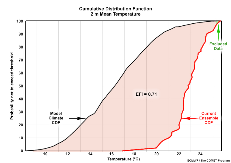
Be aware that the EFI will not represent the full measure of the anomaly when the current ensemble CDF of forecast values lies partially outside the range of the model climate (as seen above). The green area at the upper tail of the ensemble CDF line extends slightly past the model climate CDF line and is not included in the EFI value.
Other configurations are also possible. One part of an ensemble forecast CDF may have lower values than the model climate CDF while the rest has higher values. In this case, the positive and negative contributions cancel somewhat, bringing the EFI closer to zero.
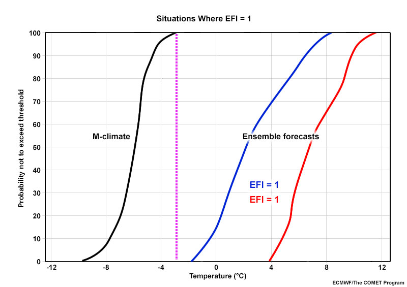
There are two other possibilities for EFI values: -1 and 1. Here, all of the current ensemble forecast values are either lower or higher than the range of the model climate, respectively.
Importantly, we cannot tell how far the current ensemble CDF extends beyond the M-climate range: if it is well outside it or only a little beyond. That’s where the Shift of Tails (SOT) parameter comes in. It shows how far the upper and lower tails of the ensemble distribution are from the model climate’s limits.
The SOT is a ratio of the difference between the ensemble 90th percentile and model climate 99th percentile, A, compared to the difference between the model climate 99th and 90th percentiles, B. A graphical representation of the SOT calculation is shown below.
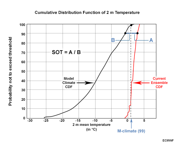
If the SOT value is positive, the tail of the ensemble distribution is likely to be higher than the range of the model climate. If the SOT value is negative, the ensemble distribution extends to lower values than the model climate range. The larger the SOT value, the further outside the model climate range the tail of the ensemble distribution lies.
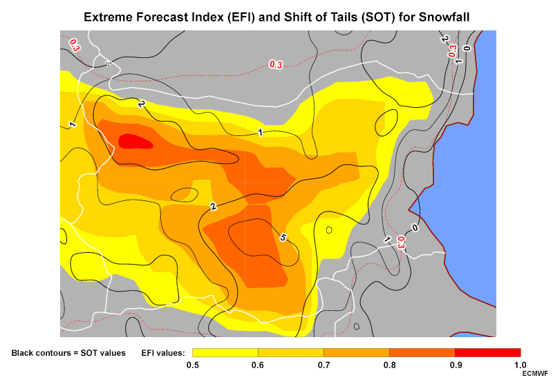
In the plan-view example below, EFI greater than 0.5 is colour-shaded according to the legend while SOT values are contoured in black. EFI values between 0.5 and 0.8 (irrespective of sign) are generally considered unusual. EFI values between 0.8 and 1 (irrespective of sign) are considered very unusual or extreme.
Thus, the red bulls-eye of 0.9-1.0 in the upper left indicates extreme forecast snowfall amounts compared to the model climate. The dark orange area extending southward indicates unusually high amounts.
High values of SOT ranging from 2 to 5 coincide with these areas of EFI value. This means that the tail of the ensemble distribution is higher than the model climatology by a fair amount and that extreme amounts are present within the distribution across these regions.
Strengths & Weaknesses
Strengths:
- The EFI and SOT let you quickly anticipate anomalous weather conditions. They are especially useful for assessing whether severe events are possible in the medium-range forecast period.
- They use a model climate, which provides more comprehensive coverage over the entire globe than an observed climatology with gaps in spatial coverage or historical records.
- Current model biases are accounted for within the model climate itself, reducing the need to take model bias into account when using the product.
Weaknesses
- The EFI and SOT do not show the type of weather or details of weather systems—only whether specific forecast variables are anomalously high or low compared to the model climate.
- They do not show the shape of the ensemble distribution—if it is normal, multimodal, or clustered. You can only guess at the CDF (and thus the PDF) unless you query the underlying data further.
- The model climate is not equivalent to observed climatology and may capture more or less than the full range of possible conditions at a given location.
Effective Use
EFI and SOT maps are useful for quickly assessing whether anomalously strong weather systems or conditions are possible in the forecast period. But they do not show ensemble differences in, for example, system timing or placement or the most likely outcomes or probabilities. This means that they should be used in combination with other plots in the following ways.
- Use a mean and spread map to help determine overall uncertainty within the ensemble system and refine whether there are differences in weather system timing, magnitude or placement to consider.
- Use a spaghetti plot or plume diagram to see the shape of the ensemble member distribution over space and time, respectively. This will let you identify clustering and assess whether the median and mean are representative of most likely outcomes. This can be especially important when the EFI value is low because part of the ensemble forecast CDF has lower values than the model climate CDF while the rest has higher values.
- Use probability of exceedance maps to understand whether specific values of interest (such as the freezing point) or other industry or warning criteria thresholds may be exceeded.
- View the individual model climate CDF and current ensemble CDF for a given EFI/SOT variable when they are available. They can help you understand the shape of the distributions and the reason for the EFI and SOT values. They can also help you understand how well the ensemble mean and median represent all of the members.
While the SOT is useful for understanding the extremes of the distribution (the upper and lower 10%), unusually high or low values compared to climatology (such as the 85th percentile) are important as well. So, it’s critical to consult other probabilistic information to understand the situation fully and deliver service relevant to various audiences.
Keep the following points in mind when using EFI and SOT maps.
- EFI is best used in the medium-range forecast period, from about 2-7 days. Beyond that, it usually tends toward 0 because of the high degree of spread in ensemble members.
- In areas with an EFI of 1 or -1 (fully outside the model climate distribution), examine the SOT carefully to estimate how far the ensemble forecast lies outside of the model climate distribution. Also consult the underlying CDFs or use another product with full distribution information.
- Due to the complexity of EFI and SOT values, they are generally best left out of public forecast statements.
- The model climatology is updated twice weekly so the switch in climatological calculation may cause inconsistent values between runs.
Examples, Part 1
Question 1 of 2
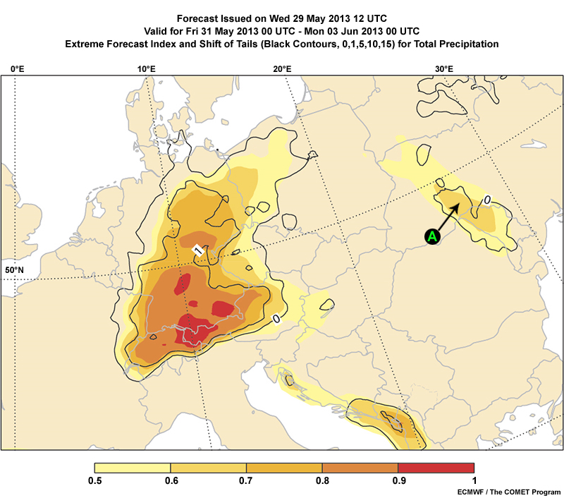
What are the values of the EFI and SOT at point A?
The correct answer is b.
Colour shading represents the EFI value. At point A, it is yellow-orange, which falls between 0.6 and 0.7. Black contours represent the SOT value. A single contour of 0 encompasses point A, with no contour of 1, so the SOT value is in the 0-1 range.
Question 2 of 2
An EFI of 0.6-0.7 suggests that the ensemble CDF contains higher values overall than those in the M-climate CDF. The slightly positive SOT suggests that the upper tail of the ensemble distribution lies slightly outside the M-climate range, leading us to expect an unusual or anomalously high precipitation event is possible. Extremely anomalous and/or record events usually occur with an EFI greater than 0.8 and a SOT greater than 5.
Examples, Part 2
Question 1 of 2
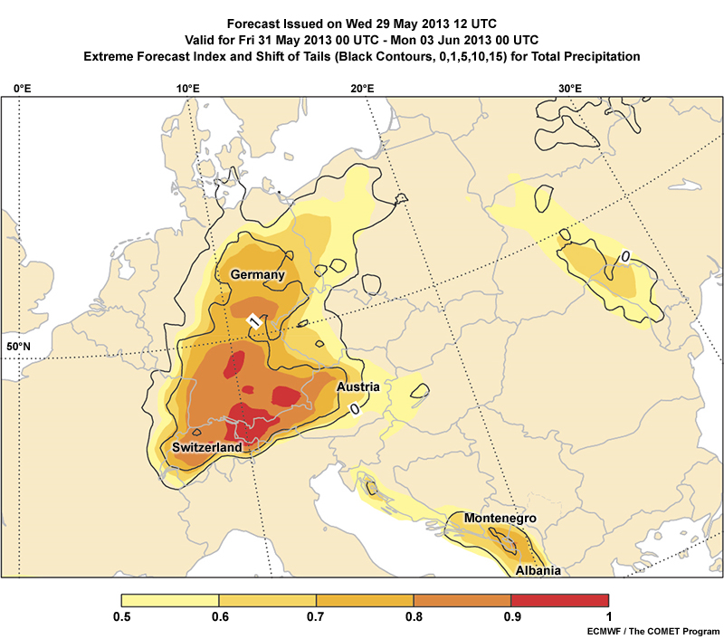
Based on the information in the graphic, where is the greatest amount of precipitation expected during the 4-day period?
The correct answer is d.
The map does not show how much precipitation will fall in any location. It only shows how unusual or extreme the member forecasts are compared to the model climate at that location and for that date range.
Question 2 of 2
What additional maps could help you easily estimate where the greatest amount of precipitation will fall during the 4-day period? (For those unfamiliar with the products listed below, probability of exceedance maps show the probability of exceeding a value of interest; mean and spread maps show the average value of a variable and a representation of its uncertainty; and plume diagrams show how a forecast variable changes over time at a location.)
The correct answers are b, c.
The model climate and current ensemble CDFs would help you gauge the shape of distribution and most likely outcomes, but not the placement of greatest precipitation.
Probability of exceedance maps can help you quickly identify areas in which certain amounts of precipitation are highly probable. Viewing several maps with increasing values can effectively narrow down the regions of high precipitation amounts.
Mean and spread maps of total precipitation can also help identify the areas in which the model generally predicts high amounts of precipitation. They also show the uncertainty in that mean calculation.
Plume diagrams are useful for gauging total precipitation amount at a specific location. However, they are usually available for select cities and do not allow you to quickly assess precipitation amounts over a large region.
Links
- NOAA ESRL, Precipitation Forecast Products Based on NCEP GEFS Reforecasts, Version2: https://www.esrl.noaa.gov/psd/forecasts/reforecast2/analogs/ (Change “Plot Type” to “Extreme Forecast Index, Percentiles” then click “Get Forecast”)
- Canadian Meteorological Centre (CMC) EFI for days 1 - 7: http://collaboration.cmc.ec.gc.ca/cmc/cmoi/cmc-prob-products/