EPS Products Reference Guide »
Ensemble Trajectories

Description

Ensemble trajectory plots show the forecast tracks of individual weather features from all ensemble members in one plan-view map. They can be generated for a variety of features, such as cyclonic vorticity centres, surface low or high pressure centres, tropical cyclones, and individual convective storm cells.

In this guide, we will focus on trajectories of surface low pressure centres since they are one of the most common EPS trajectory products, and are very similar to tropical cyclone tracks.

Interpretation

Low centre trajectory plots show the path of the estimated centre of surface low pressure systems over time. The centres can be for:

• A specific pressure value, such as 1000 hPa
• The lowest pressure value in a system
• The gradient wind vorticity maximum

Note that the magnitude of the low can only be derived when the centre is for the lowest pressure values.

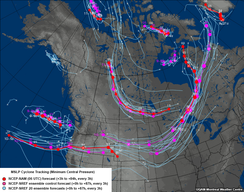
On the plot below, low pressure centre tracks are shown in teal. A deterministic run (red) and a control run (magenta) are also plotted with waypoints for context. The legend indicates what the plot shows, in this case the minimum central pressure.

Depending on the display, waypoints may be plotted hourly, daily, or for any increment in between. Some plots include date and time markings beside the waypoints while others use different waypoint symbols for each time.

If date/time markings are provided, you can estimate the speed of the system from the length of the trajectories between waypoints: the longer the distance, the faster the system is moving. Note that a trajectory can start after the beginning of the forecast period or stop before the end, so you should carefully scrutinize the plot when estimating the speed of a feature for all members.

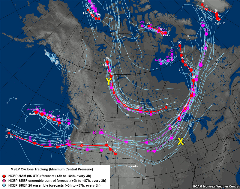
The distance between the different members’ waypoints (perpendicular to the track) also helps you understand the amount of spread in the distribution at a location or time. The greater the distance, the greater the uncertainty in forecast outcome. In this example, there is clearly more uncertainty in members at location X than location Y. However, there are tracks from multiple systems at location X, with the southern four trajectories from the system coming out of northeast Colorado. This is one of many reasons to be careful when use trajectories.

You can see the spatial maximum and minimum in the distribution by looking at the tracks on the outside of the group’s path or the outliers.

Sometimes a mean track is plotted. If not, you can get an idea of the most likely path (or paths if there is more than one cluster) by visually averaging the tracks.

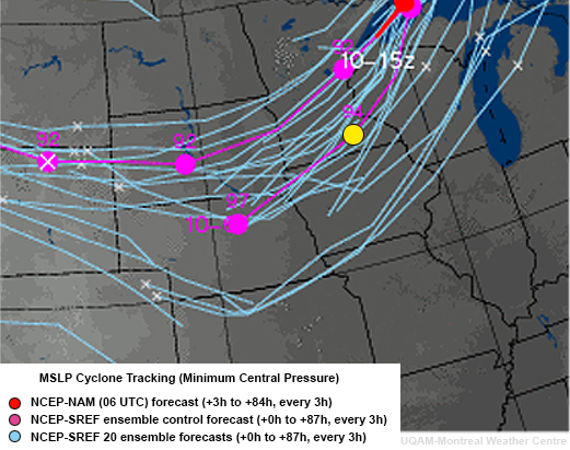
Occasionally, an EPS member will produce a distinct feature that is not present in the other members, such as the single low pressure track highlighted on the map above. In other cases, many, but not all, members will produce a feature. This becomes important when using low pressure system trajectory maps to gauge probabilities of the low’s position or timing. You’ll need to determine the number of members present and those that did or did not produce the feature. For example, to determine the probability that the low pressure system will track a specific way, you can count the number of members in a certain direction from the location of interest, then divide by the total number of members. The example below has 22 members, with 8 to the south of the yellow circle. This means that there’s a roughly 36% chance that the low will track to the south of that location.

Strengths & Weaknesses

Strengths:

• Ensemble trajectory plots show the full distribution of ensemble members, allowing you to estimate the shape of the distribution and presence of clustering. They also help you interpret the most likely outcomes (mean or median).
• The distance between members gives a general estimate of the spread and thus the uncertainty in the EPS solutions.
• The plots provide information about the position of the system; when waypoints are included, you can also estimate its timing.
• Unlike some other forms of ensemble output, feature tracking presents information in a way that’s highly compatible with other plan-view model data and observations, and with how forecasters conceptualize the development of weather systems.

Weaknesses:

• Plots may be difficult to read because of the high density of tracks.
• Differences in timing and location can be difficult to separate without waypoints.
• You can only assess the magnitude of a feature if the trajectories are plotted as the lowest central pressures.
• The low-centre algorithm or threshold may not exactly align with what you want to track. For example, a product may show 1000 hPa contours when you want to track lowest pressure positions.

Effective Use

Trajectory plots are useful for looking at all member solutions to estimate the shape of the distribution and general spread. When waypoints are included, they can be used to estimate differences in system timing.

Trajectory plots are best combined with other plots in the following ways.

• Use time-series of mean and spread plan-view mapsto determine differences in a feature’s timing versus location as well as its magnitude. They make it comparably easy to estimate the mean and uncertainty (spread). Consult one first to help you focus in on areas with higher uncertainty; this will let you add more value to the forecast there.
• Use plume diagrams to highlight timing differences in ensemble members, especially when the plan-view low track products do not contain waypoints.
• Use probability of exceedance/occurrence plan-view maps to estimate whether a threshold will be exceeded. That’s much easier than counting the tracks on one side of the location of interest.

Keep the following points in mind when using trajectory plots.

• Not all trajectories start at the beginning of the forecast period or stop before the end.
• When systems decay and have multiple low pressure centres around a main circulation, or when completely different systems cross the same location at different times, the clutter can become overwhelming and individual members impossible to use.
• When features do not follow “expected” paths (for example, when a system retrogrades to the west in the midlatitudes well before its decay), it can be hard to tell the direction in which they are travelling. Use the times from the waypoints to figure out the motion.
• Trajectory plots can be used at all time scales effectively although they become more chaotic and difficult to read with increasing forecast hour.
• Occasionally, a deterministic run will extend outside of the ensemble distribution. Since deterministic runs generally have finer grid spacing, the deterministic run may be capturing some features better, especially mesoscale ones. At times, an ensemble may not be fully sampling all of the possibilities. These situations do not mean that the EPS members or deterministic runs are better. Rather, they highlight the need to closely scrutinize the model’s initialization and subsequent runs before relying on them.

Examples

Links

• University of Quebec at Montréal Extra-Tropical and Tropical Cyclone Automated Tracking: http://meteocentre.com/cyclone-tracking/index_e.html
• Earth System Research Laboratory Ensemble Tropical Cyclone Tracks: https://ruc.noaa.gov/tracks/
• Research Applications Laboratory Tropical Cyclone Guidance Project: http://www.ral.ucar.edu/hurricanes/realtime/current/
• University of Wisconsin-Milwaukee Hurricane Forecast Model Output: http://derecho.math.uwm.edu/models/
• NOAA Weather Prediction Center Low Tracks: http://www.wpc.ncep.noaa.gov/lowtracks/