EPS Products Reference Guide »
Spaghetti Maps
Description
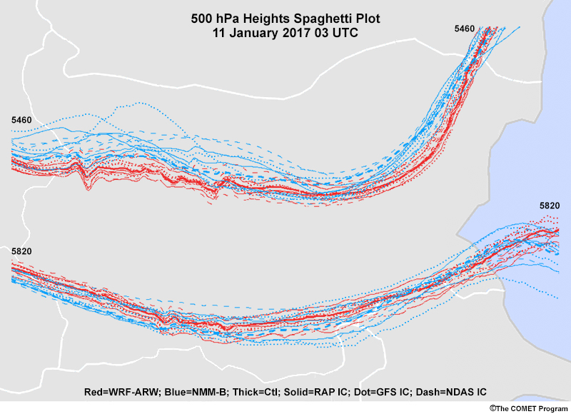
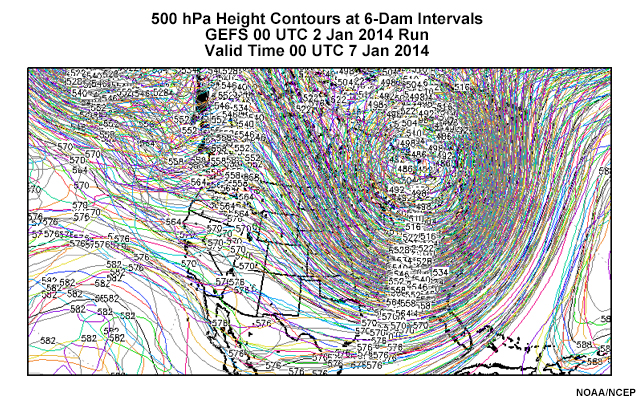
Spaghetti maps are plan-view maps of single values for a variable of interest from all of the ensemble members. They are typically plotted for one or a few key contour values (two in the example above). This keeps the presentation relatively simple while still giving a sense of the distribution of forecast outcomes for the areas around those contours. Contrast that plot with the one below, which contains all contours of the variable from all ensemble members. Clearly the result is hard to interpret!
Spaghetti maps can be generated for a variety of features, such as geopotential heights, precipitation of a certain amount, or a certain contour of temperature.
Interpretation
Spaghetti maps show the full distribution of members spatially. But you can also estimate differences in the timing and magnitude of weather features by examining the spatial arrangement of the members.
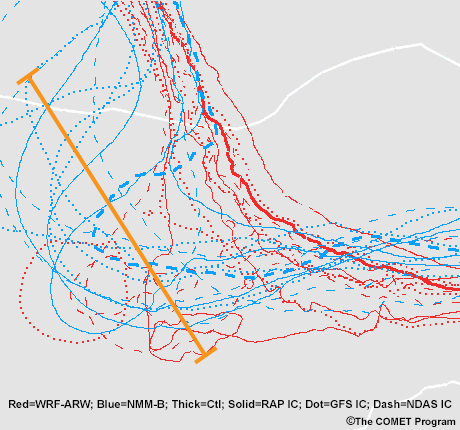
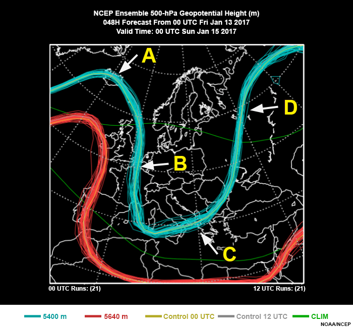
The map below shows the 5460 m contour members for 500 hPa. The members have significant spatial differences, as indicated by the orange bracket. What causes the difference? Clearly, some members show a strong trough while others place the axis significantly eastward. Some of this difference can be attributed to differences in timing, with some members bringing the system through earlier than others. But differences in the track of the low/trough may also be at play. Consulting a mean and spread map can help you determine the cause of these differences.
The solutions in this example also show great differences in magnitude. In the graphic below, the orange bracket encompasses solutions that develop a strong trough and even one that develops into a cutoff low. The green bracket shows members with much weaker troughing.
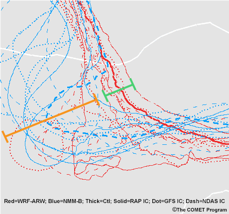
This example also highlights how clustering can be seen. The green bracket has an obvious cluster of similar solutions while the orange bracket shows a cluster with more- developed troughs.
The distance between members shows the amount of spread in the distribution at that location or time.
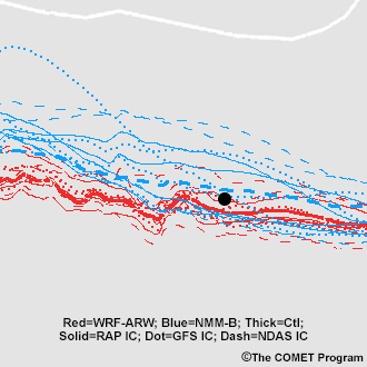
Additionally, you can use spaghetti maps to determine the probability of a threshold being met or exceeded. Simply count the individual members in a certain direction from a location of interest. The example below has 24 members, with 8 to the north of the area marked by the black dot. This means that there’s a 33% chance that the 500 hPa 5460 m height line is to the north of that location.
Outliers are obvious by being distinctly outside the rest of the range of possibilities.
Finally, it is easier to estimate whether a distribution is normal, multimodal, or skewed on spaghetti maps than other types of maps since all members are visible at one time. When members are normally distributed, you can estimate the most likely outcome by looking at the median or mean contour. This may often be indicated in bold black or another distinct colour.
Strengths & Weaknesses
Strengths:
- The full distribution of ensemble members can be viewed for specific contours, letting you estimate the shape of the distribution, presence of clustering, and most likely outcomes (mean or median if it is plotted).
- The distance between members provides an estimate of the spread and thus the EPS uncertainty.
- It is easy to estimate differences in feature magnitude.
- You can see where errors grow from in a time series (where the contours begin to grow apart).
Weaknesses:
- The maps can be difficult to read due to the high density of ensemble members around a forecast location.
- Since they typically show one or several contours, you do not get a full view of the entire member distribution.
- Determining whether feature location or timing differences are contributing to uncertainty can sometimes be difficult since both are often present at the same time.
Effective Use
Spaghetti maps are useful for looking at all member solutions to estimate the shape of the distribution, general spread, and differences in feature magnitude. They are best combined with other maps in the following ways.
- Use mean and spread plan-view maps to determine differences in feature timing versus location. They generalize all contours into mean contours with colour-shading of the spread, giving a fuller picture of uncertainty. It’s best to consult a mean and spread map before examining a spaghetti plot so you can choose an appropriate spaghetti contour or level to examine. Since we tend to be most interested in the probability of a forecast variable in regions in high uncertainty, it makes sense to examine spaghetti maps for contours that cross the regions of maximum spread.
- Use probability of exceedance/occurrence plan-view maps to estimate whether a threshold will be exceeded. That’s much easier than counting the members in a spaghetti plot!
Keep the following points in mind when using spaghetti maps.
- They can be used effectively at all time scales although they become more chaotic and difficult to read with increasing forecast time.
- Do not pick a single ensemble member as your “model of the day” since it may be best at that time but not as good in other times.
- Be careful when investigating closed circulations and contorted contour shapes since there can be multiple contours of the same value. This makes it difficult to identify the side on which the contour values are increasing or decreasing.
Examples, Part 1
Question
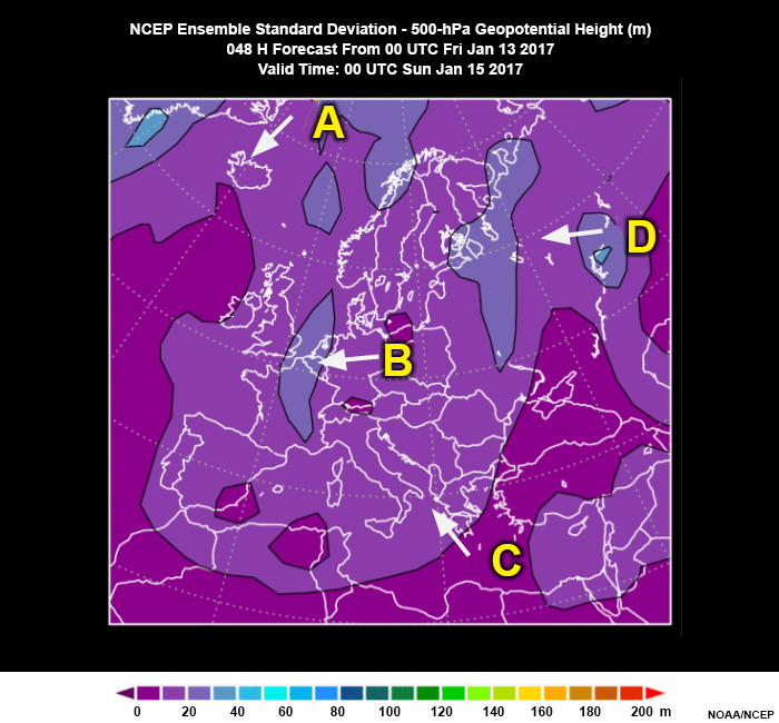
The spread is largest at point B even though the range is larger at point C. The spread is determined by how spread out ALL of the members are. Those farther away from a consistent core of members will show a smaller spread but can show a larger range.
Examples, Part 2
Question
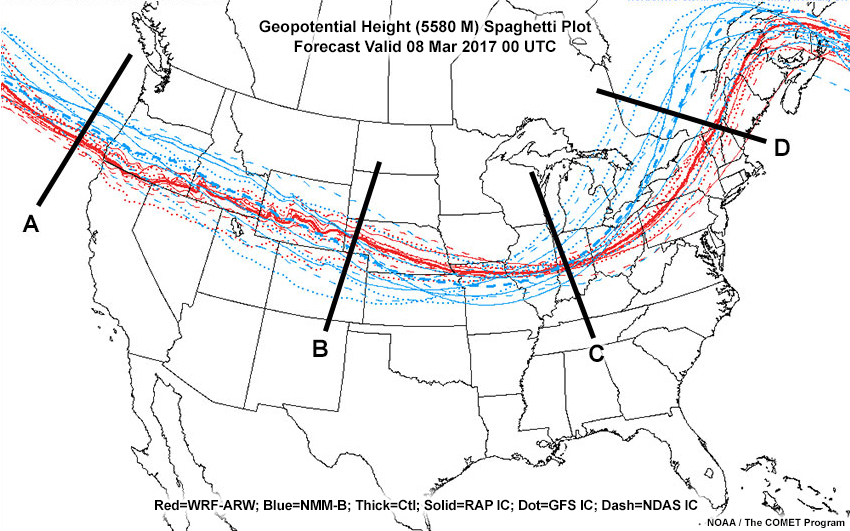
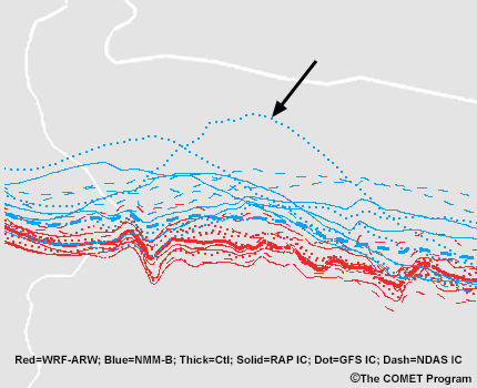
Based on this spaghetti plot, at which transverse line is there clustering of members?
The correct answer is d.
At line D, there are two clusters: one with a westward shift of the western portion of the ridge and the other with a more eastward shift. Although it may not look like it, these clusters are grouped by the two different dynamical physics cores since some of the light blue lines are also within the eastern cluster.
Links
- NCEP Spaghetti Plots for GEFS days 1 - 16: http://mag.ncep.noaa.gov/model-guidance-model-parameter.php?group=Model%20Guidance&model=gefs-spag&area=namer
- ESRL Spaghetti Plots GEFS days 1 - 15: https://www.esrl.noaa.gov/psd/map/images/ens/ens.html
- NCEP Spaghetti Plots days 3 - 14: http://www.cpc.ncep.noaa.gov/products/predictions/threats/briefs/hgtP1.html
- MSC Spaghetti plots days 1 - 15: http://weather.gc.ca/ensemble/index_e.html#spagat