Introduction
The National Weather Service (NWS) National Blend of global Models (NBM) is designed to serve as a starting point for creating U.S. national weather forecasts, based on the best possible science. For an overview of the NBM, see the lesson Introduction to the NWS National Blend of Global Models.
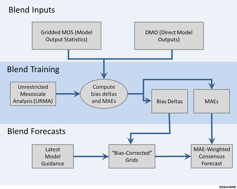
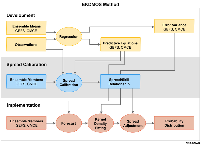
The NBM (or the Blend) is based on output from global models/ensembles, and statistically post-processed guidance. Below is a schematic of how the NBM temperature-based elements are derived. Details on the blending methodologies for various weather elements will be provided in a future lesson. In this lesson, we discuss the two main sources of information integrated into the Blend: Direct Model Output (DMO) and gridded Model Output Statistics (MOS).
Direct Model Output
NBM Version 2.0 (v2) focuses on using global deterministic and ensemble models for medium-range weather forecasting (day 3 through day 11). A deterministic model provides a single output forecast, while an ensemble provides a range of forecast outcomes from multiple model runs.
The following Direct Model Output (DMO) sources are integrated into the weather elements for NBM v2:
- Deterministic Global Forecast System (GFS), bias-corrected
- Global Ensemble Forecast System (GEFS), bias-corrected
- Canadian Meteorological Centre Ensemble (CMCE), bias-corrected
- North American Mesoscale Model (NAM), bias-corrected
- NAM-nests, bias corrected
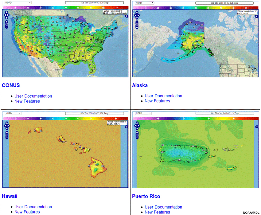
Example of temperature forecasts for several domains from the NDFD.
Direct Model Output (DMO) » Blend Weather Elements
Initially, the NBM will be produced for two forecast cycles per day (0000 and 1200 UTC) over the conterminous U.S. (CONUS) based on blending model guidance. The table below summarizes the weather elements and models used to produce the Blend.
Element |
URMA1 |
GDAS2 |
GFS |
GEFS Mean |
GEFS Members |
CMC |
CMCE Mean |
CMCE Members |
GMOS3 |
EKDMOS Mean |
NAM |
NAM Nest |
2-m Tmax |
CAHP |
CAHP |
CAHP |
CAHP |
CAH |
CAHP |
||||||
2-m Tmin |
CAHP |
CAHP |
CAHP |
CAHP |
CAH |
CAHP |
||||||
2-m T |
CAHP |
CAHP |
CAHP |
CAHP |
CAH |
CAHP |
CAHP |
CAHP |
||||
2-m Td |
CAHP |
CAHP |
CAHP |
CAHP |
CAH |
CAHP |
CAHP |
CAHP |
||||
10-m Wind Speed |
CAHP |
O |
CAHPO |
CAHPO |
O |
O |
O |
CAH |
CAHP |
CAHP |
||
10-m Wind Direction |
O |
CAHPO |
O |
|||||||||
10-m Wind Gust |
*CONUS, Alaska, Hawaii and Puerto Rico wind gusts are derived from NBM wind speed using Tattelman's equation. NBM wind gusts over the Great Lakes, GSL, Lake Okeechobee and ocean points are a blend of GFS, GMOS, NAM and NAM Nest |
|||||||||||
Sky Cover |
C |
CAHP |
CAHP |
CAHP |
CAH |
CAHP |
CAHP |
|||||
PoP12 |
C |
C |
C |
C |
C |
|||||||
QPF |
C |
C |
C |
C |
C |
|||||||
Relative Humidity |
*CONUS, Alaska, Hawaii and Puerto Rico derived from NBM 2-m temperature and dewpoint |
|||||||||||
Apparent T |
*CONUS, Alaska, Hawaii and Puerto Rico derived from NBM 2-m temperature, dewpoint and wind speed |
|||||||||||
Domain: C = CONUS, A = Alaska, H = Hawaii, P = Puerto Rico, O = Oceanic
1MAEs relative to URMA are used to weight winds and sky cover; temperature elements are bias-corrected and weighted relative to URMA
2GDAS is used to bias-correct oceanic winds
3GMOS is the gridded GFS MOS
Direct Model Output (DMO) » Global Forecast System
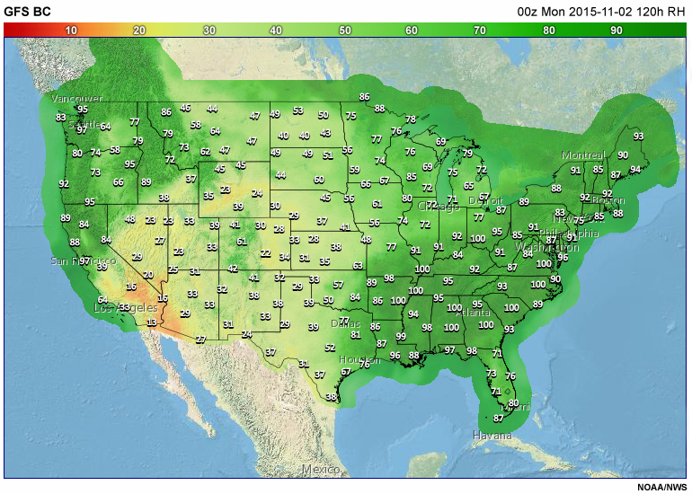
Example of a bias-corrected GFS relative humidity forecast.
The Global Forecast System (GFS) is a global spectral model that provides deterministic weather forecasts. It is run four times per day, out to 16 days. The resolution is equivalent to a grid spacing of ~10 km at midlatitudes up to 10 days. After 10 days, the GFS has a lower resolution. An Ensemble Kalman Filter (EnKF) uses 80-members to provide the flow-dependent error for the GFS hybrid 4-Dimensional Ensemble Variational (Hybrid 4DEnVar) system. This is used to obtain the initial conditions. For more information, see the Operational Models Encyclopedia's GFS page.
Question
Based on what you already know about global spectral models, what are they best at forecasting? Select all that apply.
The correct answers are b and d.
Global spectral models are best for forecasting the planetary wave pattern for the next seven days and QPF for the next five days. This is because spectral formulations allow for real-time integration of the fundamental equations over a longer time range than gridpoint models. Also, spectral models have global domains that are best for depicting planetary-scale features.
Direct Model Output (DMO) » Global Ensemble Forecast System
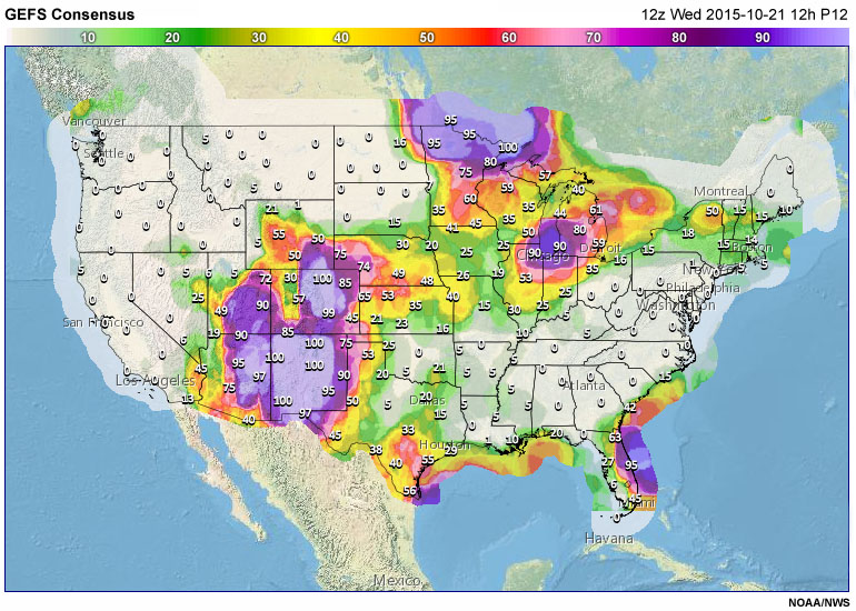
Percent of GEFS members producing measurable precipitation (0.01 inch or more).
The Global Ensemble Forecast System (GEFS) is a global spectral model made up of 21 ensemble members designed to quantify forecast uncertainty. It is run four times per day, out to 16 days. The resolution is equivalent to a grid spacing of ~35 km at midlatitudes up to 8 days. After 8 days, the GEFS has a lower resolution. The same physical parameterizations are used for each member in the GEFS (Zhu et al. 2007). To account for uncertainties in the physical processes, time tendencies for wind, moisture, and temperature resulting from model physics are randomly perturbed periodically. For more information, see the Operational Models Encyclopedia's GEFS page or the GEFS webcast.
Direct Model Output (DMO) » Canadian Met Centre Global Ensemble Prediction System
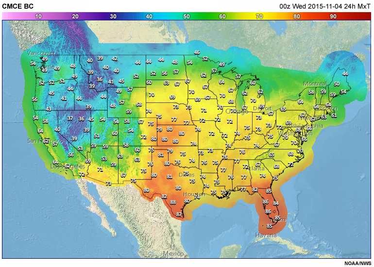
Example of a bias-corrected CMCE maximum temperature forecast.
The Canadian Meteorological Centre (CMC) Global Ensemble Prediction System (GEPS) uses a global gridpoint model to create 21 ensemble members from the CMC's Global Environmental Multiscale (GEM) model. The GEPS is run twice a day out to 16 days at a resolution of ~50 km at midlatitudes. Initial conditions are chosen from the 256-member ensemble used in the Canadian 4D-VAR data assimilation system. Each GEPS member uses unique physical parameterizations and perturbed observations. Time tendencies for wind, moisture, and temperature are randomly perturbed to account for model uncertainties. For more information, see the Operational Models Encyclopedia's GEPS page and links therein.
The NBM uses the ensemble mean from both the GEFS and GEPS.
Question
How does the inclusion of two ensemble mean forecasts benefit the Blend? Select all that apply.
The correct answers are a and c.
Bulk verification statistics suggest that the ensemble mean outperforms deterministic models over long periods of time. Deterministic models are more likely to capture individual unusual events with more accuracy than the means, but over time the means minimize error and reduce the potential for “big busts” when there is significant disagreement in the ensemble envelopes.
Direct Model Output (DMO) » North American Mesoscale Model
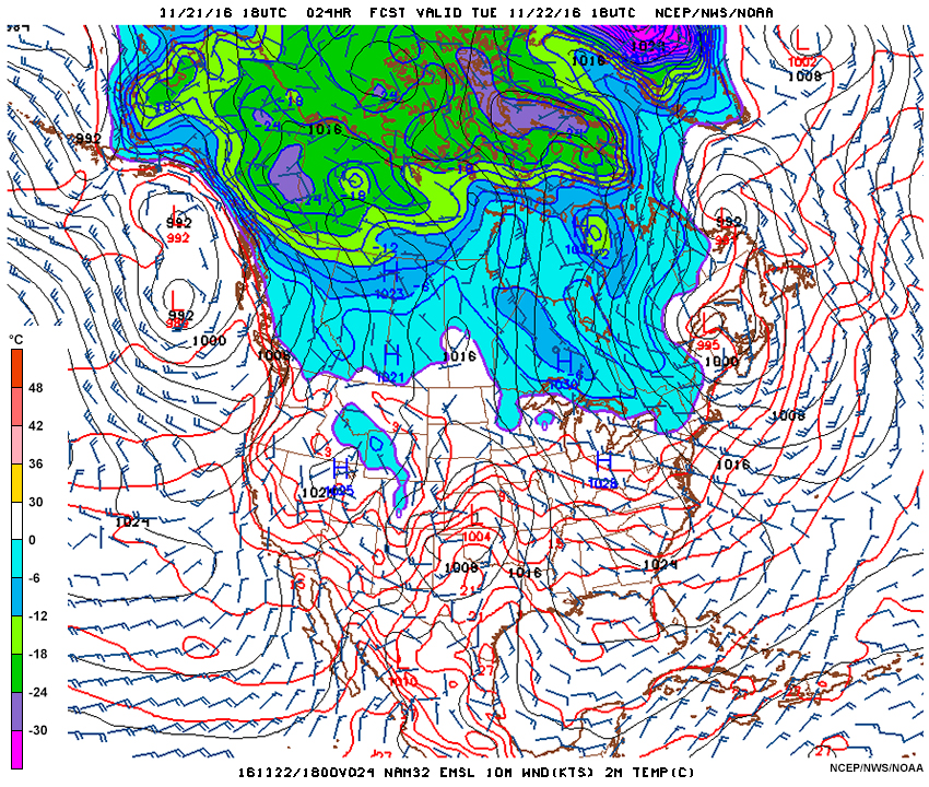
Example of a 10-m wind forecast from the 32 km NAM.
The North American Mesoscale Model (NAM) is a regional gridded model that provides deterministic weather forecasts. It is run four times per day, out to 84 hours. NAM has 12 km grid spacing, and uses the deterministic GFS boundary conditions on the edges of its domain. The NAM uses the Ensemble Kalman Filter as part of its 3DVar data assimilation system.
Direct Model Output (DMO) » North American Mesoscale Model Nests
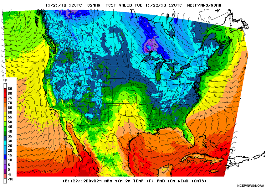
Example of a 2-m temperature and 10-m wind forecast from the 4 km NAM.
The CONUS nest run inside of the NAM domain is run at 4 km resolution. It provides deterministic forecasts, and is run in tandem with the parent NAM model out to 60 hours. Initial conditions are interpolated from the parent NAM, from which the NAM Nest is "spun up".
Model Output Statistics
Model Output Statistics (MOS) is a post-processing technique used for the Blend. MOS develops statistical relationships between observed weather elements (or predictands) at an individual station and appropriate variables (or predictors). The predictors can be obtained from model forecasts, past surface observations, or climatic information such as mean temperatures or precipitation. For rare weather elements (e.g. thunderstorms), stations with similar climatologies are grouped together to obtain these statistical relationships.
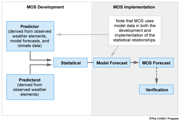
Flowchart of how Model Output Statistics are developed and implemented.
MOS is used frequently in the NWS to objectively interpret and "add value" to model output. Because MOS uses model output in the development and implementation of the statistical relationships, time lags can be incorporated into the relationships and certain systematic model errors can be accounted for. Weather models only approximate the physical processes that occur within the lowest layers of the atmosphere. Along with coarse resolution, surface weather forecasts are subject to biases and errors that tend to grow with time. Some of this bias is removed by MOS.
MOS predicts what models cannot predict well (e.g., 2-m temperature where the model elevation is not representative of a station). It can produce site-specific forecasts from a model that has insufficient resolution. Consequently, MOS can be thought of as an interpolation technique. MOS also assists forecasters by giving a built-in "first guess" for expected local conditions, and a model climatological memory for those unfamiliar with the model's behavior at a given weather forecast office (WFO).
Question
Based on what you have learned about MOS, how does adding MOS benefit the Blend? Select all that apply.
The correct answers are a and b.
The GEFS and CMCE have coarse resolution, ~35 km versus the 2.5 km National Digital Forecast Database (NDFD) grids. Therefore, MOS techniques can improve ensemble resolution using statistical post-processing.
Model Output Statistics » Data Sources
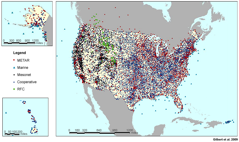
MOS stations for daytime maximum and nighttime minimum temperatures in the GFS MOS system.
MOS data are produced to match the elements and spatial/temporal resolution of the NDFD. Forecast models and MOS methodologies are used to develop sensible weather values for each MOS station within various networks (see map legend above).
Model Output Statistics » Statistical Method
The statistical method used for MOS is a multiple linear regression with forward selection. Multiple linear regression applies a linear regression using multiple predictors and a single predictand, in a series of steps known as forward stepwise selection.
Linear regression determines the relationship between the predictand and predictor(s) that fits the data in a way that minimizes errors. Below is a scatterplot of predictands vs. predictors and the line that best represents the relationship between the variables.
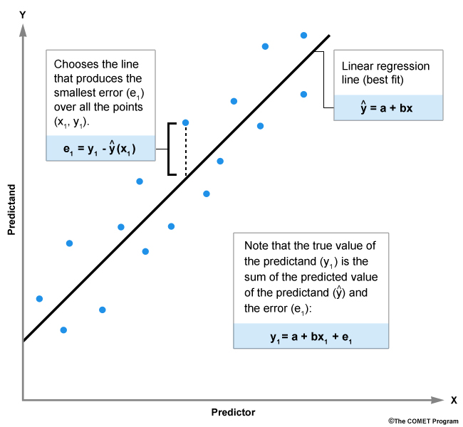
Diagram of the relationship between the predictand and predictor(s) for a linear regression.
The forward selecting multiple linear regression is iterative. First, potential predictors are selected using a simple linear regression. From a list of predictors that are relevant to the predictand data, a best predictor (i.e., the one with the best fit) is determined. A second set of comparisons is made using forward selection for the remaining relevant predictors. Each predictor is examined with respect to both the optimal predictor and the predictand, producing additional relationships. This process continues until the residual error is minimized using as many additional predictors as is necessary. The final group of predictors from the model output are those that best explain the predictands, or weather elements.
Model Output Statistics » Advantages and Limitations
Advantages
Since historical model data is used in its development, MOS can:
- account for systematic model errors and deteriorating accuracy at longer lead times
- account for the predictability of model variables by selecting those providing useful forecast information
- for example: using 850-hPa temperature forecasts as opposed to 2-m temperature forecasts to generate surface temperature guidance, in situations where the 850-hPa temperature is more accurately forecasted.
- interpolate the models to obtain point forecasts of weather elements
- produce more accurate guidance since multiple predictors fit the predictand data better
Limitations
The performance of MOS degrades for extreme events and at longer lead times. Model changes may alter the predictor/predictand relationships, and retrospective model forecast runs may not be long enough to obtain solid predictor/predictand relationships. Extreme events are often not well-represented in these cases. Furthermore, MOS equations are not flow regime dependent and differing flow regimes are combined to make the equations. Undersampling of any particular regime will result in problems when that regime is present.
Question
What advantages does MOS guidance bring to the Blend? Select all that apply.
The correct answers are a and c.
These factors affect all MOS used in the Blend. The effect of systematic model errors is reduced using MOS guidance, while the numbers of predictors is also reduced to those that produce the best relationship with respect to the predictand.
Model Output Statistics » MOS Used in the Blend
The MOS components in the NBM v2 include:
- Ensemble Kernel Density Model Output Statistics, bias-corrected (EKDMOS BC)
- GFS-based Gridded Model Output Statistics, bias-corrected (GMOS BC)
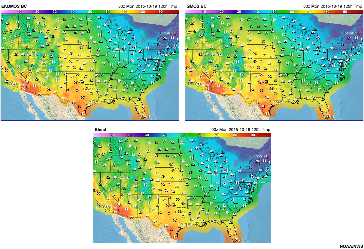
Example of temperature forecasts from the EKDMOS, GMOS, and the Blend. GMOS is the gridded GFS MOS.
EKDMOS
Ensemble models predict a range of possible forecast scenarios and help operational forecasters assess forecast uncertainty. The CMCE and GEFS members combined are known as the North American Ensemble Forecast System (NAEFS). The 21-member ensemble mean from both the GEFS and CMCE is ‘blended’ in the NBM v2. Ensemble Kernel Density MOS (EKDMOS) is a statistical post-processing technique that calibrates probabilistic forecast guidance for NAEFS. NAEFS contains errors and biases in its near-surface weather elements.
EKDMOS » Methodology
The graph below shows probability distributions of predicted and observed temperature values. Notice that the predicted (ensemble) spread is smaller than the observed spread. That is, the verifying observation frequently falls outside the range predicted by the ensemble members. The EKDMOS technique calibrates NAEFS forecasts by adjusting ensemble spread to produce statistically reliable probability distributions of weather elements.
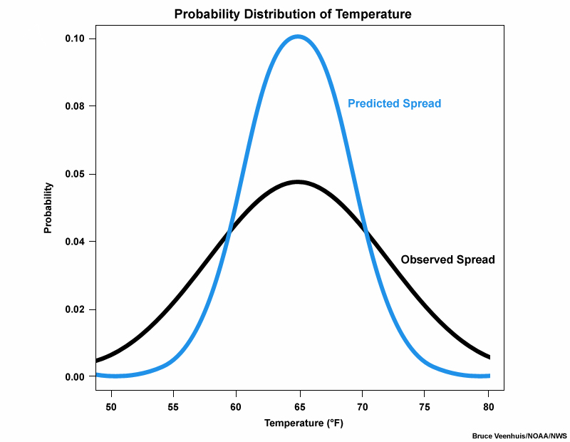
Comparison between predicted (ensemble) and observed spread in temperatures.
EKDMOS develops separate sets of MOS equations for the GEFS and CMCE using forward screening multiple linear regression and ensemble mean-based predictors. The MOS equations are applied to the NAEFS ensemble members to produce a set of 42 ensemble MOS forecasts for every projection, station, cycle, and element. These 42 forecasts are combined into an initial probability density function (PDF), then a second regression creates a ‘spread-skill’ equation. This ‘spread-skill’ equation takes the spread of the 42 ensemble MOS forecasts and predicts the expected accuracy of the ensemble mean MOS forecast.
The EKDMOS forecasts are analyzed onto 2.5-km grids for the CONUS using the Bergthorsson–Cressman–Doos-Glahn (BCDG) technique, as described in the next section on gridded MOS. For more information, see the NOAA NWS Meteorological Development Lab EKDMOS page.
Question
What is the order to transform NAEFS output onto gridded space? Click and drag each method into its correct order.
The correct sequence to transform the NAEFS output onto gridded space is:
- Multiple linear regression
- Spread adjustment
- Gridding
Gridded Model Output Statistics
The gridded MOS technique is used to interpolate MOS onto a 2.5-km grid for the Blend. The gridded GFS output (hereafter, GMOS) is part of the National Digital Guidance Database (NDGD). Gridded MOS was developed to provide forecasters guidance using high-resolution grids to match the elements and temporal/spatial resolution of the NDFD. Gridded MOS maintains the accuracy and skill of the original station-based MOS. In basic terms, gridded MOS is an objective analysis technique that interpolates station-based model output onto a high-resolution grid.
Gridded MOS was developed to produce forecast guidance:
- for the NDFD at a 2.5-km grid resolution
- with sufficient detail for forecast initialization
- with a level of accuracy comparable to station-based MOS
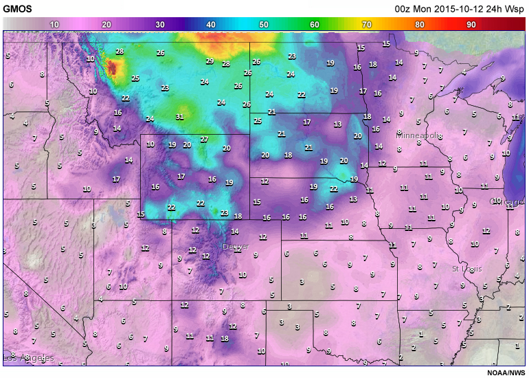
Example of a gridded GFS MOS (GMOS) wind speed forecast.
Gridded Model Output Statistics » Methodologies
Two methods are used to produce gridded MOS. The first is an objective technique of successive corrections to analyze station-based MOS forecasts to points, known as the BCDG analysis technique. This technique grids irregularly spaced station guidance to a regular grid. It develops regression equations at single-station sites, like traditional MOS. A constant is used as a first guess, before four iterative corrections are made using a distance-based weighted average, and the result is interpolated to a grid. The radius of influence varies and decreases with each iteration, to increase detail. A contour-following smoother is also used where there is little change in elevation. Land and water forecast points are differentiated and vertical corrections are made to all elements, except for probability of precipitation and wind direction. This is the most common method used to grid the weather elements.
The second method uses larger domains with similar climatology and applies the MOS approach to obtain a single equation set for a weather element over the entire domain. The equation is applied at grid points, and directly makes forecasts at each point. This method is used for various weather elements in the Blend during rare events (e.g. precipitation types, thunderstorms).
Numerous quality control checks are made to ensure consistency between and within elements. For more information, see the NOAA NWS Meteorological Development Lab gridded GFS MOS page.
Gridded Model Output Statistics » Advantages and Limitations
Gridded MOS has several strengths, one being a lack of discontinuities between WFO boundaries, evident in some forecast fields in the NDFD. Using vertical elevation differences to adjust some gridded MOS fields results in realistic features, which correspond well to the influencing terrain.
Deficiencies of gridded MOS include potentially large errors when strong surface-based inversions and rare events occur, as well as inconsistencies between gridded MOS grids and the station-based MOS they are based on.
Question
For each of the following situations, select whether the GMOS temperature forecast going into the Blend will perform well or poorly based on its advantages and limitations. Use the selection box to choose the answer.
The correct answers are displayed above. For the first situation, the GMOS temperature forecast should perform well because there should be good sampling of clear summer days for MOS development, and the lack of inversion would remove another challenge to the MOS forecast. The second situation is a rare event that would result in a poor MOS temperature forecast, while the third situation presents a strong temperature inversion adversely affecting MOS. The final situation should be well-handled by gridded MOS as there should be no temperature inversions and gridded MOS is designed to handle rugged terrain.
Coming Soon: Versions 2.1, 3.0, and 4.0
Two upgrades to the NBM will take place during 2017. The first upgrade, to version 2.1, will occur in winter 2017, with guidance added for 12-hour probability of precipitation (PoP12) and 6-hour quantitative precipitation (QPF06).
A more comprehensive upgrade will occur during summer 2017, when NBM version 3.0 is made operational. Expected changes include:
-
Increased run frequency from twice per day to hourly, using the latest available model runs
-
Development of a Short-Term Blend with hourly resolution to 36 hours, with an Extended Blend from 30 to 264 hours; 3-hourly through 192 hours and 6-hourly thereafter.
-
Addition of mesoscale models to the Short-Term Blend including HRRR, RAP, SREF, HiResARW, HiResNMM, and Global LAMP. The Navy Global Environmental Model (NAVGEM) may be considered for the Extended Blend.
- The Short-Term Blend will be updated on the SBN every hour requested, and the Extended Blend will be updated on the SBM four times per day.
NBM Version 3.0 will include the following new or updated products for the CONUS:
-
QPF01 and PoP01 (to 36 hours) to support Enhanced Short-Term Forecasts
-
Ceiling height/cloud base
-
Visibility
-
Blended inputs to support Weather type, Snow Amount, Ice Accumulation
-
Blended wind direction
-
Elimination of nearshore clipping; expand domain over oceans to support NWPS
-
Mitigation of high bias on PoP12 forecasts implemented in NBM v2.1.
Off-CONUS, until there is a verification data set available for PoP and QPF, PoP12 and 12-hour QPF (QPF12) will be determined using an alternative technique. Blended wind direction will also be made available.
Finally, NBM Version 4.0 will bring in more models and the initiation of probabilistic grids derived from calibrated component ensembles. Fields for 1-hour QPF (for National Water Model), probabilistic wind direction and speed, and probabilistic maximum and minimum temperatures will be added. Probabilistic grids will likely be made for the 5th, 10th, 25th, 50th, 75th, 90th and 95th percentile values.
Summary
The tables below summarizes Version 2.0 of the Blend, and the model products ingested into the Blend.
NBM System Attributes
System Name |
Areal Coverage |
Horizontal Resolution |
Cycle Frequency |
Forecast-Hour Frequency and Length |
NBM - CONUS (v2) |
CONUS NDFD expanded domain |
2.5 km |
2/day |
See table below by variable |
NBM Grid Durations |
Version 1.0 |
Version 2.0 |
Temperature |
3-h to 192 |
3-h to 192, 6-h to 264 |
Dewpoint |
3-h to 192 |
3-h to 192, 6-h to 264 |
Maximum Temperature |
24-h to 192 |
24-h to 258/270 |
Minimum Temperature |
24-h to 192 |
24-h to 258/270 |
Wind Speed |
3-h to 192 |
3-h to 192, 6-h to 264 |
Wind Direction |
3-h to 192 |
3-h to 192, 6-h to 264 |
Wind Gust |
3-h to 192 |
3-h to 192, 6-h to 264 |
Sky Cover |
3-h to 192 |
3-h to 192, 6-h to 264 |
Apparent Temperature |
3-h to 192 |
3-h to 192, 6-h to 264 |
Relative Humidity |
3-h to 192 |
3-h to 192, 6-h to 264 |
QPF06 |
6-h to 180 |
|
PoP12 |
12-h to 240 |
System Data Assimilation or Initialization Technique
System |
Attributes |
GMOS |
Calibrated GFS, linear regression models |
EKDMOS |
Calibrated GEFS and GEPS, linear regression models |
GFS, GEFS, NAM, NAM CoNUS nest |
Bias-corrected GFS, GEFS, NAM, and NAM CONUS nest direct model inputs |
GEPS |
Bias-corrected, direct model inputs (GEM) |
RTMA/URMA |
Analysis from bias correction and verification, future calibration |
Main summary points include:
Model Output Statistics (MOS) is a technique used to objectively interpret model output and produce site-specific guidance in gridded format for the Blend. It statistically relates observed weather elements to appropriate variables obtained from:
- Numerical Weather Prediction model forecasts
- Past surface weather observations
- Climatic data information
GMOS, EKDMOS, and the direct model output from GFS, NAM, NAM nest, and the ensemble means of the GEFS and GEPS are bias-corrected to the URMA and downscaled, where necessary, to the resolution of the NBM grid. How these products are weighted and merged into the Blend for different weather elements will be described in a subsequent lesson. The NBM is disseminated on the Satellite Broadcast Network and provides the basis for forecasts from local weather offices.
References
Glahn, H. R., K. Gilbert, R. Cosgrove, D. P. Ruth, and K. Sheets, 2009: The gridding of MOS. Wea. Forecasting, 24, 520–529.
Glahn, H. R., M. R. Peroutka, J. Wiedenfeld, J. L. Wagner, G. Zylstra, B. Schuknecht, and B. Jackson, 2009: MOS uncertainty estimates in an ensemble framework. Mon. Wea. Rev., 137, 246–268.
Gilbert, K.K., B. Glahn, R.L., Cosgrove, K.L. Sheets and G.A. Wagner, 2009: Gridded model output statistics: Improving and expanding. Preprints, 23rd Conf. Weather Analysis Forecasting and 19th Conf. Numerical Prediction, Omaha, NE, Amer. Meteor. Soc.
Veenhuis, B. A., and J. L. Wagner, 2012: Second moment calibration and comparative verification of ensemble MOS forecasts. Preprints, 21st Conf. on Probability and Statistics in the Atmospheric Sciences, New Orleans, LA, Amer. Meteor. Soc. https://ams.confex.com/ams/92Annual/flvgateway.cgi/id/19514?recordingid=19514.
Veenhuis, B.A., 2013: Spread Calibration of Ensemble MOS Forecasts. Mon. Wea. Rev., 141, 2467–2482. doi: http://dx.doi.org/10.1175/MWR-D-12-00191.1
Zhu Y., R. Wobus, M. Wei, B. Cui, and Z. Toth, 2007: March 2007 NAEFS upgrade. http://www.emc.ncep.noaa.gov/gmb/ens/ens_imp_news.html.
Contributors
COMET Sponsors
MetEd and the COMET® Program are a part of the University Corporation for Atmospheric Research's (UCAR's) Community Programs (UCP) and are sponsored by NOAA's National Weather Service (NWS), with additional funding by:
- Bureau of Meteorology of Australia (BoM)
- Bureau of Reclamation, United States Department of the Interior
- European Organisation for the Exploitation of Meteorological Satellites (EUMETSAT)
- Meteorological Service of Canada (MSC)
- NOAA's National Environmental Satellite, Data and Information Service (NESDIS)
- NOAA's National Geodetic Survey (NGS)
- Naval Meteorology and Oceanography Command (NMOC)
- U.S. Army Corps of Engineers (USACE)
To learn more about us, please visit the COMET website.
Project Contributors
Program Manager
- Dr. Elizabeth Mulvihill Page — UCAR/COMET
NWP Projects Coordinator
- Amy Stevermer — UCAR/COMET
Project Leads/Science Focal Points
- Dr. Bill Bua — UCAR/COMET
- Dr. Paula Brown — CIRA/Colorado State University
Project Leads/Instructional Design
- Dr. Paula Brown — CIRA/Colorado State University
- Tsvetomir Ross-Lazarov — UCAR/COMET
- Vanessa Vincente — CIRA/Colorado State University
Project Scientists
- Dr. Paula Brown — CIRA/Colorado State University
- Vanessa Vincente — CIRA/Colorado State University
Principal Science Advisors
- Dr. David Myrick — National Weather Service (NWS) Meteorological Development Laboratory
- Kathryn Gilbert — National Weather Service (NWS) Weather Prediction Center
- John Wagner — National Weather Service (NWS) Meteorological Development Laboratory
- Dr. Bob Glahn — National Weather Service (NWS) Meteorological Development Laboratory
- Jeff Craven — National Weather Service (NWS) Central Region Scientific Services Division
- Bruce Veenhuis — National Weather Service (NWS) Meteorological Development Laboratory
- Michael Staudenmaier — National Weather Service (NWS) Western Region Headquarters
Graphics/Animations
- Steve Deyo — UCAR/COMET
- Sylvia Quesada — UCAR/COMET
Multimedia Authoring/Interface Design
- Gary Pacheco — UCAR/COMET
COMET Staff, Fall 2015
Director's Office
- Dr. Rich Jeffries, Director
- Dr. Greg Byrd, Deputy Director
- Lili Francklyn, Business Development Specialist
Business Administration
- Dr. Elizabeth Mulvihill Page, Group Manager
- Lorrie Alberta, Administrator
- Hildy Kane, Administrative Assistant
- Austin Ricks, Student Assistant
IT Services
- Tim Alberta, Group Manager
- Bob Bubon, Systems Administrator
- Dolores Kiessling, Software Engineer
- Joey Rener, Student Assistant
- Malte Winkler, Software Engineer
Instructional and Media Services
- Bruce Muller, Group Manager
- Dr. Alan Bol, Scientist/Instructional Designer
- Steve Deyo, Graphic and 3D Designer
- Lon Goldstein, Instructional Designer
- Bryan Guarente, Instructional Designer
- Lindsay Johnson, Student Assistant
- Dr. Vickie Johnson, Instructional Designer (Casual)
- Gary Pacheco, Web Designer and Developer
- Sylvia Quesada, Intern
- Sarah Ross-Lazarov, Instructional Designer (Casual)
- Tsvetomir Ross-Lazarov, Instructional Designer
- David Russi, Spanish Translations
- Andrea Smith, Meteorologist/Instructional Designer
- Marianne Weingroff, Instructional Designer
Science Group
- Wendy Schreiber-Abshire, Group Manager
- Dr. Paula Brown, Visiting Meteorologist, CIRA/Colorado State University
- Dr. William Bua, Meteorologist
- Dr. Frank Bub, Oceanographer (Casual)
- Lis Cohen, Meteorologist (Casual)
- Patrick Dills, Meteorologist
- Matthew Kelsch, Hydrometeorologist
- Dr. Elizabeth Mulvihill Page, Meteorologist
- Amy Stevermer, Meteorologist
- Vanessa Vincente, Visiting Meteorologist, CIRA/Colorado State University