Disturbances in Cold Air Masses

Development of Forcing Mechanisms

Sensible and Latent Heat

As a cold air mass moves over a water surface, there is a transfer of sensible heat from the water to the air; this decreases the low-level stability of the air mass. The cold air mass has a low wet-bulb potential temperature, and there is a rapid transfer of moisture into the colder air as it modifies through the input of sensible heat. Clouds usually form soon after the air begins its over-water trajectory, signifying the release of latent heat. This deep, concentrated convection is frequently associated with polar low development.

This figure is a plot of potential temperature against height through the boundary layer of a cold air mass moving over a warmer water surface.

• Above a near-surface super adiabatic layer, a dry adiabatic lapse rate exists through the well mixed sub-cloud layer
• In the moist cloud layer the lapse rate will be equal to or close to the moist adiabatic lapse rate
• The transition layer defines the region of exchange and entrainment between the dry, warmer stable inversion layer above and the moist, cooler convective cloud layer below
• 1000-2000 m is the typical base for the inversion layer

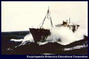
In a uniform flow, such as shown in this satellite image, there is little development other than a change in the structure of the cumulus cells. Mullen (1983) refers to Ellenton (1980) and Bosart (1981), who point out that surface heating is not directly responsible for cyclogenesis; instead it serves to establish a favourable low-level environment that likely facilitates development in response to later external forcing mechanisms

Baroclinic Instability

Baroclinic instability is associated with vertical shear of the mean flow. Baroclinic instabilities grow by converting potential energy associated with the mean horizontal temperature gradient (Holton 1992).

Enhanced low-level baroclinic zones can develop due to various conditions.

• Surface flows can become parallel or nearly parallel to the edge of pack ice, providing an opportunity for sharp baroclinic zones to develop
• The convergence of different low-level wind regimes and geographic features may also produce enhanced low-level baroclinic zones. This can lead to polar low development some considerable distance from the ice edge and the origin of the cold surface flow, as is shown in this example

The early view of polar lows was that they were the result of thermal instability. That changed when Harrold and Browning (1969) used radar to investigate a December 1967 polar low that crossed southwestern England. They found that much of the precipitation formed within uniformly ascending air, not by the merging of smaller-scale convective cells. In their study, the convection was confined to the rear of the system.

Rasmussen et al. (1994) state that polar low development as the result of purely baroclinic or convective process is rare. However, Rasmussen and Aakjær (1989) reported on two polar lows that affected Denmark and appeared to be baroclinic throughout their existence. One formed near the main frontal zone while the second formed in association with a cold vortex, which was the end product of an occlusion. In the earlier paper they state that such events are fairly common in the North Sea region.

Barotropic Instability

Barotropic instability is a wave instability associated with the horizontal shear in a jet-like current. Barotropic instabilities grow by extracting kinetic energy from the mean flow field (Holton 1992).

Barotropic instability can result in the formation of low-level shear vortices. Given further upper support, these vortices may then develop into polar lows. Rasmussen et al. (1994 and 1996) identify this as the likely development mechanism for the polar lows they studied in the Labrador Sea.

Cold Upper Troughs and Cold Lows

If a low-level baroclinic wave, barotropic shear vortices, or areas of enhanced convection have formed in a cold air mass, when will further development occur, if at all?

Rasmussen (1992) states, "In the case of a straight upper-level flow with little or small vorticity advection, polar lows will not develop even in cases when the upper-level temperatures are very low.” With this in mind we must look for forcing mechanisms. One obvious mechanism at northern latitudes is the cold upper trough and/or closed, cold-core upper vortex.

Rasmussen (1996) states that all of the polar lows he has investigated in the Labrador Sea were initiated by a cold upper trough or vortex. Furthermore, all of the cases investigated by Parker and Hudson (1991) and Parker (1992) involved a cold trough and/or closed vortex at the 500hPa level. In the Pacific, a comma cloud often accompanies the upper trough and can aid in early detection of a forcing mechanism.

A study by Noer et al. (2003) on the formation of polar lows in the Norwegian Sea area shows that in all cases a cold upper trough or vortex was associated with the low development. Indeed, it can often be shown that the movement and strength of this upper forcing can give good guidance on the subsequent evolution and motion of the system.

Conditional Instability of the Second Kind (CISK)

The similarity between some polar lows and tropical hurricanes has caused a number of researchers to speculate that like processes might be involved. Conditional instability of the second kind, or CISK, is one such process.

Charney and Eliassen (1964) defined CISK as a cooperative interaction between small-scale cumulus convection and a larger-scale disturbance where:

• The large-scale convergence organizes the cumulus convection
• Condensation heating in the clouds in turn supplies energy to the larger-scale system

CISK then implies a positive feedback mechanism at work in the system.

A number of researchers have in the past suggested that CISK is a driving force for polar lows. The feeling now appears to be that CISK may contribute to the development of polar lows, but is not the sole driving force.

Air-Sea Interaction Instability

Emanuel (1986) opposed the idea of CISK for tropical cyclones. He proposed that tropical cyclones result from air-sea interaction instability. Anomalous sea-surface fluxes of sensible and latent heat induced by strong surface winds and falling pressure lead to increased temperature anomalies and thereby to further increases in surface winds and pressure deficit.

Emanuel and Rotunno (1989) tested Emanuel's air-sea interaction theory for polar lows. Their case study used a simple non-linear analytical model and an axisymmetric numerical model. Results showed that the air-sea interaction hypothesis is consistent with observed arctic low development, but requires a pre-existing disturbance to act as a triggering mechanism before the air-sea interaction instability can operate.

References

Agee, Ernest M. and Steven R. Gilbert, 1989: An aircraft investigation of mesoscale convection over Lake Michigan during the 10 January 1984 cold air outbreak. J. Atmos. Sci., 46, No.13, 1877–1897.

Bader, M.J., G.S. Forbes, J.R. Grant, R.B.E. Lilley, and A.J. Waters, 1995: Images in Weather Forecasting. Cambridge University Press.

Charney, J. and A. Eliassen, 1964: On the growth of the hurricane depression. J. Atmos. Sci., 21, 68-75.

Emanuel, Kerry, A., 1986: A two stage air sea interaction theory for polar lows. Proc., The Third International Conference on Polar Lows, Norway.

Emanuel, Kerry A. and Richard Rotunno, 1989: Polar lows as arctic hurricanes. Tellus, 41A, 1-17.

Noer, G. and M. Ovhed, 2003: Forecasting of polar lows in the Norwegian and the Barents Sea. Proc. of the 9th meeting of the EGS Polar Lows Working Group, Cambridge, UK.

Harrold, T.W. and K.A. Browning, 1969: The polar low as a baroclinic disturbance. Quart. J. Roy. Meteor. Soc., 95, 710-723.

Holton, James, R., 1992: Introduction to Dynamic Meteorology. 3d ed. Academic Press Ltd., London, U.K..

Mullen, S., 1983: Explosive cyclogenesis associated with cyclones in polar air streams. Mon. Wea. Rev., 111, 1537-1553.

Parker, M.N. and Edward Hudson, 1991: Polar Low Handbook for Canadian Meteorologists. Environment Canada, Atmospheric Environment Service.

Parker, Neil, 1997: Cold Air Vortices and Polar Low Handbook for Canadian Meteorlogists. Environment Canada.

Parker, M.N, 1992: Polar lows in the Beaufort Sea and Davis Strait. Proc. Applications of New Forms of Satellite Data in Polar Low Research, Polar Low Workshop, Hvanneyri, Iceland.

Rasmussen, Erik A. and P.D. Aakjær, 1989: Two polar lows affecting Denmark. Vejret, Special Issue in English, The Danish Meteorological Society.

Rasmussen, Erik A., John Turner, and Paul Twitchell, 1992: Applications of new forms of satellite data in polar low research. Bull. Amer. Meteor. Soc., 74, 1057-1073.

Rasmussen, Erik A. and Anette Cederskov, 1994: Polar lows: A critical analysis. The life cycles of extratropical cyclones. Vol 111. Proc. of an International Symposium, Bergan, Norway.

Rasmussen, Erik A., Chantal Claud, and James F. Purdom, 1996: Labrador Sea polar lows. The Global Atmosphere and Ocean System, Vol. 4, 275-333.

Shapiro, M.A., T. Hampel, and L.S. Fedor, 1989: Research aircraft observations of an arctic front over the Barents Seas. Polar and Arctic Lows, Polar and Arctic Lows. Twitchell, P., E. Rasmussen, K. Davidson, Eds., A. Deepak Publishing.

Top of Page

Types of Disturbances

The Polar Low

Nordeng and Rasmussen (1992) called this particular polar low "A Most Beautiful Polar Low." It shows the classic features of a true polar low:

• The system is relatively small and non-frontal
• Cold air can be seen streaming southward west of the low
• A clear eye appears at the centre of the system. It is this clear area that helps give rise to the term “arctic hurricane” that is often seen in the literature; for example, in Emanuel and Rotunno (1989).
• The northern spiral arm separates cold air streaming off the ice surface from a modified cold air mass with open cellular convection

The European Polar Lows Working Group (EPLWG) published the following definition of a polar low at their June 1994 meeting in Paris:

"The term 'polar mesoscale cyclone' is the generic term for all meso-alpha (200 - 2000 km) and meso-beta (20 - 200 km) cyclonic vortices poleward of the main polar front. The term 'polar low' should be used for intense maritime polar mesoscale cyclones with scales up to 1000 km with a near surface wind exceeding 15 m/sec (30 knots)."

A more up-to-date definition by Rasmussen and Turner (2003) states:

"A polar low is a small, but fairly intense maritime cyclone that forms poleward of the main baroclinic zone (the polar front or other major baroclinic zone). The horizontal scale of the polar low is approximately between 200 and 1000 kilometres and surface winds near or above gale force."

Rasmussen (1994) suggested classifying polar lows into primary and secondary types. The primary type are those initiated as the result of a cold core vortex. Those associated with all other vortices that fit the definition of a polar low belong in the secondary category.

The majority of polar lows seen in Canadian waters fall into the primary category. However, there are some vortices in which baroclinic processes appear more important than convection during the mature phase, and these would fall into the secondary category. Some of the vortices forming along the ice edge of southern Davis Strait appear to fall in this secondary category.

European cases are often a result of pre-existing baroclinic effects and are therefore of the secondary category. Occlusions from mature synoptic-scale lows are a favoured mechanism between the British Isles and southern Greenland, while primary polar lows are generally confined to the area north of Iceland across to the Barents Sea.

Examples of Polar Lows

Here are two examples of polar lows in the Labrador Sea and the Gulf of Alaska.

The cloud pattern accompanying the Labrador Sea polar low is common for systems developing in the northwestern portions of the Labrador Sea. In their paper "Labrador Sea Polar Lows," Rasmussen et al. (1996) studied a number of Labrador Sea polar lows, all of which tended to form in the same general area and develop characteristic cloud patterns. The main features are the cloud bands northward and eastward from the centre. The eastward band or tail frequently marks a boundary between colder arctic air to the north and modified arctic air flowing eastward on the southern side of the system.

The Comma Cloud

The term "comma cloud" is used to describe a variety of comma-shaped cloud systems both over water and land. In this discussion it is used to describe comma-shaped cloud patterns poleward of the northernmost jet stream.

• with overlay
• hide overlay

Zick (1983) shows the typical relationship between a comma cloud and a major frontal cyclone. Here, the satellite imagery is of the northeast Pacific with the comma cloud positioned west of a main frontal zone that is visible over the Alaskan Panhandle, British Columbia, and Yukon

Mullen (1983) refers to an earlier report by Anderson (1969) in which he first pointed out that a cold air comma cloud is:

• Invariably downstream of an upper-tropospheric vorticity maximum
• In a region of 500-hPa vorticity advection
• Ahead of a shortwave trough or in the left exit region of a jet

Businger and Reed (1989) add that the comma cloud typically begins as a region of enhanced convection and geographically is most likely to be observed over the western oceans in areas where cold air is being advected over warmer water surfaces.

Reed (1979) makes the following comments about comma clouds:

• The dimensions of the comma-shaped cloud patterns are typically of the order of 1000 km in the direction normal to the southern front and 500 km in the parallel direction
• In cases of multiple systems, 1000-1500 km is a typical spacing
• A surface pressure trough lies under the trailing edge of the comma tail and, in the more intense cases, a surface low pressure center lies under the comma head
• Wave cyclones are initiated when the disturbances approach sufficiently close to the main frontal band
• The notch of the comma lies in the region of strong horizontal shear on the poleward side of the jet stream axis at 500 hPa
• The comma lies in a region of appreciable baroclinity, on the cold side of the baroclinic zone where the lapse rate is conditionally unstable through a considerable depth

The Instant Occlusion

If the distance between the comma cloud and frontal wave becomes small enough, the two features may combine with the resultant cloud closely resembling that of a mature occluded cyclone (Mullen, 1983). This time series over the Gulf of Alaska at 1845 UTC shows a comma cloud in the cold air mass north of the main frontal band. Nine hours later, at 0545 UTC, there is an indication of a weak wave developing on the main front. The comma cloud then proceeds to merge with the main front over the next 24 hours.

This process represents explosive cyclogenesis on a scale much larger than polar low vortices.

Reverse-Shear Flow

Vortices and polar lows are often observed to form in an area of reverse shear. Reverse shear refers to the situation in which the storm motion is in the opposite direction to the thermal wind. This is unlike the situation that prevails with the comma cloud type, which propagates in the direction of thermal wind (Businger and Reed, 1989). Duncan (1978) was the first to identify the reverse-shear case and showed that baroclinic development is favoured in regions of reversed shear.

In forward shear the colder air lies to the left of an observer positioned with his/her back to the wind. The thermal wind is positive and the actual wind increases with height. In a reverse-shear flow, warmer air lies to the left of an observer facing downwind. This produces a negative thermal wind, and the actual wind will decrease with height.

In both cases, the upward motion and comma-shaped cloud pattern are located where the thermal wind advects positive vorticity (i.e., down-shear of the trough). Because of the opposite relationships between thermal winds and steering winds, the cloud system lies ahead of the trough in the case of forward-shear and to its rear in the case of reverse-shear flow.

Reed and Duncan (1987) followed a series of disturbances that formed during a two-day period in January 1983. The disturbances were spaced about 500-600 km apart and moved southwestward at 10 knots. These lows were steered southwestward in conformity with the low-level winds. These winds were strongest near the surface where the thermal gradient was also strongest.

• 1000 hPa
• 850 hPa
• 700 hPa
• 500 hPa

From the orientation of the isotherms on the 1000-hPa and 850-hPa charts, it is apparent that the thermal wind is directed opposite to the low-level flow. Note that at these heights, the colder air lies to the right of an observer facing downwind, and the actual wind decreases with height.

Conditions for reverse-shear flow are not uncommon in the northern Labrador Sea and Davis Strait. When synoptic-scale lows pass south of Greenland they often develop a surface trough northward along the west Greenland coast. During the winter months this can produce a situation where the surface flow is closely oriented to the ice surface. This aids in the formation of a low-level baroclinic zone along the ice edge. Businger and Reed (1989) and Rasmussen (1994) state that these boundary-layer fronts, separating modified and unmodified air, appear to play a significant role in the development of baroclinic vortices. Although many remain weak circulations, others may develop into polar lows if they receive significant upper forcing.

A similar reverse-shear situation can be found at times north and east of Iceland. Here, arctic air flow at the surface is opposite to the direction of the thermal wind in the lower atmosphere. Any disturbance at the lower levels, including polar lows, tends to move slowly. If the pattern is persistent, then several shallow disturbances can develop over the course of a few days.

Shear Vortices and Lines of Enhanced Convection

A uniform flow of cold air is seldom sufficient and perhaps never sufficient by itself for development of true polar lows. Øakland (1989) says that for convection to be the energy source there must be spatial variations. The presence of a capping inversion is also necessary as it prevents deep convection from becoming widespread. The deep convection is then confined to or focused on the area immediately beneath the forcing mechanism.

This series of vortices over the Labrador Sea formed along a frontal zone. This frontal zone separates cold arctic air streaming southward behind a synoptic system southeast of Greenland from a warmer air mass that has moved around this low and lies in a surface trough extending from the low upward along the west Greenland coast.

This image shows cold air streaming across the Labrador Sea behind a major synoptic system that has moved east of Greenland. The change from shallow to deeper convection is obvious as the air moves further from the ice edge and the cloud pattern becomes open cellular. The flow appears fairly uniform. But an area of weak convergence and enhanced convection is evident downstream of the arrows. Interestingly, this area corresponds to the section of the Labrador Sea that experiences the highest frequency of polar low development. The cases by Rasmussen et al. (1996), Moore et al. (1996), and Mailhot et al. (1996) all formed in this general area.

Rasmussen et al. (1996) refer to a low-level jet that often develops because of the flow through Hudson Strait and extends over the Labrador Sea. This feature is often visible as streamers emanating from the adjoining capes. Small vortices are occasionally observed along the streamers.

Rasmussen (1996) also mentions the effect that the Torngat Mountains may play. Being a relatively high range, cold air over Labrador will have a tendency to flow around this feature. The flow south of the mountains is nearly westerly. The flow in the area to the north is northwesterly. The enhanced convection appears to be the result of this geographicaly induced convergence.

Vortices and Convergence Lines

Another area for the formation of vortices is along a boundary layer front formed due to the convergence of air streams with different over-water trajectories. For example, the eastward extending tail of the Labrador Sea polar low in this image lies along a frontal zone resulting from the convergence of two arctic air masses with different over-water trajectories.

Northern European cases are often preceded by the presence of convergence lines or isolated baroclinic zones that give rise to an organized pattern of convection. Vortices can sometimes be seen at the boundary between air from different origins. Usually, a line of bright cloud tops is observed, as in this example.

References

Anderson, R.K., J.P. Ashman, F. Bittner, G.R. Farr, E.W. Ferguson, V.J. Oliver, and A.H. Smith, 1969: Applications of meteorological satellite data in analysis and forecasting. ESSA Tech. Rep. NESC 51 [NTIS AD-697 033].

Bader, M.J., G.S. Forbes, J.R. Grant, R.B.E. Lilley. and A.J. Waters, 1995: Images in Weather Forecasting. Cambridge University Press.

Businger, S. and R. Reed, 1989: Cyclogenesis in cold air masses. Wea. Forecasting,
4. No. 2, 133-156.

Duncan, C.N., 1978: Baroclinic instability in a reversed shear flow. Meteor. Mag. 107, 17-23

Emanuel, Kerry A. and Richard Rotunno, 1989: Polar lows as arctic hurricanes. Tellus, 41A, 1-17.

Mailhot J., D. Hanley, B. Bilodeau, and O. Hertzman, 1996: A numerical case study of a polar low in the Labrador Sea. Tellus, 48A, 383-402.

Moore, G.W.K.., M.C. Reader, J. York, and S. Sathiyamoorthy, 1996: Polar lows in the Labrador Sea: A case study. Tellus, 48A, 17-40.

Mullen, S., 1983: Explosive cyclogenesis associated with cyclones in polar air streams. Mon. Wea. Rev., 111, 1537-1553.

Noer, G. and M. Ovhed, 2003: Forecasting of polar lows in the Norwegian and the Barents Sea. Proc. Ninth meeting of the EGS Polar Lows Working Group, Cambridge, UK.

Nordeng, Thor Erik and Erik A. Rasmussen, 1992: A most beautiful polar low: A case study of a polar low development in the Bear Island region. Tellus, 44A, 81-99.

Øakland, Hans, 1989: On the genesis of polar lows.Polar and Arctic Lows. Twitchell, P., E. Rasmussen, and K. Davidson, Eds., A. Deepak Publishing.

Parker, Neil, 1997: Cold Air Vortices and Polar Low Handbook for Canadian Meteorologists. Environment Canada.

Rasmussen, Erik A.and Anette Cederskov, 1994: Polar lows: A critical analysis. The Life Cycles of Extratropical Cyclones, Vol. 111. Proc. of an International Symposium, Bergan, Norway.

Rasmussen, Erik A., 1995: Polar Lows News - The Newsletter of the EGS Polar Lows Working Group. June 9, 1995, No. 5, Dr. G. Heinemann, Chairman.

Rasmussen, Erik A., Chantal Claud, and James F. Purdom, 1996: Labrador Sea Polar Lows. The Global Atmosphere and Ocean System, Vol. 4, 275-333.

Rasmussen, Erik A.and John Turner, 2003: Polar Lows: Mesoscale Weather Systems in the Polar Regions, Cambridge University Press.

Reed, R., 1979: Cyclogenesis in polar air streams. Mon. Wea. Rev., 107, 38-52.

Reed, R. and C. Duncan, 1987: Baroclinic instability as a mechanism for serial development of polar lows: A case study. Tellus, 39A, 376-384.

Zick, 1983: Method and results of an analysis of comma cloud developments by means of vorticity fields from upper tropospheric satellite wind data. Meteor. Rundsch. 36, 69-84.

Top of Page

Development of a Polar Low

Pre-development Conditions

There is usually a recognizable series of events leading to the development of a polar low. They are:

• A cold outbreak producing a flow of arctic air from an ice or land surface over a warmer water surface. This is often set up by the passage of a synoptic-scale cyclone. In a study by Wilhelmsen (1985) the average difference between the over-land and over-water temperatures was about 20°C.
• The formation of shallow baroclinic zones either along the ice edge or in the cold air stream. Away from the ice edge, these may be old occlusions or airflow boundaries forming arctic fronts.
• The formation of enhanced convection and/or low-level vortices in the cold air mass. These may be due to convergence or the existence of shallow baroclinic zones of low-level horizontal shear.
• The approach of an upper-level cold trough or closed vortex. This is usually observed at the 500 hPa level with temperatures below -35°C. Rasmussen (1994) gives a threshold value of
  -42°C. -30 to -35°C should raise caution, particularly in the early season, where the sea temperatures may be higher.
• The approach of a jet maximum or an area of PVA.
• The approach of a comma cloud. This is more apt to be seen in the northeastern Pacific and northeastern Atlantic.

Businger (1987) states that, "...once environmental conditions favourable for the formation of polar lows have developed they often persist and can result in several consecutive days on which polar lows occur."

Formation of the Mature Polar Low

Once the precursors have been identified, the challenge is to forecast the likely timing and position of a polar low. Where the low-level disturbance and upper-level forcing are forecast to coincide, this may be considered the most likely position for rapid development. Thus, an estimate of the position and timing of polar low formation may be made.

The transformation from a vortex to a polar low is usually very rapid. This is the result of both the dynamic forcing associated with the upper system and the initiation of deep convection resulting from decreased mid- and high-level stability. It is at this time that CISK (conditional instability of the second kind) and/or air-sea interaction instability may begin contributing to the deepening process. Surface winds will rapidly increase to gale force or stronger, thus meeting the adopted criterion for a true polar low. At times an eye will be visible on satellite imagery. Studies have shown that a warm core often forms (Rasmussen 1985, Shapiro et al. 1987).

On occasion, a polar low may develop hurricane force winds. This degree of deepening requires strong low-level convergence and or upper-level divergence. The resulting cloud pattern will become asymmetrical with an anticyclonically curved cirrus shield reflecting the outflow region (Fett et al. 1993).

Sidebar: Fett et al. (1993) reported on the passage of a polar low over St. Paul Island that produced a three-hour pressure drop of 13 hPA and a three-hour pressure rise of 13 hPa as it passed over the station. At the same time the temperature rose and fell 4°C.

TWeather and Sea State in a Mature Polar Low

By the time a polar low reaches a mature state, heavy snow showers and blowing snow will have developed and surface visibilities will frequently be reduced to near zero. Rapid changes in wind direction may occur due to the small size of the system. Lightning may be observed. Heavy in-cloud aircraft icing may also occur.

The small size of the polar low and the strong curvature might lead one to reach the conclusion that significant wave development would be fetch-limited. This is not always the case and presents additional risk to offshore activity. Fett et al. (1993) states that a St. Paul Island polar low produced 60-knot winds and 9-meter waves as measured by a Soviet icebreaker.

Intense circulations, such as tropical cyclones and polar lows, have the potential to develop large ocean waves. Usually in the case of a tropical cyclone, the larger, quicker-moving waves escape beyond the generation area, propagating ahead of the storm as decaying swell waves. However, as a tropical cyclone move to higher latitudes, the circulation is more likely to move at a velocity close to the group speed of the waves within the storm. In particular, waves to the right of the storm track usually propagate in the direction of the storm's motion, thereby allowing for prolonged forcing by the wind. The fetch becomes trapped within the storm as it moves along. Under ideal conditions, the significant wave height generated within the trapped fetch can grow to over twice the height of a wave associated with a stationary storm.

On the right side of the storm in relation to its movement, the winds will be at their strongest, while to the left the wind direction will oppose both the system itself and the broad-scale flow. For example, along the Norwegian coast the presence of a polar low close to the coast can induce offshore (easterly) winds to the north of its center. This has the effect of replacing an unstable, showery flow with clearer, more stable conditions.

Motion of Polar Lows

Because polar lows generally develop well behind synoptic systems, they are likely to have a moderate steering flow above them and thus may move faster than the initiating low (which may have slowed down or stalled). Speeds of 20 to 30 knots are not uncommon.

Because of their shallow nature, the steering flow will often be found at a lower level than that normally associated with synoptic systems. Businger and Reed (1989) suggest using the 850-700 hPa wind field. In the case of reverse shear lows, the steering flow may be quite light. A rule of thumb suggests that the actual speed of propagation is often 1/3 to 1/2 of the wind speed at the steering level (Noer et al. 2003).

Renfrew et al. (1996) examined three cases of multiple polar lows occurring in the Bear Island area. They noted that binary interaction between pairs of polar lows can cause a cyclonic co-rotation of the two lows when the lows were in the same vicinity.

Binary rotation is probably not surprising to many operational meteorologists who have observed upper-level vortices rotate, especially at northern latitudes.

Dissipation of Polar Lows

Polar lows making landfall or moving over an ice surface will rapidly weaken as their source of energy is cut off. If they stay over water, they may persist for several days. However, they are more likely to pass through the mature stage and begin to degrade into a larger convective vortex within a short time period.

Cold air vortices may also become involved with fronts or synoptic systems. Since they normally form deep within the cold air mass, this is more apt to be the fate of a dissipating vortex rather than a mature polar low.

A database compiled by Hanley and Richards (1991) was examined to determine the length of time vortices were followed on satellite imagery, keeping in mind that a number of factors may have resulted in the termination of the satellite archive for a particular vortex. The results show that the majority of cases were followed for less than 24 hours. This indicates, but does not confirm, a short duration for the systems observed in their study.

References

Bader, M.J., G.S. Forbes, J.R. Grant, R.B.E. Lilley, and A.J. Waters, 1995: Images in Weather Forecasting. Cambridge University Press.

Businger, S. and R. Reed, 1989: Cyclogenesis in cold air masses. Wea. Forecasting,
4. No 2., 133-156.

Dysthe, K.B. and A. Harbitz, 1987: Big waves from polar lows? Tellus, 39A, 500-508.

Fett, R.W., R.E. Englebretson, and D.C. Perryman, 1993: Forecasters Handbook for the Bering Sea, Aleutian Islands, and Gulf of Alaska. U.S. Naval Research Laboratory. NRL/PU/7541-93-0006.

Hanley, D. and W.G. Richards, 1991: Polar Lows in Atlantic Canadian Waters 1977-1989. Report: MAES 2-91. Scientific Services Division, Atlantic Region, Atmospheric Environment Service.

Noer, G. and M. Ovhed, 2003: Forecasting of polar lows in the Norwegian and the Barents Sea. Proc. Ninth meeting of the EGS Polar Lows Working Group, Cambridge, UK.

Parker, Neil, 1997: Cold Air Vortices and Polar Low Handbook for Canadian Meteorologists. Environment Canada

Rasmussen, Erik A., 1985: A case study of a polar low development over the Barents Sea. Tellus, 37A, 407-418.

Rasmussen, Erik A. and Anette Cederskov, 1994: Polar lows: A critical analysis. The life cycles of extratropical cyclones. Vol. 111. Proc. of an International Symposium, Bergan, Norway.

Renfrew, Ian, G.W.K. Moore, and Aashish A. Clerk, 1996: Binary interactions between polar lows. Submission to Tellus, 22 November 1996; also Extended Abstract, Workshop on Theoretical and Observational Studies of Polar Lows, St. Petersburg, Russian Federation, 23-26 September 1996.

Shapiro, M.A., L.S. Fedor, and Tamara Hampel, 1987: Research aircraft measurements of a polar low over the Norwegian Sea. Tellus, 39A, 272-306.

Wilhelmsen, K., 1985: Climatological study of gale-producing polar lows near Norway. Tellus, 37A, 451-459.

Top of Page

Climatology of Cold Air Vortices and Polar Lows

Reference Map and Seasonal Ice Coverage

Reference Map

Cold air vortices and polar lows occur in areas where cold air has an opportunity to flow over a water surface. Additionally, polar lows are most often associated with an upper-level cold core low or cold upper trough. This map shows areas susceptible to these conditions during parts of the year.

Seasonal Variations in Genesis Areas

'

Ice cover charts can be used to gain an insight on the geographic and seasonal variation of areas favourable for polar low development.

September represents the period of minimum ice cover. However, the availability of cold air places this month at the shoulder of the fall polar low season. It is the time of maximum open water in the Beaufort and Chukchi Seas as well as in Baffin Bay.

By early October the risk of polar low development in the Beaufort Sea is all but over, and by late December the risk of development in Hudson Bay and Baffin Bay has also passed. The southeastern portions of the Hudson Strait remain ice free most years. Ice cover eventually extends southward along the Labrador Coast to Newfoundland but the major portion of the Labrador Sea remains open and is a prime polar low development area.

The Gulf of Alaska also remains open year round and is a prime development area. Additionally, the occurrence of comma clouds is higher in the North Pacific than over Northern Atlantic waters (Carleton, 1985), which adds another dimension for the forecaster to consider.

The maximum extent of sea ice cover east of Greenland is limited to the northernmost areas of the region. To the east of Spitsbergen, the ice often stretches down to Bear Island, but this varies during the season according to the weather. In the easternmost part of the North Atlantic basin, the Kara Sea east of Novaya Zemlya is ice-covered from November on, but the Barents sea west of Novaya Zemlya stays ice free most of the winter. These areas together with the central Arctic ice sheet form the main sources of cold low-level air during the winter season.

The sea surface temperature in this region is strongly influenced by the Gulf current, which occupies the southern part of the Norwegian and the Barents sea. The Gulf current divides into two branches. One moves east along the north Norwegian coast, but weakens as it approaches Novaya Zemlya. The other branch moves north into the waters west of Spitsbergen. This makes for a steadily rising temperature from the ice edge in the north to the Norwegian coast in the south, giving prime conditions for convective activity to form in a northerly flow.

References

Carleton, Andrew, 1985: Satellite climatological aspect of the "polar low" and "instant occlusion". Tellus, 37A, 433-450.

Parker, Neil, 1997: Cold Air Vortices and Polar Low Handbook for Canadian Meteorologists. Environment Canada

Top of Page

Regional Climatology: Pacific and Canadian Waters

Pacific Climatology

A primary area of polar low development in the Pacific is the northern portion of the Gulf of Alaska. Businger (1987) recorded the geographic locations of spiral cloud signatures associated with polar lows in this region for the period 1975-1983. He found that once conditions favourable for polar low development are established, they often persist for several days, resulting in the formation of more than one polar low.

Closer observation of these statistics suggests that many of the vortices that develop in the Gulf of Alaska tend to drift southeastward, remaining off the mainland coast as they dissipate.

Yarnal and Henderson (1989) interpreted satellite imagery for seven five-month seasons between November and March, 1976/77-1983/84. They subjectively classified observed polar lows into two categories: comma cloud and spiral form. They then evaluated how many evolved to a higher stage of development.

Their results:

• Only six comma-cloud polar lows were detected in their database, of which three evolved to a high stage. Perhaps more noteworthy is the fact that relative to the western Pacific, few comma-cloud polar lows were observed over the eastern Pacific.
  
• The maximum number of spiral-form polar lows was observed in the northern Gulf of Alaska. But in the sample studied, none progressed beyond this form. For the forecaster this implies that at least with respect to the Gulf of Alaska, once a spiral-form polar low has formed, the risk of further development is minimal.

Pacific Climatology: Instant Occlusions

Instant occlusions are also significant events to consider. Mullen (1983) identified these as potential initiators of explosive cyclogenesis. Yarnal and Henderson (1989) state that "... although the eastern North Pacific is an area of low polar low frequency, the potential for explosive cyclogenesis is much greater in this part of the basin because of the concentration of instant occlusions. Thus, the entire extratropical west coast of North America is exposed to the dangers of these storms." Note that the reference here is to the eastern Pacific, and not the Gulf of Alaska where polar lows are more likely to be observed.

Northern and Eastern Canadian Waters

Studies tracking the occurrences of polar lows across northern and eastern Canadian waters show a high concentration of events in the southern Davis Strait and Labrador Sea (Hanley et al. 1991). Events also occur, but with less frequency, in the Hudson Bay and off the southern coast of the Maritimes.

The frequency of events increases between November and March, with a drop-off in April.

Based on the observations collected by Hanley and Richard (1991), only two events occurred with the 500-hPa temperatures between -21 and -25°C. When the 500-hPa temperature falls below -30°C, the number of polar lows observed increases significantly.

Based on this analysis, once the temperatures fall below -30°C, the forecaster should start looking more closely for signs of surface development if other conditions are favourable.

Summary of Pacific and Canadian Climatology

• Cold air vortices and polar lows are not an uncommon occurrence in the Labrador Sea and southern sections of the Davis Strait and the northern Gulf of Alaska.
• Particular meteorological conditions must first develop to set the stage for cold air vortices and polar lows to form.
• Cold air vortices and polar lows have a limited season in some areas due to the expansion of the winter ice pack, ending in Hudson Bay in late December and within Baffin Bay by the end of October.
• There is only one confirmed case of a polar low occurring in the Beaufort Sea, and there is one documented occurrence of what appears to have been a cold air vortex forming over Lake Superior (Broadfoot, 1990).

References

Broadfoot, D. 1990: 12 December 1989. Lake Superior polar low, unpublished presentation.

Businger, Steven, 1987: The synoptic climatology of polar low outbreaks over the Gulf of Alaska and the Bering Sea. Tellus, 39A, 307-325.

Carleton, Andrew, 1985: Satellite climatological aspect of the "polar low" and "instant occlusion". Tellus, 37A, 433-450.

Hanley, D. and W.G. Richards, 1991: Polar Lows in Atlantic Canadian Waters 1977 - 1989. Report: MAES 2-91. Scientific Services Division, Atlantic Region, Atmospheric Environment Service.

Parker, Neil, 1997: Cold Air Vortices and Polar Low Handbook for Canadian Meteorologists. Environment Canada

Yarnal, B. and Henderson, G., 1989: A satellite-derived climatology of polar-low evolution in the North Pacific. Int. J. Climatology, 9, 551-566.

Top of Page

Norwegian Coastal Waters

Reference Map

Information on occurrences of polar lows from all areas of European waters is scarce. By far the most comprehensive studies have been made concerning the Norwegian coastal region. A recently concluded study by Noer et al. (2003) broadly agrees with the trends found from an earlier one by Lystad (1986).
Only 49 cases were recorded in the four seasons 1999-2003, whereas the previous study found 79 cases in the three years 1982-1985 (Lystad 1986). The reduced frequency in the later study is a result of more restricted criteria for defining a polar low and the use of improved satellite data for verification. Many of the cases that now are classified as common troughs were classified as polar lows in the earlier study.

The graph shows the frequency of polar lows for each of the winter months based on the combined results of the two studies. The maximum frequency of polar lows was found to occur in January and March, with a secondary maximum in November. The minimum in February is probably due to a high occurrence of continental high pressure over central Scandinavia giving a southerly flow along the Norwegian coast. There is also large annual variation in the data from season to season. In the months of February to May 2003 the observed number of polar low events was low, which can be explained by the presence of long spells of southerly winds.

Although the statistical basis is thin, in the 49 cases recorded since 1999 there is a slight tendency to a monthly shift westward as the season progresses, this being consistent with the variability of the sea surface temperatures. The cases east of 40 deg. were all in October to January, while the April and May cases were all west of 10 deg.

Noer's study also noted that during the seasons 1999-2003 a polar low was found to develop in 27% of the cases where both a low-level cold outbreak and an upper cold trough were present, but no detailed examination of the upper trough was carried out before the prediction was made.

North Atlantic Distribution

The map shows the positions of observed polar lows at a mature stage. The data is based on registrations and archived AVHRR imagery at the Norwegian Meteorological Institute in Tromsoe, Northern Norway from the seasons 1999 - 2003. The data covers the area from Iceland and eastwards to Novaya Zemlya, and north of 60° N. The area west of Island is not covered by these data, hence no conclusion of occurrance of polar lows in this area should be drawn from this picture.

The Norwegian registrations of data indicate that the polar lows most commonly appear east of the 0º meridian, up to 40° E, and occur during a northwesterly outbreak of arctic air. The majority are seen between 65 and 75° N, and become much scarcer farther south. Less frequently, polar lows are observed during arctic air outbreaks farther south and affect the UK and southern Scandinavia. These are generally a result of cold air outbreaks from the east, over the Scandinavian mainland. Although rarer, these events are seen to happen during most winter seasons, and the forecaster who provides services for any northern European coastline should be alert to the conditions that are favourable for a low to form.

References

Heinemann, G., 2003. Interaction of katabatic winds, mesocyclones and sea ice formation. Proc. of the 9th meeting of the EGS Polar Lows Working Group, Cambridge, UK, 2003.

Lystad, M., 1986: Polar lows in the Norwegian, Greenland and Barents Sea - Final Report. Norwegian Meteorological Institute, Oslo, Norway, 196 pp.

Noer, G. and M. Ovhed, 2003: Forecasting of polar lows in the Norwegian and the Barents Sea. Proc. of the 9th meeting of the EGS Polar Lows Working Group, Cambridge, UK, 2003.

Top of Page

Monitoring and Nowcasting of Polar Lows

Nowcasting

Overview

A typical lifespan of a polar low is 12-24 hours, with many dissipating rapidly after landfall. This short lifespan necessitates a timely response from the forecaster, as the whole event could develop and then decay in the interval between routine forecasts. Nowcasting of polar low events is therefore of utmost importance to enable maximum information to be issued to those affected by the event.

Once a polar low has developed, the forecaster is concerned with its behaviour in the next few hours. The three main questions to be answered are:

1. Will the low deepen further?
2. Where and how fast will it move?
3. When is it likely to dissipate?

Monitoring the depth of the low in the first place may be difficult unless there are reliable ground based measurements of wind speed and pressure. In many cases, the forecaster only has satellite imagery and model fields available for assessing the situation. Given the limitations of these two sources, a knowledge of the structure and dynamics is necessary to make full use of available data.

Using Surface and Upper Air Observations

According to Rasmussen’s (2003) definition, a small scale arctic low becomes a polar low when the surface wind speed reaches or exceeds 28 knots.

As the systems are often small and fast moving, careful monitoring of changes in wind speed and direction and weather conditions at a very few locations can give valuable information. Even with a single observation, knowledge of the likely wind structure can assist in assessing the position of the low's center, the movement of the low, and the location of the most hazardous conditions.

The strongest wind occurs where the circulation flow is in the same direction as the steering flow. This is found on the right-hand side of the system in relation to its movement. On the left-hand side, winds are likely to be significantly lighter. On occasions where the low is situated very close to the coast, the circulation may draw in stable air from the land and actually suppress convective activity very close to the low center. This has been observed in lows along the Norwegian coast (Noer et al., 2003).

Observations aloft, for example upper air soundings and aircraft reports, can be used to verify the accuracy of the NWP representation of upper-level systems that drive the polar low. If the upper pattern begins to deviate from the forecast, then the conclusions drawn from NWP data must be revisited and amended.

NWP Guidance

Many of today's operational models cannot often resolve the small-scale structure of a polar low. However, these models can give useful information on the large-scale flow in the area. Depending on the intensity and depth of the system itself, a suitable steering flow for the polar low can be defined. Using a 50-km regional model, Noer et al. (2003) defined the 700-hPa wind flow as a rule-of-thumb initial guess for the movement of the system.

In the example shown, the polar low is clearly seen off the coast of Norway and is embedded in a northwesterly flow at 700 hPa with strength of around 25-30 knots. It has been observed that the speed of the polar low is typically 1/3 to 1/2 of the wind strength at this level.

From an analysis of 41 recent polar lows over a four year period, Noer et al. (2003) concluded that the propogation speed of Norwegian Sea polar lows was usually 15-25 knots, depending on the strength of the background flow

In reverse-shear situations, the steering flow can be very light, and so the low will be stationary or very slow moving.

As well as forecasting the motion, NWP fields can be used to determine the likely evolution of the low. In most cases, the polar low forms due to a combination of a surface disturbance and an upper-air vorticity maximum within a cold pool or vortex. If the two phenomena remain linked for a period of time after a low forms, it is likely that the system will remain active for many hours. However, if the upper flow is very mobile and the upper trough or vortex moves beyond the surface low, the surface forcing alone will not be sufficient to sustain the system, and it will weaken. Baroclinic polar lows will normally only start to decay when negative dynamic forcing mechanisms, such as cold air advection or negative vorticity advection, start to play a dominant role.

The accuracy of any NWP-based assessment is dependent on the proper handling of the atmospheric conditions by the model. If the position, speed, and timing of the features are in error, then the forecast intensity of the low will also be in error.

Because of the small-scale and rapid development of a polar low, an operational model run may not forecast the event at all. Once the system has formed, however, the assimilation of satellite data and observations will encourage subsequent model runs to represent the low. Therefore, new issues of model data should be used as soon as available to provide the best guidance on the system, as well as the larger-scale forcing mechanisms.

It is useful to determine as far as possible whether a polar low is mainly convectively driven, or baroclinic in nature. Convectively driven lows will tend to decay rapidly on land- or icefall, whereas a baroclinic system may persist until dynamic processes inhibit further development.

Satellite Imagery Characteristics

Some useful imagery characteristics to indicate that a low is of sufficient strength to be a polar low are:

1. A clear eye in the center of the system. This only occurs in a few cases, where the upper-level divergence is stationary in relation to the surface low and encourages the vertical structure to form. The eye thus indicates a situation where the low has undergone rapid deepening and is likely to be associated with high wind speeds.
2. Cirrus clouds in a wavelike pattern radiating from the center of the low indicates strong winds.
3. A smooth, non-broken appearance of the upper cloud often indicates a strong polar low, whereas weaker lows can display individual CBs within the spiral of cloud.
4. Higher cloud-top temperatures near the center, indicating sinking motion.
5. Cloud-top temperatures are typically below -40ºC, and thus reach well beyond the 500-hPa height.

The intensity and structure of a polar low may be deduced through careful analysis of satellite imagery. In the high latitudes where polar lows are found, however, the coverage of polar orbiting satellites can be patchy. The usefulness of satellite data depends on the timing and how quickly it is disseminated to the forecaster at the desk.

In recent years, the availability of satellite-derived wind fields, for example Quickscat winds from ERS-2, can greatly assist in monitoring the strength of the polar low and defining the areas which are most at risk from strong winds and icing hazards.

References

Bader, M.J., G.S. Forbes, J.R. Grant, R.B.E. Lilley, and A.J. Waters, 1995: Images in Weather Forecasting. Cambridge University Press.

Noer, G. and M. Ovhed, 2003: Forecasting of polar lows in the Norwegian and the Barents Sea. Proc. Ninth meeting of the EGS Polar Lows Working Group, Cambridge, UK.

Online Manual of Synoptic Satellite Meteorology, Central Institute for Meteorology and Geodynamics, Zentralanstalt für Meteorologie und Geodynamik
(http://www.zamg.ac.at/docu/satmanu4.0/satmanu/manual/PL/pl0.htm)

Rasmussen, Erik A., 1995: Polar Lows News - The Newsletter of the EGS Polar Lows Working Group. June 9, 1995, No 5. Dr. G. Heinemann, Chairman.

Rasmussen, Erik A.and John Turner, 2003: Polar Lows: Mesoscale Weather Systems in the Polar Regions, Cambridge University Press.

Top of Page

Use of Satellite Imagery

Geostationary Satellites

Satellites continue to be the most important source of data for data-sparse regions and remote weather systems like the polar low. The steadily improving and growing suite of multispectral sensors onboard today’s satellite systems offers new opportunities to assist forecasters in the difficult challenge of nowcasting polar lows.

Because of the geostationary satellite’s fixed location above a point on the equator, the effective observation of the polar regions is limited to approximately 70 degrees latitude due north and south from the satellite’s longitudinal position. Despite this limitation, geostationary satellites can provide image data at least hourly and so remain a powerful tool for monitoring the evolution of polar lows. With limited visible lighting conditions available during the typical wintertime polar low months, infrared observation provides the best source of information about weather on the synoptic and sub-synoptic scale at high latitudes. Water vapor imagery can provide important information on synoptic-scale upper-level troughs, short waves, and jet streaks, all potentially important forcing mechanisms in the development of polar lows.

Polar-Orbiting Satellites

Polar-orbiting satellites provide excellent spatial coverage of the Earth’s polar regions, and are equipped with an increasing and impressive array of multispectral imaging and all-weather sounding capabilities. In addition to the standard visible and infrared imagery, active and passive microwave instruments are providing information on atmospheric temperature and moisture, integrated water vapor, cloud water and ice, precipitation, and sea surface winds.

Standard Visible and Infrared Imagery

Both geostationary and polar-orbiting infrared and visible satellite imagery can reveal critical information on the presence or formation of low-level cloud features commonly associated with polar low precursors.

An outbreak of cold polar air flowing from land or ice out over a relatively warm ocean surface is one of the key precursors to polar low formation. The low-level instability associated with cold air outbreaks over relatively warm water leads to the formation of open-cell cumuliform cloud patterns often seen as cloud streets in visible and infrared imagery. Closed-cell cloud formations, on the other hand, are associated with more stable air masses or air masses that have been significantly modified by the ocean surface.

This image illustrates both stable and relatively unstable air masses separated by a secondary low-level baroclinic zone. The cloud band marks the baroclinic zone where polar low formation would be favored.

The presence of upper-level forcing, or some other triggering event, is key to the formation of a polar low and can often be detected with visible and infrared satellite imagery. For example, the "comma" cloud signature, is associated with vorticity advection in advance of the short wave and is one of the more recognizable features linked to the forcing and subsequent formation of polar lows.

The examples shown here illustrate key cloud features associated with polar low formation and development.

Vortex Formation

Polar low vortex formation can typically be seen as an organization of convective clouds into a more circular pattern with a dry slot appearing near the center of circulation.

Spiraliform and Comma

Spiraliform and comma signatures are the most common organizing cloud patterns observed with developing polar lows. The spiraliform signature is characterized by bands of convective cloud elements curving inward towards the polar low’s center of circulation and marking development of the low beyond the cyclogenesis phase. The comma signature also indicates development beyond the cyclogenesis phase, but is typically smaller in dimension than the upper-level comma and may take on a more blurry appearance. Active deep convection within the comma-head region generates cirrus outflow that forms an anticyclonically curved cloud shield.

Cloud-free Eye

A cloud-free or nearly cloud-free eye is a characteristic trait of mature polar low, indicating the presence of a low-level warm core within the low and potentially strong surface wind conditions.

Merry-go-round Signature

Example of a merry-go-round signature with multiple polar lows or mesoscale cyclones. Arrows indicate position of the cyclones.

The merry-go-round signature occurs when multiple polar lows or mesoscale cyclones form within the circulation of a cold upper-level cyclone. The mesoscale cyclones are thought to form in response to upper-level shortwave troughs embedded within the larger scale flow of cyclone. These cold core systems may be part of the circumpolar vortex or represent the latter stages of an occluded synoptic cyclone.

Infrared imagery can also provide an indirect means of establishing the depth of the polar low circulation by assigning cloud heights to the deeper convective cloud elements. This can be accomplished by matching cloud-top temperatures with radiosonde observations, numerical model temperature profiles, or a representative climatological sounding.

Shortwave Infrared Channels

Daytime and nighttime 3.7- and 11-micrometer imagery used in combination can improve the identification of polar low cloud types and characteristics. Developing and mature polar low systems are highly convective in nature and contain significant quantities of liquid water and ice. A precursor upper-level comma cloud, potentially mistaken for a polar low, would contain more ice and could be distinguished by utilizing the 3.7-micrometer channel's sensitivity to water and ice.

High resolution shortwave infrared imagery is available onboard NOAA and NASA-EOS Terra and Aqua satellites. Lower spatial resolution (4km GOES, 3km MSG) shortwave imagery is also available from geostationary satellites including GOES and MSG.

• 11 µm IR
• 11-3.8 µm

Passive and Active Microwave Observation

Microwave imagery available from the NOAA-AMSU and DMSP-SSM/I sensors can assist with the detection of developing polar low circulation centers. This is similar to applications developed for locating tropical cyclone centers. The higher microwave frequencies (85-GHz channel with SSM/I; 89- and 150-GHz channels with AMSU) can penetrate high thin cirrus, revealing the structure of cloud formations, precipitation, and surface winds organizing around the center of circulation. Cloud water appears relatively bright/warm at these frequencies (SSM/I 85.5 GHz; AMSU 89- and 150-GHz) whereas cloud ice scatters microwave radiation and diminishes/cools the observed brightness temperature values seen by the instrument. These differences provide another tool for assessing the intensity of developing polar low events.

Recent research work has demonstrated the efficacy of the AMSU 53-GHz channel. As it is sensitive to low-level atmospheric temperature, it can reveal the warm-core structure of moderate-to-strong polar low events (Moore and VonderHaar, 2003).

Microwave Observation for Sea Surface Winds

Active microwave scatterometry and passive radiometry provide indirect measurements of winds at the sea surface from polar-orbiting satellites and can be powerful tools to assist in both the detection and intensity of polar low circulations.

Quikscat, ERS-2, SeaWinds, and the future ASCAT instrument to be flown on Metop, the next generation European polar-orbiting satellite, incorporate scatterometers to transmit and receive microwave radiation and provide both wind speed and direction. Wind vectors for most of these systems are capable of measuring wind speeds between 0 and 20 m/s with a 2 m/s accuracy, and have a directional accuracy of about 20 degrees.

 

Current passive microwave radiometers such as the SSM/I are only capable of measuring emitted microwave energy. As a result, only wind speed and not direction can be measured. Derived SSM/I wind speeds can range from 0 to 40 m/s with a 2 m/s accuracy and are valid at 10 meters above sea level.

SSM/I derived surface wind speeds over open sea for a polar low near 65 deg N, 2 deg E. The black arrow indicates storm center as estimated from IR imagery.

A new passive microwave observing technology is being developed for NPOESS, the next generation U.S. polar-orbiting series of satellites. It will provide both wind speed and direction.

References

Bader, M.J., G.S. Forbes, J.R. Grant, R.B.E. Lilley, and A.J. Waters, 1995: Images in weather forecasting. Cambridge University Press.

COMET Module: Satellite Meteorology: GOES Channel Selection https://www.meted.ucar.edu/satmet/goeschan/

COMET Module: Polar Satellite Products for the Operational Forecaster, Module 1: POES Introduction and Background http://www.meted.ucar.edu/ist/poes/index.htm

Heinemann, Günther, 2001: Newsletter of the European Polar Low Working Group, September 2001.

Heinemann, Günther, 2003: Proceedings of the European Geophysical Society (EGS) Polar Low Workshop, Cambridge, UK, 11-13 June 2003.

Hewson, T.D., G.C. Craig, and C. Claud, 2000: Evolution and mesoscale structure of a polar low outbreak, Q. J.R. Meteorol. Soc., 126, 1031-1063.

Moore, Richard W. and T.H. Vonder Haar, 2003: Diagnosis of a polar low warm core utilizing the Advanced Microwave Sounding Unit. Weather and Forecasting, 18, 700-711.

Parker, M.N. and Edward Hudson, 1991: Polar Low Handbook for Canadian Meteorologists. Environment Canada, Atmospheric Environment Service.

QuikScat data and images are produced by Remote Sensing Systems and sponsored by the NASA Ocean Vector Winds Science Team.

Rasmussen, Erik A. and John Turner, 2003: Polar Lows: Mesoscale Weather Systems in the Polar Regions, Cambridge University Press.

SSM/I data and images are produced by Remote Sensing Systems and sponsored by the NASA Pathfinder Program for early Earth Observing System (EOS) products.

Top of Page

Polar Lows and NWP

Factors Contributing to the Quality of NWP

Resolution

Due to the small-scale characteristics of polar lows, the reduction in spatial truncation errors provided by increased resolution is of primary importance.

When dealing with gridpoint models, the forecaster should be aware that the model is unable to adequately resolve any systems smaller than three times the model grid spacing. That means a small-scale feature, such as a polar low with a horizontal scale of around 100 km, would be on the resolution limit of a typical 50-km resolution regional model. In a model of that resoulution, the feature would most likely be crudely represented, if at all.

However, it is important to keep in mind that all components of the model function synergistically. This means that higher resolution works best when the model also includes more realistic physics packages and more detail in the surface specifications of fields such as soil, vegetation, sea-surface temperature, and topography. High-resolution data must also be available and the data assimilation system must handle those data correctly at the resolution of the model.

For more information on high resolution and NWP, see the COMET module, Ten Common NWP Misconceptions: High Resolution Fixes Everything. https://www.meted.ucar.edu/norlat/tencom/

Representation of Surface Geophysical Parameters

A correct characterization of surface geophysical fields is an important factor in modeling mesoscale events. The sea ice boundary and the sea surface temperature are used in the model as stationary forcing for the entire integration period. Their accuracy contributes significantly to the improvement of the forecast. Good quality surface fields increase the probability of correct positioning and estimates of the latent and sensible heat fluxes that trigger and feed polar low development.

Parameterization of Condensation Processes

Condensation processes and, in particular, deep convection have been shown to be crucial factors in the rapid development of polar lows. The capacity of the model's convective parameterization is a key determinant in predicting the development and evolution of a polar low. Convection must be properly initialized to simulate the outburst of convection that dominates the mature stage of a polar low.

Some deep convection schemes are more appropriate to certain time and space scales than others. Therefore, as the model's resolution improves, it is important to insure that the convective parameterization used is adequate to simulate the very unique conditions in which polar lows develop.

Assimilation and Upper Air Analysis

A determining factor for a numerical model to forecast polar lows successfully is the capacity of the assimilation scheme. The assimilation scheme must adequately capture and represent the conditions necessary for the onset of polar low development. Potential vorticity anomalies and boundary layer structure are of particular concern.

This can pose problems in the Arctic due to the scarcity of radiosonde and surface data. Upper air data is particularly lacking in this region. Though new analysis techniques make better use of the available satellite and aircraft data, adequate coverage continues to be a problem.

References

Parker, Neil, 1997: Cold Air Vortices and Polar Low Handbook for Canadian Meteorologists. Environment Canada

Top of Page

The Future of the Operational Environment

Further Increases in Resolution

The computing power necessary to improve resolution has been steadily growing. At many centres in North America and Europe, regional models with resolutions of 20 km or less are now commonplace.

These high resolution models are capable of generating actual polar lows, rather than merely the background synoptic conditions. This allows the forecaster to use them more directly as guidance for local forecasts during polar low events.

The next generation of high-resolution models will incorporate significant changes to their design, and so their capability in forecasting systems as small as polar lows will increase.

New Analysis Techniques

Deficiencies of observations in areas prone to polar low development hampers the ability to detect the atmospheric conditions necessary for polar low formation. This limits the numerical model’s ability to trigger polar low development.

Recently, the use of variational assimilation schemes in numerical models has allowed direct assimilation of satellite radiances. Improvements in satellite coverage and resolution will add to this in years to come. The full benefits of such a system are realized where models incorporate a complete representation of the stratosphere, as is the case with leading models today.

An extension of the 3D variational analysis scheme consists of applying a time dimension to the process at the heart of the assimilation cycle. The 4D variational assimilation (4DVAR) is capable of assimilating data at their exact time of observation. It is a computationally intensive system and is in development at a number of modeling centres. The observations are assimilated in a continuous way through a 12-hour model period in order to achieve an optimum fit of the model to the observation dimensions. In this way, the analysis at a particular point can be influenced by the effects of a real observation made at a previous time and different position in a realistic manner. This helps to improve the analysis over data sparse areas, such as the arctic ice fields.

Non-hydrostatic Models

Operational forecast models around the world make use of hydrostatic approximation. Hydrostatic approximation essentially states that there is an equilibrium between the gravitational and the vertical pressure forces. Vertical velocity accelerations are therefore neglected. This approximation is widely used in models because it holds true down to resolutions as low as 10 km.

The next generation of models will certainly have resolutions where the hydrostatic assumption breaks down. These non-hydrostatic models will be run at resolutions so fine (~2 km) as to allow direct simulation of convection. This considerably reduces the errors associated with convective parameterization and other processes impacted by vertical velocity.

It is worth noting that some modeling centres have begun using non-hydrostatic models operationally for both global and regional forecasting.

Regional Ensemble Forecasting

Many factors limit the extent to which deterministic models can by improved. Uncertainties about the state of the atmosphere will always limit the accuracy of initial conditions, despite improvements to analysis systems. An alternative to a purely deterministic forecast is the use of ensemble forecasting.

Ensemble forecasting provides a practical way of addressing variability in the initial conditions and uncertainties in a model. An ensemble forecast compares the outcome from many different forecasts for the same domain and time period using different models, parameterizations, or initial conditions. This comparison can make up for inaccuracies in initial conditions and lends itself to forecasting probabilities.

So far the approach has mainly been used for medium-range forecasts using ensembles of numerical models of relatively coarse resolution. This method also is of interest for mesoscale forecasting. Among the challenges posed by the new approach is the selection of appropriate perturbations to the initial conditions to adequately capture the uncertainties of the initial conditions.

Given the vast, data-sparse region over which polar lows occur, ensemble forecasts may eventually prove a valuable tool for the operational forecaster.

References

Parker, Neil, 1997. Cold Air Vortices and Polar Low Handbook for Canadian Meteorologists. Environment Canada

Top of Page

Forecasting Process for Polar Lows

Forecasting Process for Polar Lows

Overview

Forecasting of polar lows consists of at least five steps:

1. Recognizing conditions conducive to development and, where possible, using satellite imagery to confirm the existence of the pre-formation conditions
2. Using models, synoptic charts, and experience to identify trigger mechanisms and assess how intense the system may become
3. Using all available real-time information to assess when development has commenced
4. Forecasting the motion of the actual polar low or vortex
5. Forecasting the dissipation of the polar low or vortex

Identifying Predevelopment Conditions

Although the actual polar low is sub-synoptic, the systems that produce conditions favourable for polar low development are synoptic-scale.

Predevelopment conditions to watch for are:

• Areas where cold air is flowing over a water surface
• Large air/water temperature difference
• Cyclonic curvature or contours at the 700- and 500-hPa levels
• The formation of low-level cloud streets
• Surface winds of 15 knots or less
• Formation of low-level vortices. These can be individual vortices or may occur in families along a shear line or low-level baroclinic zone
• Within the cold air mass there may be evidence of low-level baroclinic zones. These can be induced by:
  • Converging flows with different over-water trajectories
  • Wrap-around warm air from a synoptic low
  • Cold air flowing parallel to the water-ice or water-land edge

* Note: Not all of these conditions need to be present.

Numerical guidance is invaluable for long-range forecasting of these initial synoptic conditions. Actual surface analyses and satellite imagery are used to confirm the existence of the initial conditions.

Predevelopment Synoptics: Hudson Bay and Eastern Canada

For Hudson Bay and eastern Canadian waters, the initial northwesterly flow of cold arctic air is frequently the result of a major synoptic cyclone moving offshore from Labrador or crossing the Maritimes and Newfoundland on an east-to-northeast course that carries it south of Greenland.

Major fall and winter cyclones are often accompanied by a shift in the winter polar vortex to a location over Foxe Basin, central or southern Baffin Island, Hudson Bay, or northern Quebec. Low-level cold arctic air then streams from the continent and/or ice pack (depending on the time of year) over the warmer waters of Hudson Bay or Davis Strait and the Labrador Sea. Hudson Bay has been included here although the storm tracks could be northeastward across Quebec with the polar vortex northwest of Hudson Bay. The end result is often an air mass with surface temperatures as lows as -20 to -35°C flowing over a water surface.

Predevelopment Synoptics: Gulf of Alaska

Over the Gulf of Alaska the cold air will more often than not originate over the Arctic Ocean, Eastern Siberia, or Alaska and be pulled southward behind major synoptic cyclones moving onto the west coast or into the southeastern portions of the Gulf of Alaska. Businger (1987) shows that an upper vortex or major upper trough is generally positioned so that there are strengthening negative height anomalies over Alaska and the Gulf of Alaska some two to three days prior to polar low development.

Predevelopment Synoptics: North Atlantic

For polar lows to form in the eastern Atlantic and northern European waters, any of a number of synoptic situations may be present. In all cases, the lows develop within an arctic or polar air mass with the polar front situated south of the location.

In a cold air outbreak from the arctic ice sheet, convection is initially hindered by a strong surface inversion, often more than 5000 ft in depth. Therefore, the weather close to the ice edge is dominated by rather homogenous shallow convection, with low-level phenomena such as convergence lines, boundary-layer fronts, and minor troughs forming further downstream. Deep convection and polar lows start to form as the air reaches areas with sea surface temperatures of more than 2°C. Polar lows are thus mainly found in the areas east of the 0° meridian, west of 40° east, and south of 75° north, with some cases in the area southwest of Spitsbergen.

The west coast of Novaya Zemlya and the ice edge from the southern tip of Spitsbergen to Bear Island form stationary baroclinic zones during the winter season, and are important sources of baroclinic instability. In particular, the most western baroclinic zone probably influences polar low formation. Polar lows are rare east of 40 degrees east, mainly because of the low sea surface temperatures, but some cases have been recorded off the southwestern tip of Novaya Zemlya. The areas further to the north are no less weather exposed, as old decaying synoptic lows have a tendency to regenerate under the influence of the Novaya Zemlya baroclinic zone. This area is also prone to strong katabatic outflows in easterly winds, generating lee troughs over open water (Heinemann 2003). Lee lows off the southeast coast of Greenland can also provide the initial surface disturbance.

Alternatively, the baroclinic zone, which is the surface trigger, may be a trough or the remnants of a synoptic-scale system. Although many polar low outbreaks occur in a true arctic (northerly) airstream, this should not be treated as the only likely scenario. In some rare cases, the polar low has lasted long enough in northerly flows to reach the southern parts of the North Sea. More commonly, North Sea polar lows form in cold air outbreaks from the Scandinavian mainland, affecting the areas mainly in the western part of the North Sea.

Identifying Trigger Mechanisms

• Development and or movement of an upper-level negative height anomaly. For the Bering Sea and Gulf of Alaska the Naval Tactical Applications Guide suggests a 200 m anomaly
• Approach of a 500 hPa trough or vortex with temperatures below -30°C. This is a minimum value and most of the literature cites a sea surface-to-500 hPa difference of  > 40°C
• Approach of a comma cloud, jet streak, or area of positive vorticity advection

Numerical guidance can be used to identify larger-scale triggering features. Satellite imagery can confirm and supplement the numerical guidance by identifying cloud patterns.

Identifying Formation of Polar Lows

Surface reports and satellite imagery are the main tools the forecaster has at her/his disposal.

Items to look for include:

• Rapid or unexpected pressure falls in an otherwise benign environment
• Rapid or unexpected increase in surface winds
• Increased snow shower activity and possibly thundershowers at shore, island, or ship locations
• Satellite imagery showing enhanced and organized convective cloud development:
  • Development of a symmetrical, spiral-shaped cloud formation
  • A clear eye may be visible during the mature stage
  • To reach Arctic hurricane status requires increased low-level convergence or upper-level divergence resulting in the cloud pattern becoming asymmetrical and an anticyclonically curved cirrus shield reflecting the outflow region (Naval Tactical Applications Guide 1992)

Forecasting the Motion of Polar Lows

Some of the tools and or techniques available for forecasting the motion of polar lows:

• Extrapolation:
  • The experience of the Norwegians is that this method is only useful for a few hours
• Using a steering flow:
  • The Norwegian Polar Lows Project reported that polar lows often follow the 850- to 700-hPa wind field. Midtbø, (1986) tested the method for the Norwegian and Barents sea area using the 850-hPa model-predicted wind and found an average error for an 18-hour forecast of 200 km compared with a mean path length of 800 km
  • The Naval Tactical Applications Guide (1992) suggests that even strong polar lows will likely have a representative steering level closer to 850 hPa, and that for well-developed polar lows a speed of 30 knots is not unusual
  • Polar lows have been observed to travel at between 1/3 and 1/2 of the wind speed at the steering level
  • Where the steering-level winds are very light or variable, the low is often more influenced by the movement of the upper vortex
  • As applicable, consider the possibility of binary rotation
• Numerical models
  • Improved resolution makes it more likely that the model may show a trough or vorticity maximum associated with the surface development. Midtbø (1986) suggested following troughs and vorticity maximums on the charts. He found the prognoses to be better in stronger pressure fields. Due to better models this technique has more validity today
  • Comparing computed tracks to past motions for consistency
• Climatology
  • Although detailed studies have not been conducted, there appears to be a tendency for Davis Strait polar lows to follow the ice edge when the steering flow is light

Forecasting the Dissipation of Polar Lows

Although cold air vortices can persist for several days, the time that polar low criteria are met is often very short. By their nature cold air vortices and polar lows dissipate once they move over a land or ice surface. Vortices and polar lows also weaken and dissipate if they merge with frontal systems. Since they normally form deep in the cold air mass, this is not likely to occur until after the systems have already started to weaken.

Based on observations collected by Hanley and Richards (1991) and Atmospheric Environment Service, Prairie and Northern Region, 61 polar low and cold air vortices were examined for their time span of visibility in satellite imagery. Although this was not the point of their study, and these statistics cannot be taken as being 100% valid, they do point out that the tendency is for short-lived systems. It is also observed that many of the systems in the Gulf of Alaska gradually expanded into large spiral cloud forms that then drifted southeastward as they continued to dissipate.

Polar Low Forecasting Checklist

Polar Low Forecasting Checklist - printable document for use at the desk

References

Businger, Steven, 1987: The synoptic climatology of polar low outbreaks over the Gulf of Alaska and the Bering Sea. Tellus, 39A, 307-325.

Hanley, D. and W.G. Richards, 1991: Polar Lows in Atlantic Canadian Waters 1977 - 1989. Report: MAES 2-91. Scientific Services Division, Atlantic Region, Atmospheric Environment Service.

Midtbø, K.H., 1986: Polar low forecasting. Proc. Third International Conference on Polar Lows, Norway.

Naval Tactical Applications Guide. Vol. 8. Part 2, Arctic. East Siberian/Chukchi/Beaufort Seas. NRL/PU/7541 92-0005.

Parker, Neil, 1997: Cold Air Vortices and Polar Low Handbook for Canadian Meteorologists. Environment Canada.

Top of Page