Lake Effect Snow:

The Challenge of Lake/Ocean Effect Snow

The process of lake or ocean effect snow is relatively well understood. Despite this, the narrow snow bands associated with these events, ranging from a few to perhaps 50 km in width, present a difficult forecast challenge. Occasionally, one location might receive snowfall of 80 cm or more, while locations as close as 20 km away may receive only flurries or nothing at all. The forecast of onset, location, intensity, movement, and persistence of these relatively shallow convective bands is difficult given the limitations of our conventional observing systems. These bands are also sufficiently narrow that current operational forecast models are unable to properly resolve them in most instances. Nevertheless, an understanding of the favorable synoptic setting and the basic ingredients and characteristics of lake or ocean effect snow bands can lead to better forecasting of these mesoscale features.

Even in the absence of convective processes, cold air flowing over warm water can result in a region of enhanced snowfall imbedded within a more general synoptic snowfall downwind of a body of water. This process is referred to as “lake or ocean enhanced” rather than lake or ocean effect snow.

Instability

Lake Influenced Lapse Rate

One of the basic contributors to lake/ocean effect snow is the unstable lapse rate generated by the relatively warm water surface underlying the cold atmosphere during the cool season. During polar or arctic outbreaks the temperature difference between the water and the atmosphere increases even more. The resultant warming, combined with the moistening due to evaporation, can create significant instability within the boundary layer that contributes to enhanced mesoscale snow production characteristic of lake/ocean effect snow.

Sources of Warm-Water Surface Temperatures and Moisture

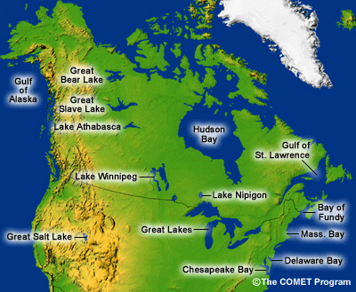
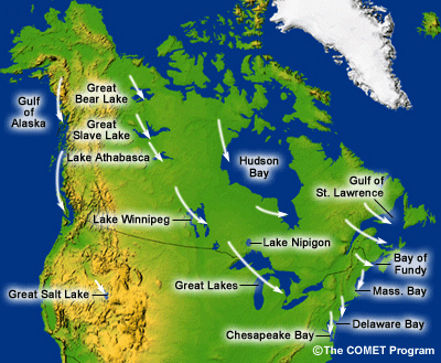
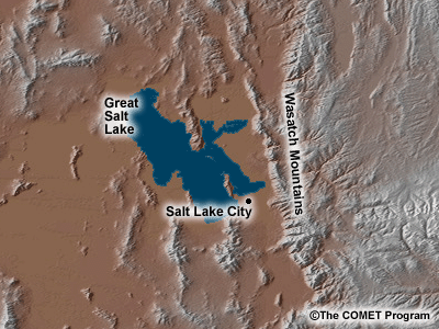
Only large bodies of water can generate instability of a scale sufficient to produce lake/ocean effect snow. In North America, lakes large enough to create lake effect include the five Great Lakes that border the U.S. and Canada, Great Bear Lake and Great Slave Lake in Canada’s Northwest Territories, Lake Winnipeg in Manitoba, Lake Nipigon in Ontario, Lake Athabasca in Saskatchewan, and the Great Salt Lake in Utah. Bay effect snow can occur in several areas including Chesapeake Bay, Delaware Bay, Hudson Bay, the Gulf of St. Lawrence, and the Bay of Fundy.

In general, smaller bodies of water do not create instability of sufficient scale to generate lake/ocean effect, but in a few locations such as in the Finger Lakes of upstate New York, localized lake effect snowfalls can occasionally occur.

Sources of Warm-Water Surface Temperatures and Moisture (cont.)

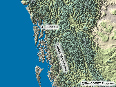
All of these warm water sources for lake/ocean effect snow also share the characteristic that they are situated in areas over which cold polar or arctic air masses frequently migrate in the cool season, which makes them climatologically favorable for the occurrence of lake/ocean effect snow. Ocean/land interfaces are also potential locations for events similar to lake effect snow. In some cases, such as near Juneau, Alaska, over Vancouver Island, British Columbia, and along the northern New England coast, ocean effect snow can occur when cold continental polar air masses pass over limited portions of warm ocean water before once again reaching land.

Sources of Warm-Water Surface Temperatures and Moisture (cont.)

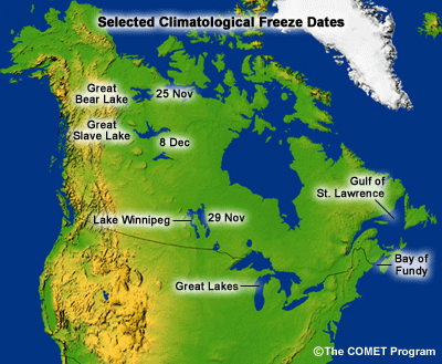
The lake/ocean effect process can occur any time that the overlying air mass is sufficiently colder than the water surface, but the occurrence of snow typically commences in November for the lower Great Lakes, and earlier at higher latitudes. As the cold season progresses, the water surface freezes on most northern lakes, and on some of the Great Lakes (e.g., Lake Erie and substantial portions of Lake Huron), cutting off the heat and moisture source and effectively ending the lake effect snow season. The higher the latitude and the smaller and shallower the body of water, the earlier this freezeover will occur. For many of the northernmost lakes, this keeps the lake effect season relatively short. For the Great Lakes, where freezeover dates are highly variable (if freezeover occurs), the NOAA Great Lakes Environmental Research Laboratory provides current water surface temperatures on their Website (http://www.glerl.noaa.gov/). In Atlantic Canada, the typical partial freeze-up of the Gulf of St. Lawrence will diminish the intensity of ocean effect snowfall by the mid-winter months. However, open leads can still produce local ocean effect. The Bay of Fundy remains ice free throughout the year.

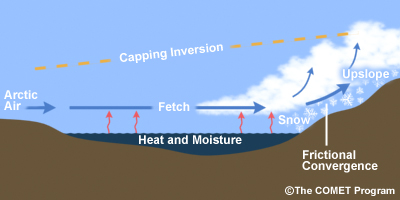
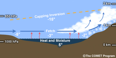
Characteristics of the Convective Boundary Layer

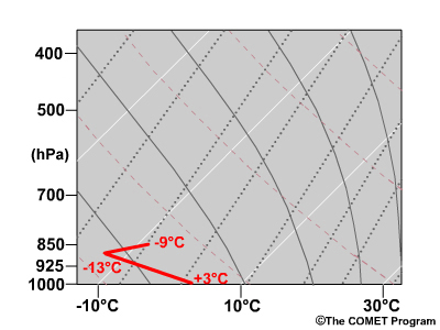
A defining characteristic of lake/ocean snow events is the generation of convection in the boundary layer. The formation of convective snow bands, with stronger vertical motions and enhanced precipitation production, results in limited areas of intense snowfall. An unstable lapse rate at low levels, brought about by heating and moistening by the water below, creates an environment favorable for convection. Typically, the temperature difference between the water surface and 850 hPa must be at least 13°C to support convective lake effect snowband formation in the Great Lakes. At higher elevations, such as the Great Salt Lake, a lake-to-700hPa layer is considered for determining the threshold temperature difference (16°C in this case). The threshold is basically determined by taking the dry adiabatic lapse rate from the lake surface to a particular reference level about 1.5 km above the lake. On some occasions, the capping inversion may occur below the reference level, but lake effect snow can occur provided the depth of the convective mixed layer exceeds 1 km. To assess instability thresholds, surface water temperatures are typically obtained from data buoys or satellite water temperature measurements. Particular care must be taken to obtain accurate values, since numerical model simulations have shown that small differences in surface water temperature can have large impacts on snow production, with temperature changes as small as 2°C resulting in 30-40 percent differences in total snowfall (Niziol, 2002).

• 13°C difference sfc-850hPa (Great Lakes example)
• 16°C difference 850-700hPa (Salt Lake example)
• 16°C difference with shallow inversion (Atlantic Ocean example)

Characteristics of the Convective Boundary Layer (cont.)

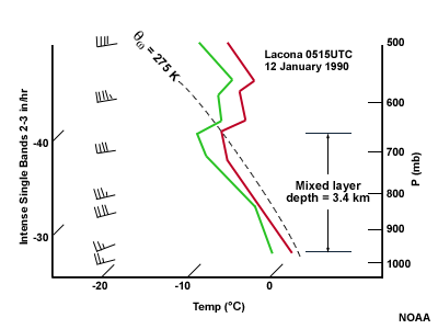
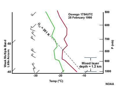
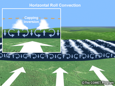
When assessing lake/ocean effect snow potential, the depth of the convective mixed layer must also be taken into consideration. In lake/ocean effect situations, a warmer air mass typically exists above the convective boundary layer. The resulting shallow cold layer and relatively low-level temperature inversion frequently limits the depth of the mixed layer, contributing to the formation of horizontal roll convection and multiple snow bands. However, mixed layers of less than 1 km are unlikely to generate convective processes sufficient to produce significant lake effect snow. By contrast, deep mixed layers (> 3 km) may help generate heavy snow in a single, more intense band dominated by more robust land breeze and frictional convergence processes, especially if the winds are oriented parallel to the long axis of an elliptically shaped water body (e.g., Lake Ontario).

• Single Band
• Multiple Band

Characteristics of the Convective Boundary Layer (cont.)

In addition to the unstable thermal lapse rate, low-level moisture from evaporation off the water surface further enhances the instability as the air moves across the lake, bay, or ocean. As the cool season progresses, the water surface may freeze, reducing or cutting off the heat and moisture source.

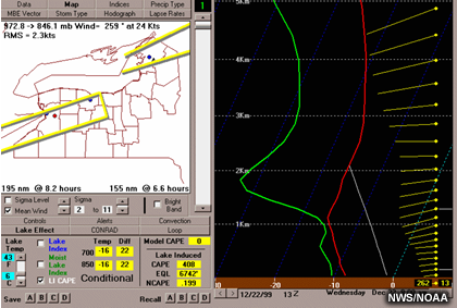
While rules of thumb regarding water surface and atmospheric temperature differences are useful, a more complete picture of the potential for lake/ocean effect snow is given with parameters such as “lake induced CAPE” and “lake induced equilibrium level” (LIEL). These can be calculated within a sounding tool, such as that contained within Bufkit (https://training.weather.gov/wdtd/tools/BUFKIT/index.php), that allows you to plug in a user-specified surface temperature and dewpoint, defined by taking into account the surface water temperature. (Note the calculated Lake Induced CAPE, EQL, and NCAPE in the bottom center of the Bufkit window.)

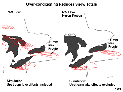
Upstream Conditioning

Additional boundary-layer heat and moisture can be supplied by upstream bodies of relatively warm water and by higher upstream relative humidity. The additional heat and moisture can condition the downstream air mass and may enhance precipitation production, as is shown by the increased model-simulated precipitation maximum southeast of Lake Ontario in Example 1. This is another reason, in addition to fetch distance over the downstream water body, that wind orientation can make a significant difference in the amount of snow produced. In some instances, however, model simulations show that upstream warm water sources may actually over-condition the air, relaxing the heat and moisture gradients between land and water areas, as shown by the reduced precipitation maximum to the east of Lake Ontario in Example 2. This acts to reduce the land breeze convergence that fuels snowband and subsequent snowfall production. This effect is maximized early in the lake/ocean effect season, when the surface water temperatures are still relatively high.

• Example 1
• Example 2

Lifting Mechanisms

Lifting Mechanisms in Lake/Ocean Effect Snow Events:

• Orographic lift
• Frictional convergence
• Thermal convergence

Once boundary-layer instability over the water has been enhanced by moistening and warming, several mesoscale mechanical lifting mechanisms may help to trigger and/or enhance the convective processes. These mechanisms include terrain or orographic lifting, frictional convergence, and thermal convergence. While such lifting mechanisms are not strictly required for the occurrence of lake/ocean effect events, they are observed in most instances. In addition, synoptic-scale lift ahead of a migrating mid-tropospheric shortwave trough may also add sufficient impetus for the convective process.

Orographic Lift

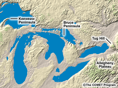
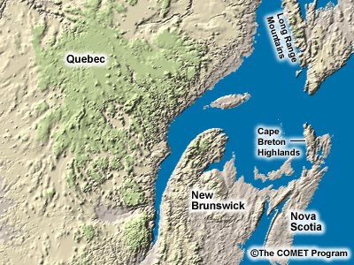
As the air travels from the water surface over land, some orographic lift is often involved. In some locations, however, terrain plays a major role lake/ocean effect snow production. For the Great Lakes this would include locations such as the Keewenaw Peninsula of Michigan, the Bruce Peninsula in southern Ontario, the Tug Hill and Allegheny Plateaus of upstate New York; for the Great Salt Lake, the Wasatch Range; for Atlantic Canada, the Long Range Mountains in Newfoundland and the Cape Breton Highlands in Nova Scotia; and for the Alaska panhandle, the Coast Mountains. It is estimated that annual snowfall increases by 65 cm per 100-meter elevation gain leeward of the Great Lakes.

• Great Lakes
• Canadian Maritimes
• Great Salt Lake
• Alaskan Panhandle

Frictional Convergence

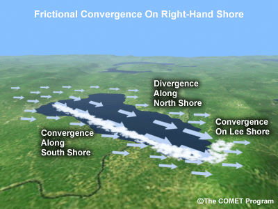
Surface winds moving over water experience very little frictional drag, so wind speeds are relatively higher than those over land surfaces where hills, vegetation, and even large buildings can reduce wind speed. As a result, fast-moving air over the water converges into slow-moving air over the land creating a zone of frictional convergence and lift near the leeward shore. The opposite effect occurs along the windward shore, resulting in surface frictional divergences and subsidence. In addition, the winds over land are slowed to a greater extent by friction resulting in a larger leftward deflection across isobars towards lower pressure than that occurring over the water. Therefore, relative to the prevailing low-level wind flow, frictional convergence is favored near the right-hand shoreline, and this can be the dominant factor in creating a single band of convection near the shore. Over time this band may propagate inland away from the original zone of convergence.

Thermal Convergence

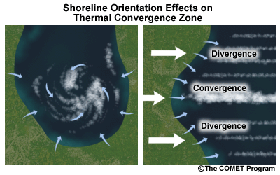
An additional source of convergence and lift is brought about by the land breeze generated by the thermal gradient between the lake and adjacent land areas. The relatively warm, moist environment over the water contributes to the formation of a “mesolow” that enhances the convergence of cooler land breezes over the water body. The cooler land breeze helps to lift the unstable air over the water, and this lifting can be particularly significant in cases where land breezes from opposite shores converge in the vicinity of the mesolow.

Thermal Convergence (cont.)

At times, the position of this band may be near the shoreline, similar to the location of the band created by frictional convergence when the larger-scale background flow forces the convergence zone closer to the leeward shore. This suggests that in certain instances multiple convergence mechanisms may be working in concert to enhance the lifting.

Thermal Convergence (cont.)

When the background flow is relatively light, the shape of the shoreline can influence the shape of the resulting convection. A land breeze over a deep bay or bowl-shaped portion of a lake can create a lake meso-vortex, while a shallower bay may act to simply focus the thermal convergence producing a dominant band in a multiple band scenario.

Fetch, Wind Speed, and Shear

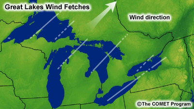
Fetch

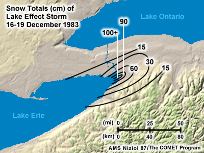
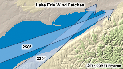
The distance that cold air travels over the relatively warm water, known as the fetch, is very important in the formation of lake/ocean effect snow bands. The minimum threshold for flurries appears to be about 80 km, but a minimum fetch of 160 km is generally needed to produce significant lake/ocean effect snowfall. In the Great Lakes region, the fetch is usually determined operationally by the 850hPa wind direction, except in cases where the capping inversion falls below that level, when the 925hPa wind direction might be more appropriate. In higher elevations, such as the Great Salt Lake, the 700hPa wind direction is a much better indicator for the fetch. Note that small variations in wind direction can result in significant changes in fetch. On Lake Erie for instance, a 230 degree wind has a 130-km fetch, while a 250 degree wind results in a 360-km fetch!

• Lake Erie Fetches
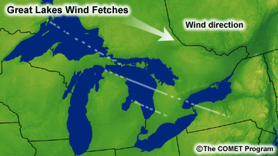
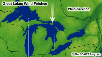
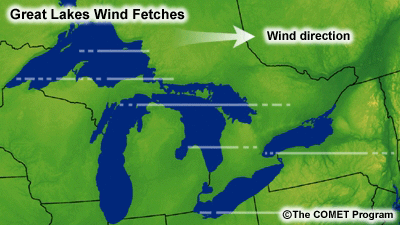
• Great Lakes Fetches

Lake Erie Fetches

Great Lakes Fetches

• Northwesterly Winds
• Northerly Winds
• Westerly Winds
• Southwesterly Winds

Wind Speed and Wind Shear

Wind speed is also important in the lake/ocean effect process. If wind speed is too strong, > 25 knots in the surface-to-850hPa layer (this layer will be different with elevated terrain), parcel residence time is limited, and the efficiency and organization of horizontal rolls may be disrupted. Stronger winds also distribute the snowfall to locations farther inland from the water body. When the wind speed is light, < 10 knots sfc-to-850hPa, land breeze circulations tend to dominate, often preventing the most intense lake/ocean effect snow bands from forming. The optimal surface-to-850hPa wind speed is about 15 to 20 knots, as this tends to maximize the parcel residence time, as well as the sensible (heat) and latent (moisture) flux from the warm water surface.

For optimal production of linear, lake effect snow bands and horizontal convective rolls, the winds in the mixed layer must be well aligned. Generally, the low-level wind direction should vary less than 30 degrees within the mixed layer for the formation and maintenance of intense snow bands. If the directional shear is greater than 60 degrees, lake/ocean effect snowband formation usually will not occur.

Wind Speeds
(kts)	Description
10	land breeze circulations dominate
15-20	optimal for lake/ocean effect snow bands
25	snow bands unlikely to organize

Wind Shears
° of Directional Shear	Description
0-30	optimal for more intense bands
30-60	weaker, less organized bands
> 60	band formation disrupted

Cloud and Precipitation Microphysics

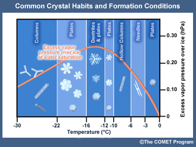
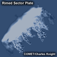
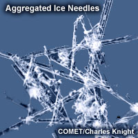
Ice Crystal Formation and Growth by Deposition, Accretion, Riming, and Aggregation

Temperatures within the cloud layer can play an important role in enhancing the precipitation production process and determining ice crystal structure in lake effect snow events. In a cloud environment supersaturated with respect to ice, water vapor deposition on ice nuclei will occur, and its rate is maximized at temperatures near -15°C. Once the ice crystals fall to lower portions of the cloud, they may contact supercooled water droplets which, in turn, freeze on the crystals by the process of accretion.

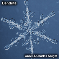
Growth of dendrites is maximized in supersaturated environments at temperatures between -13 and -16°C, especially in an area of enhanced upward motion. Riming typically occurs on crystals at warmer temperatures, generally greater than -10°C. Graupel is formed by extensive riming on crystals in supersaturated environments in this temperature zone. Larger snowflakes can form when ice crystals collide and stick together via the process of aggregation, also favored at temperatures > -10°C. The heaviest snowfall tends to occur in environments favorable for riming, dendrites, and graupel production.

Seeder-Feeder Process

Middle- and high-level clouds that produce ice crystals can serve to “seed” the lower lake/ocean effect clouds below. In this process, ice crystals generated in the higher clouds fall into the lower clouds allowing further snowflake growth by aggregation. This can enhance the precipitation production and lake/ocean effect snowfall.

Synoptic Setting

Overview

An analysis of the synoptic setting is critically important because current operational NWP models cannot fully resolve lake/ocean effect snow bands, especially in the medium time range (2-4 days) and beyond. On the other hand, the synoptic picture is generally well-depicted by these models. In order to better anticipate these events, the forecaster needs to have a good understanding of what synoptic patterns are conducive to lake/ocean effect precipitation scenarios.

The synoptic scenario described on the following page, i.e., cold, post-frontal surface winds, leads to the highest snowfall rates induced by lakes/oceans. Normally, the very highest total snowfalls occur when favorable synoptic thermal and pressure patterns (those that initiate the lake/ocean effect snowfall) persist for many hours. In especially intense episodes, these synoptic patterns may remain in place for 2-3 days!

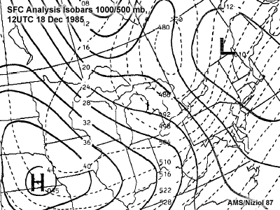
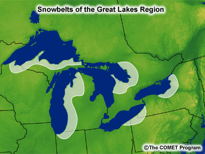
Favorable Synoptic Setting: Great Lakes

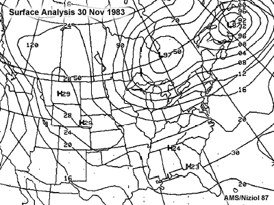
The post-frontal area behind (or generally west of, in the northern hemisphere) an exiting synoptic-scale trough or storm system is the most common synoptic region susceptible to the lake/ocean effect scenario.

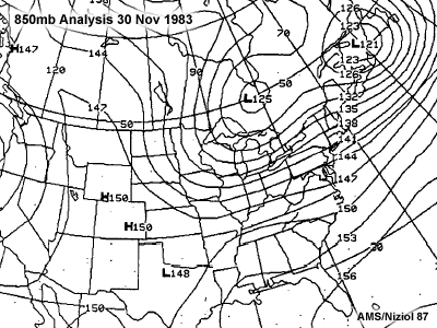
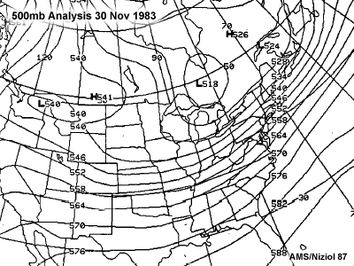
In the accompanying 500hPa analysis, favorable lake effect conditions are present over western New York State. Note the NNW/SSE-oriented gradient flow present in this region and the low pressure trough off to the east. Also, extremely cold thickness values are present over and upstream of the eastern Great Lakes region.

The reason that this area is favorable for lake effect snowfall is that low-level cold advection usually sets in behind a storm system. Cold advection can create a situation where cold continental air is flowing over a warm body of water. Over the northern hemisphere, this is most common in a northwesterly synoptic wind situation at the surface (and MSLP isobars aligned in the NW-SE direction, as in the New York State lake effect case mentioned above), but the scenario can occur under varying directions from southwesterly through northerly and even easterly (see Great Lakes Snowbelts figure). Low-level cold advection also is conducive to the formation of a synoptic-scale inversion at the top of the cold air mass. The snowbelts depicted in the accompanying figure are in locations corresponding to downstream locations during post-frontal conditions. (“Downstream” can refer to areas northeast, east, or southeast of the Lakes.)

• Favorable Synoptic Setting
• Great Lakes Snowbelts

Another Great Lakes Example

This is another example of a favorable lake effect situation to the east of Lake Erie and Lake Ontario. In this case, persistent post-frontal westerly flow produced a very heavy lake effect event. In this case, there was very little directional shear from the surface up to 500 hPa, and the westerly flow produced long fetches over both lakes, resulting in the formation of intense, single snow bands.

• Surface Analysis
• 850hPa Analysis
• 500hPa Analysis

Aggregate Effect of the Great Lakes

The Great Lakes are large bodies of warm water that feed back onto synoptic-scale processes. This is often manifested in an alteration of the MSLP field in which cyclonic curvature persists after the northerly flow behind a storm system is set up. The persistence is noted both at the surface and middle levels of the atmosphere. This feedback contributes positively to the rate and persistence of Great Lake effect snowfall.

This effect also results in the formation of additional low pressure zones downstream of the water bodies. In addition, the aggregate effect may alter synoptically-induced precipitation distributions by enhancing synoptic uplift in preferred regions. In other words, the regional flow characteristics are altered enough by the water bodies to have direct effects on the synoptic details. In synoptic climatologies, the aggregate effect manifests itself as increased frequency of mid-tropospheric cyclonic flow.

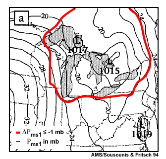
Thin lines are MM4-predicted MSLP contours at 48 hrs., and thick lines are differences in MSLP between simulations with and without the Great Lakes. Note the presence of a synoptic-scale pressure anomaly exceeding 1 hPa over and northeast of the Great Lakes.

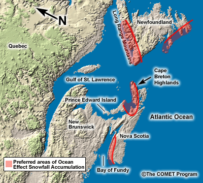
Favorable Synoptic Setting: Atlantic Canada

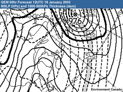
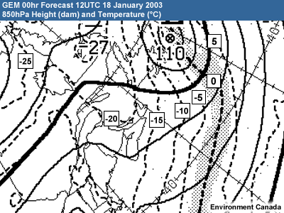
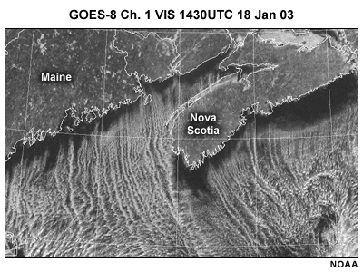
The post-cold-frontal scenario is the most common synoptic pattern for ocean effect snowfall over Atlantic Canada. Extratropical low pressure systems heading eastward to the Atlantic Ocean sweep cold polar or arctic continental air across the region in their wake. The accompanying surface and 850hPa charts illustrate a typical example. The cold front associated with the 976hPa low just east of Newfoundland has moved well to the south of the Nova Scotia coast ushering in a cold north-to-northwesterly airstream across the still mostly ice-free Gulf of St. Lawrence, the Bay of Fundy, and the Atlantic. From the accompanying 850hPa height-temperature chart it can be seen that the temperatures at 850hPa range from –15°C just off the Nova Scotia coast to below –20°C over the Gulf of St. Lawrence. The ocean temperatures range from close to freezing over the Gulf of St. Lawrence waters to the high single digits over the Atlantic to the south of Nova Scotia (near the northern boundary of the Gulf Stream). Hence the temperature difference threshold of 13°C is exceeded over all three water bodies. The resulting ocean effect snow bands are well-depicted in the available visible satellite image for 1430UTC.

• Surface Chart
• 850hPa Chart
• Satellite Image

Common Ocean Effect Locations in Atlantic Canada

Although northwest is the most common wind direction for ocean effect snow, wind directions from WSW through NNE can accompany cold polar outbreaks across the region. On more rare occasions, when an artic outbreak has swept sub-zero air well to the south of Nova Scotia and Newfoundland, a period of ocean effect snow can be generated by winds with a southerly component ahead of an approaching warm front. This can bring unexpected ocean effect snow to the relatively heavily populated areas along the Atlantic coast of Nova Scotia and the southeast coast of Newfoundland. The most common areas for ocean effect snow accumulation in Atlantic Canada are illustrated in the accompanying figure.

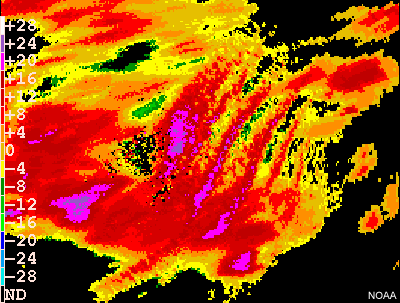
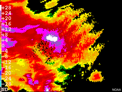
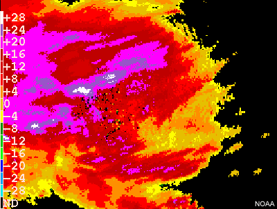
Role of Weak Synoptic-Scale Upward Motion

A background presence of upward motion due to synoptic-scale processes, such as warm advection aloft or differential vorticity advection aloft, can enhance the lake/ocean effect snowfall. In this situation, a combination of lake/ocean effect and synoptic-scale processes contribute to precipitation development. The most prevalent example of superposition of synoptic-scale uplift is in persistent mid-level cyclonic flow on the backside of a slowly-moving (or stationary) trough or cutoff low. The commonly used delta-T threshold of 13°C (sfc-850hPa reference) for significant lake effect may not apply during this situation, in which significant lake/ocean effect snowfall can occur with the temperature differences as small as 10°C. The available radar images depict an event in which synoptic-scale uplift is superimposed on existing ocean effect snow bands to enhance and broaden snowfall for a brief period of time.

The moisture content of the incoming low-level air, which can be enhanced in conditions of weak, large-scale uplift, is important to the nature and extent of the subsequent lake/ocean-induced precipitation development. Moist incoming winds generally lead to more widespread cloud and precipitation coverage downstream of the water bodies. Moisture content aloft is also important to the potential for seeder-feeder precipitation enhancement.

Also, studies have shown that cyclonic vorticity advection above the capping inversion can raise the inversion level over the boundary layer and subsequently enhance the lake/ocean effect snowfall by allowing deeper convection.

• 13UTC Radar
• 17UTC Radar
• 18UTC Radar

Lake/Ocean Enhancement: When Synoptic Forcing is Dominant

A favorable fetch of the low-level wind, produced by a synoptic-scale storm system and in the precipitation-producing portion of the storm, can enhance snow production when it happens to be over a warm body of water, even when lake/ocean effect convective processes do not occur. In this case, additional destabilization occurs as heat and moisture are transported upward into the low-level air in the same way that pure, direct lake/ocean effect processes begin. In such lake/ocean-enhanced snow situations, however, the synoptic uplift is dominant, and the contribution of the lake or ocean is simply to add to the resulting snow amounts.

Snow Banding Processes

Types of Lake/Ocean Effect Snow Bands

Lake/Ocean effect snow bands tend to develop parallel to the prevailing wind flow in the lower tropospheric mixed layer, and typically occur as either a prominent single band or an area of smaller, multiple bands. Single bands tend to exhibit greater intensity and heavier snowfall over a narrow area, while multiple bands tend to be associated with lighter snowfall over a larger area. There are also less frequent occurrences of snow bands exhibiting characteristics similar to both single and multiple bands, and in rare cases a mesoscale vortex may develop near one end of an elongated body of water. Slight differences in the wind direction, and therefore the synoptic setup, can change the snow band location and behavior dramatically.

This animation of GOES visible imagery shows a particularly active lake effect snow event in progress involving all of the Great Lakes. Multiple bands appear evident over most of the lakes with the exception of single snow bands, oriented northwest-to-southeast over northern Lake Huron, and oriented west-to-east over Lake Ontario.

Single Snow Bands

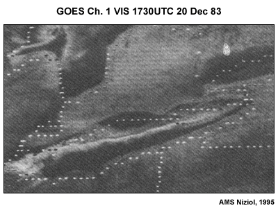
Single, wind-parallel snow bands generally develop when the prevailing low-level flow is more nearly parallel to the long axis of an elliptically-shaped lake or bay (see Conceptual Model). For example, single band development is preferred with west winds over Lake Ontario, north winds over Lake Michigan, north-northwest flow over Lake Winnipeg, and so on. These bands typically develop over the center of the warm water body, fueled by organized low-level land breeze convergence from both shores. The resulting single snow band is typically 20-50 km wide and 50-200 km in length and can produce snowfall rates exceeding 10 cm/hr.

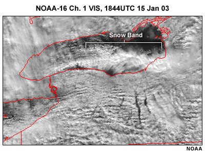
The GOES visible imagery example here focuses on the large single snow band that formed over Lake Ontario during the morning hours of 15 January 2003 and persisted for nearly 12 hours. During the height of the event, snowfall rates within the snow band were as heavy as 7-15 cm/hr (3-6 in/hr). Storm totals for the event in portions of Oswego county east of Lake Ontario approached 1 m (3 ft).

Single bands may migrate to one shore if the prevailing winds are at a slight angle to the major axis of the water body. In the conceptual example over Lake Ontario, west-southwest winds may result in a snow band along or near the north shore, west winds favor a snow band over the center of the lake, while west-northwest flow results in a snow band near the south shore.

• Example
• Conceptual Model

Special Single-Band Case With Light Winds

Occasionally, a single shore-parallel band may set up under quiescent conditions associated with a very cold, arctic high pressure system. With very light winds due to the relatively weak low-level pressure gradient, thermal convergence dominates, and a mesocale land breeze may set up a convective snow band under the dome of the arctic high. In these situations, synoptic-scale subsidence usually limits the convection, and the snow band my penetrate only a short distance inland due to the light prevailing wind flow. However, these snow bands generally have high snow-to-liquid ratios and may therefore produce significant snow accumulations (15 cm or more), especially if the synoptic conditions persist and the band remains over one location for several hours. These bands are often difficult to forecast, given that they typically occur under conditions of synoptic-scale subsidence and depend on the shoreline configuration and development of a land breeze circulation.

• Conceptual Model
• Example

Multiple Snow Bands

When the prevailing wind flow is across a shorter fetch of water or more nearly normal to the major axis of an elliptically-shaped water body (e.g., northwesterly flow across Lakes Superior and Huron, west-northwestly flow across Lake Winnipeg), multiple wind-parallel bands may form. Since the shorter fetch limits the heat and moisture fluxes, these multiple bands generally occur with relatively shallow (< 1.5 km) convective mixed layers and are driven by horizontal roll convective circulations. As a result, despite the fact that they affect a much larger area than single bands, the convection is weaker, and the resulting snowfall rate at any point is considerably less. The multiple bands are typically a few km to 20 km wide and 20-50 km long.

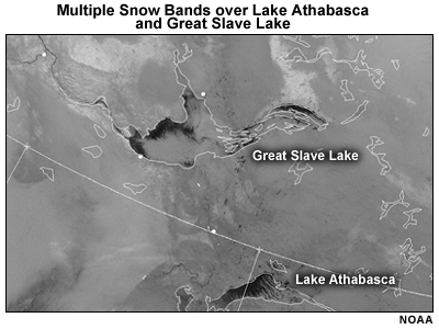
In Example 1, the GOES visible satellite image shows north-northwest to south-southeast oriented multiple bands resulting from horizontal roll convection south of Quebec and Nova Scotia. Example 2 shows northwest-to-southeast oriented snow bands over Great Slave Lake in northwest Saskatchewan and Lake Athabasca in the Northwest Territories.

• Conceptual Model
• Example 1
• Example 2

Hybrid Snow Bands

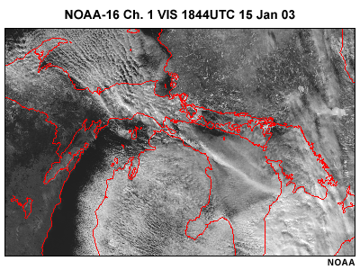
Snow bands generated by an upwind body of water may re-intensify over a downwind water body and can consist of single or multiple bands. For example, bands may develop over Lake Superior, move across Michigan, and then re-intensify over Lake Huron and bring significant snowfall to southwestern Ontario. Once these bands move inland from the upwind body of water, they may appear to dissipate, but their low level moisture channel and convergence remains intact, enabling them to re-intensify over the downwind water body. Because these snow bands often exhibit little spatial or temporal persistence and affect areas far removed from their source regions, they pose a particularly difficult forecast challenge.

This visible image taken by the NOAA-16 polar-orbiting satellite shows multiple snow band activity as it moves southeast of Lake Superior and then reorganizes into a single band over Lake Huron. Amazingly, this single snow band persisted across the length of Lake Huron, depositing snow as it made landfall near Southampton in southwestern Ontario.

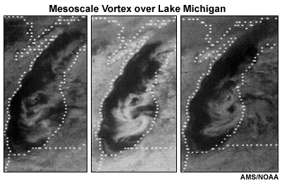
Mesoscale Vortex

On rare occasions with an arctic high, light winds, and strong subsidence above the convective mixed layer, a mesoscale vortex may form. The mesoscale vortex will usually have spiral bands extending out from its center, as shown by the visible satellite image

Mesoscale vortices usually form near the end of elliptically-shaped lakes where the coastline has a “bowl-shaped” orientation. Thermal (land-breeze) convergence develops as a result of the bowl-shaped orientation and generates a vortex cloud band structure. Despite their somewhat ominous appearance, mesoscale vortices typically produce only small amounts of snow, and are most frequently observed over Lakes Superior, Huron, and Michigan.

• Conceptual Model
• Example 1

Satellite Imagery for Detection

Challenge of Detection

Since intense lake/ocean effect snow bands can have widths as small as a few kilometers and are inherently low-topped convection, they are often difficult to detect. Even in populated areas with good radar coverage and a high density of surface observations, the snow bands may fall between surface observation sites, and even the lowest-level radar scans may overshoot the precipitation at ranges beyond 100 km. In higher-latitude regions with no radar coverage and sparse surface observations, detection is even more problematic.

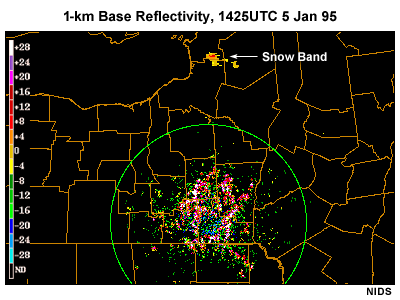
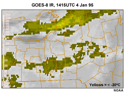
The two figures shown here compare radar and satellite observations of a large single snow band over Lake Ontario during a heavy lake effect snow case on 4 January 1995. The reflectivity scan taken at 0.5 degrees elevation is shown for the Binghamton, New York radar at nearly the same the time as the GOES-8 infrared image. Reflectivity values observed with the snow band are more than 150 kilometers from the radar site, which means that the radar beam is observing reflectivity values at more than 1.4 kilometers above ground level, well above the maximum reflectivity values associated with this event (600-800 meters). As a result, the snowband is poorly depicted by radar, despite being easily identified in the GOES-8 infrared image.

While an integrated approach to detection using a variety of platforms (surface data, radar, satellite, etc.) is optimal, GOES and POES satellite imagery will often be the primary means for detecting the bands, especially in the far northern locations.

• Radar
• Satellite

Satellite Channel Selection for Lake Effect Detection

Water vapor imagery is useful to infer large-scale flow patterns and track upper-level short waves that may enhance lake/ocean effect snow bands. This water vapor animation shows a mid- and upper-level short wave as it moves rapidly across the Great Lakes region during a lake effect snow event. The short wave is embedded within strong northwesterly flow as it rotates into the base of a deep, large-scale wintertime trough. Snow band activity is benefiting from both the enhanced upward lift present along the leading edge of the short wave and a further destabilization of the environment resulting from upper-level cold air advection accompanying the short wave.

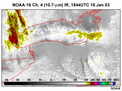
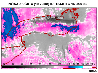
Visible imagery can readily depict snowband locations during the daytime, and the 10.7-µm infrared imagery can depict regions of cold, cloud top temperatures to infer convective band intensity. A water body appearing relatively bright on visible imagery is usually indicative of an ice surface, indicating little or no potential for lake/ocean effect snow bands. The NOAA-16 visible and 10.7-µm IR imagery available here illustrate how conventional infrared imagery, when properly enhanced, is able to isolate the deeper convective elements within a single snow band. Notice how cloud tops are progressively colder in the downwind direction of this Lake Ontario snow band, indicative of heavier snowfall rates at the surface.

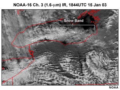
A shortwave infrared channel capability available with the current NOAA-AVHRR, Terra and Aqua-MODIS polar-orbiting imagers improves detection of lake effect snow bands over land in the presence of snow-covered ground and when animations are unavailable. The NOAA-16 visible and 1.6-µm shortwave IR imagery available here illustrate how easily snow band activity can be distinguished from snow covered ground along the shores of Lake Ontario and eastern Lake Erie. Similar shortwave imaging channels will come on line with the next generation POES (NPOESS and METOP) and GOES (GOES-R) satellites.

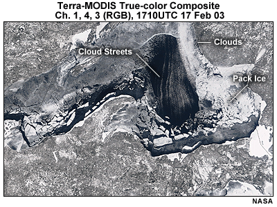
A water body appearing relatively bright on visible imagery is usually indicative of an ice surface, indicating little or no potential for lake/ocean effect snow bands. Standard visible imagery still offers one of the best approaches to determining the extent of ice cover over known lakes. Three visible channels of the MODIS imager (onboard the Terra satellite) have been combined into this 500-meter resolution true-color composite image. The available image shows extensive pack ice, which formed over Lake Superior following a two-week period with average temperatures below -20°C. Notice that an area of cloud streets has formed over a portion of eastern Lake Superior that remains open. When low clouds move over snow and ice surfaces and contrast is lost in the visible, analysis of shortwave imagery greatly enhances the detection of low cloud features.

• Water Vapor
• MODIS True-color Composite
• Visible/10.7-micrometer
• Visible/1.6-micrometer

Water Vapor

MODIS True-color Composite

Visible/10.7-micrometer

Visible/1.6-micrometer

Satellite Imagery for Microphysical Information

Satellite imagery can also be used to infer microphysical properties within lake/ocean effect cloud bands. Infrared cloud top temperatures below -15°C imply efficient precipitation production and a greater likelihood for intense lake/ocean effect precipitation. The available 10.7-µm image uses a special enhancement table to highlight cloud-top temperatures between -15 and -30°C (pink). The rate of crystal growth typically reaches a maximum at temperatures around -15°C. Cloud tops colder than -30°C are shown in blue. Near the eastern shores of Lake Ontario, cloud tops transition from pink to blue indicating the presence of deeper convection and the likelihood of greater snowfall rates.

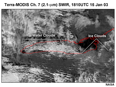
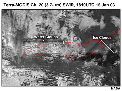
Imagery from the shortwave infrared channels on GOES and POES satellites allows one to infer liquid water and ice content in clouds. In the available shortwave infrared example, the 2.1-µm channel (nearly identical to the 1.6-µm channel and also used for cloud discrimination) highlights cloud top hydrometeors associated with a large Lake Ontario snowband as relatively bright. Surrounding water and land surfaces appear poorly reflective and relatively dark. The grayer appearance of cloud tops within the band closer to land hints at the presence of ice. For a more definitive answer to the liquid vs. ice cloud top question, we can fade to the 3.7-µm image. The daytime 3.7-µm shortwave infrared channel continues to show liquid water clouds as bright reflectors, but glaciated ice crystal clouds are now shown as poor (dark) reflectors. The locations where cloud tops transition from liquid to ice (transition from light to dark near the lee shorelines of Lakes Huron, Erie, and Ontario) are areas where efficient precipitation production and heavy snowfall may be occurring.

• 10.7-micrometer
• Shortwave Infrared

10.7-micrometer

Shortwave Infrared

Winter Precipitation Processes

Ice Crystal Growth

Three Ice Crystal Growth Processes

Once an ice crystal has formed, it can grow through several processes:

• diffusion deposition
• accretion
• aggregation

Depending on the temperatures and saturation levels in the cloud, the ice crystal can grow in various forms, or crystal habits. Of course, if the ice crystal travels to areas warmer than 0°C, it can also melt.

Ice Crystal Growth by Diffusion Deposition

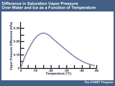
Diffusion deposition occurs due to differences in the saturation vapor pressure between ice and liquid water. At a given temperature, the vapor pressure over a water surface is greater than that over an ice surface. If water droplets and ice crystals exist in the same environment (called mixed phase conditions), a vapor pressure gradient develops between the droplets and crystals. Due to this gradient, water vapor moves from the higher pressure surrounding the droplets to the lower pressure surrounding the crystals. Thus, the ice crystals grow at the droplets' expense. This process creates sub-saturation with respect to water, and the droplets evaporate to maintain water saturation, making additional water vapor available for ice crystal growth. Eventually the pool of liquid water diminishes and the cloud becomes glaciated.

The process of growth by deposition can also take place in a setting that is supersaturated with respect to ice as the ice crystals continue to grow through deposition of the free water vapor surrounding the ice crystals.

Ice Crystal Growth by Diffusion Deposition (cont.)

The rate of growth of ice crystals is most directly influenced by temperature and humidity. Lowering the temperature of a cloud causes conversion to ice and existing ice growth to speed up at the expense of any available liquid water.

The rate of diffusion is highest where the difference between the saturation vapor pressure between ice and supercooled liquid water is greatest. Optimal growth rates occur near -15°C.

Ice Crystal Growth by Accretion (Riming)

In a process called accretion, ice crystals can grow via collision with supercooled droplets. The supercooled droplet freezes on contact and sticks to the original ice crystal to form rime ice. This process is optimal in saturated layers with temperatures of 0 to -10°C (Staudenmaier, 1999). Excessive riming eventually results in the formation of graupel or snow pellets.

Ice Crystal Growth by Accretion (Riming) (cont.)

As ice crystals grow by accretion, rapid freezing of droplets can result in shattering to form multiple tiny ice particles. This process is called splintering and is a secondary source of ice-forming nuclei (IN). This can then speed up the accretion process and glaciation of the cloud.

In summer convective storms, hail is formed as heavily-rimed ice crystals are continuously swept up into regions of supercooled drops in the convective cloud, growing in the cycling process until their weight overcomes the updrafts.

Ice Crystal Growth by Aggregation

As ice crystals grow and collide, they can stick to each other in a process called aggregation. Liquid molecules on the outer surface of the crystals serve to increase bonding between two colliding crystals. As the crystal moves through warmer regions in the cloud, there will be more liquid molecules on the outside of the crystal, and larger aggregations can build to form large snowflakes. Stickiness is maximized at or near 0°C.

Crystals with dendritic characteristics can also mechanically interlock to form larger aggregates (Pruppacher and Klett, 1979).

The Ice-Crystal Process: Operational Significance

Operationally, knowledge of the ice crystal process can help in forecasting precipitation type and amount and is essential in making aviation icing forecasts. The following topics summarize the operational implications of the ice crystal process.

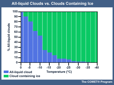
Ratio of Supercooled Cloud to Mixed Phase

Within clouds, at temperatures warmer than -10°C, supercooled liquid can be expected most often. Generally, with decreasing temperature, the likelihood of the cloud containing ice increases. At -20°C, fewer than 10% of the sampled clouds consisted entirely of supercooled liquid.

Optimal Temperatures and Conditions for Ice Crystal Initiation and Growth

Observation and laboratory experiments indicate that the optimal conditions for ice crystal initiation and growth are in cloud layers that are saturated with respect to liquid water, and thus supersaturated with respect to ice, with temperatures in the -10 to -18°C range.

Potential Presence of Ice Crystal Initiation

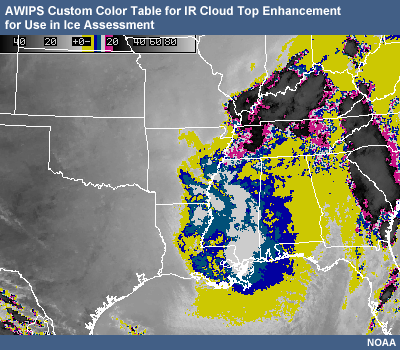
AWIPS can be used to highlight the liquid-to-ice temperature range in cloud tops. Based on cloud-top temperature, and the color regimes in the table below, the presence of ice in cloud tops can be determined through the use of IR.

Potential presence of ice crystal initiation in clouds based on temperature
Temp. (°C)	Potential Presence of Ice Initiation
0	no initiation
-4	no initiation
-10	60% chance
-12	70% chance
-15	90% chance
-20	100% chance

• Color Table Information
• Sample AWIPS IR Image

Color Table Information

Enhancement Color	Temperature Deg (°C)	Ice or Liquid	Optimal AWIPS color choices (RGB values)
Yellow	0 to -8	Liquid	255  255   0
Blue	-8 to -10	Likely Liquid	0     0     200
Light Blue	-10 to -12	60% Chance Ice is there	0   100   150
White	-12 to -15	70% Chance Ice is there	255  255  255
Pink	-15 to -20	90% Chance Ice is there	250  0 160 (-15°C) interpolated to 250  80  170 (-20°C)
Black to White	-20 or less	ICE is there!	0  0  0 (-20°C) interpolated to 255  255  255 (coldest temp)

Sample AWIPS IR Image

.

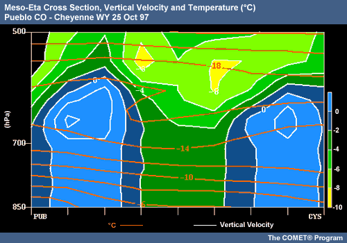
Dendrite Zones and Heavy Snowfall

Regions of the atmosphere where upward vertical motion coincides with temperatures favorable for dendritic growth (-12 to -16°C with high RH values) are strongly correlated wtih heavy snowfall. Crystal growth rates and aggregation are maximized in dendrtic zones. Upward vertical motion in regions of high RH replenishes the supply of supercooled liquid water droplets and thus enables rapid dendrite growth to continue.

This cross section from Pueblo, Colorado to Cheyenne, Wyoming on 25 October 1997 shows an example of this effect. Heavy snows were observed in the Denver area, the central region of this cross section. Relative humidity throughout this region was > 90% at the time. Note the location of high vertical velocity both within and above the -12 to -16°C layers. In the layers above, where vertical velocity is highest and temperatures are lower (-17 to -20°C), smaller crystals would be forming and falling through the dendritic zone below, rapidly growing through aggregation and developing into larger dendrites.

Aviation Icing Threat

The presence of cloud layers composed of supercooled liquid poses a potential icing threat to aircraft passing through those layers. Cloud layers consisting of ice particles pose no icing threat.

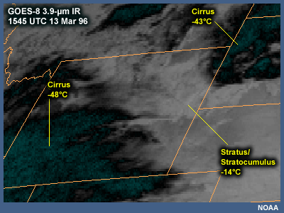
Use of GOES 3.9 to Determine Cloud Phase

Clouds consisting of ice particles can be distinguished from clouds consisting of supercooled water droplets through examination of the GOES 3.9-µm infrared imagery. At this wavelength, reflectance by water droplets is much greater than the reflectance from ice particles. Therefore, lower clouds (stratus or stratocumulus) containing water droplets appear white, while the higher clouds (cirrus) containing ice particles appear dark. This is opposite from the normal appearance of high and low clouds on a channel-4 IR image. In this image, lower-level water droplet clouds are evident over northeast Wyoming, while higher-level ice crystal clouds are evident over southwest Wyoming, northern Colorado, and South Dakota.

It is important to note that upper-level ice clouds can obscure lower-level supercooled liquid clouds in satellite images.

Characteristics of Natural Cloud Seeding

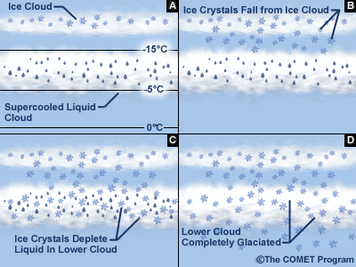
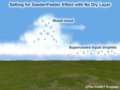
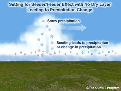
Natural Cloud Seeding: The Seeder/Feeder Effect

Natural cloud seeding, also known as the seeder/feeder effect, is a common occurrence in many cold weather settings. Ice phase clouds may induce ice crystal formation, and subsequent precipitation, in supercooled clouds below them. This can happen when ice crystals in the upper cloud fall into the lower cloud providing ice-forming nuclei (IN). If conditions are right, the seeding of ice crystals from above can enhance the precipitation process. In cold-weather conditions, this effect can significantly increase snowfall amounts.

If cold clouds containing ice crystals overlay a lower deck consisting of supercooled liquid, the lower deck can be depleted of liquid in as little as 20 minutes. This was observed in a case study in northeastern Colorado (Politovich & Bernstein, 1996), where liquid was quickly depleted in a low-level cloud by riming of ice crystals falling into it from aloft.

Common Settings for Seeder/Feeder Effect

Natural cloud seeding occurs quite frequently in certain settings:

• Middle- or upper-level clouds precipitate ice crystals to lower-level supercooled liquid clouds
• In orographic settings, enhanced bands of precipitation may form below mountain wave induced clouds if lower-level clouds are present
• In lake effect conditions, precipitation from lower-level lake-effect bands may be enhanced by overriding mid- or upper-level clouds
• Decoupled low-level upslope clouds may be seeded by mid-level precipitating (possibly convective) clouds

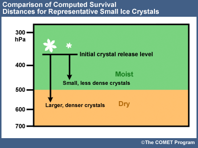
Distance Limit Between Feeder and Seeder

The limit to the seeder/feeder mechanism seems to be about 1500 m (5000 ft) (Hall and Pruppacher, 1976). That is to say, that the seeder (ice) cloud must be not more than about 1500 m above the supercooled liquid cloud (feeder).

The figure shows a few important features of ice crystals falling through and below the cloud:

• The authors state: "...ice crystals falling from cirrus clouds can survive fall distances of up to 2 km (about 6500 feet) when the relative humidity is below 70% in a typical midlatitude atmosphere.
• The larger the crystal, the longer it will survive—especially in a subsaturated environment.
• Crystals can fall over 2 km in near-saturated conditions, but after reaching RH < 70% in this study, the crystals rapidly disappear within about 1 km, taking at most 20 minutes to do so.
• Smaller crystals actually evaporated within a more saturated environment in the above scenario.

At distances greater than about 1500 m between two cloud layers, ice falling from the seeder will tend to evaporate/sublime before reaching the feeder cloud.

Distances between the layers can be tough to assess in real time away from sounding times and locations. Operational forecasters may want to use 3.9-µm IR channel 2 GOES imagery during daytime and the GOES Fog/Stratus at nighttime to assess water versus ice cloud tops.

WSR-88D VWP profile is useful in assessing the distance between cloud layers. On the VWP, wind barbs should be evident in both the seeder and feeder layers with the dry layer between them showing no barbs. This gap is measurable.

Seeder/Feeder With No Gap Between Layers

An analogy to the classic seeder/feeder situation occurs when the gap or dry layer between the clouds does not exist, but the lower cloud layer is decoupled from the deeper cloud layer.

In this situation, crystals falling from the deeper (possibly convective) cloud seed the lower cloud, which may be composed of water droplets. The lower cloud is relatively stationary, while the upper cloud is moving towards the east (Example 1).

In some situations, when the deeper cloud is moving, this effect leads to a precipitation changeover or enhanced snow production under the deeper cloud (Example 2).

Operationally, this means that a forecast of freezing rain or drizzle can run into problems when snowfall occurs due to an unforeseen seeder/feeder process. Check the satellite imagery to help this diagnosis and try to address it in the nowcast. Remember, GARP gives cloud-top temperatures by placing the cursor at a given location on 10.7-µm IR imagery.

• Example 1
• Example 2

Satellite Imagery for the Detection of Natural Cloud Seeding in Winter

AWIPS Satellite Color Enhancement Curve to Assist Ice Assessment

AWIPS and other satellite display systems can be used to highlight temperature ranges in cloud tops. Based on cloud top temperature, and using a color enhancement such as the one in the table below, the potential presence of ice in cloud tops can be determined through the use of 10.7-µm IR imagery. The presence of liquid at cloud top generally indicates that the entire cloud is predominantly liquid. This is particularly helpful for analyzing freezing drizzle environments with low stratus, which may have areas of more vertical development.

• IR Cloud Tops
• Table

IR Cloud Tops

Table

Enhancement Color	Temperature Deg (°C)	Ice or Liquid	Optimal AWIPS color choices (RGB values)
Yellow	0 to -8	Liquid	255  255   0
Blue	-8 to -10	Likely Liquid	0     0     200
Light Blue	-10 to -12	60% Chance Ice is there	0   100   150
White	-12 to -15	70% Chance Ice is there	255  255  255
Pink	-15 to -20	90% Chance Ice is there	250  0 160 (-15°C) interpolated to 250  80  170 (-20°C)
Black to White	-20 or less	ICE is there!	0  0  0 (-20°C) interpolated to 255  255  255 (coldest temp)

Use of GOES Satellite Imagery to Differentiate Liquid and Ice Clouds

Snowfall can occur via a seeder/feeder scenario when mid-level clouds containing ice crystals override a saturated, low-level cloudy region containing primarily water droplets. Ice crystals from the mid-level cloud, the seeder, act to feed the low-level super-cooled droplet cloud with ice-forming nuclei (IN). Multispectral Satellite imagery can sometimes be used to observe these types of seeder/feeder events.

The following is an example of this use based on observations for 23-24 October 2002 along the Colorado Front Range. In this case, overriding weak convection was the seeder cloud and supplied crystals for a surface-based environment rich with supercooled droplets in the form of upslope cloudiness.

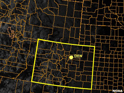
Late in the day on 23 October, the eastern half of Colorado was covered with stationary low upslope cloudiness and areas of fog and drizzle, associated with low-level easterly flow. This is shown in the GOES-8 1-km visible imagery where the laminar, stable top of the upslope cloud is evident.

Use of GOES Satellite Imagery to Differentiate Liquid and Ice Clouds (cont.)

Over the mountains to the west, deeper cloudiness of a different origin and air mass existed, moving with the westerly flow aloft and showing increased convective characteristics. This is shown in the loop of the GOES-10 10.7-µm IR imagery, and was associated with a weak wave aloft.

Reference

GOES 11-micrometer IR Window

Advantages
he best uses of the 11-micrometer IR window imagery for feature detection include:

• Detecting relatively cold cloud-top features associated with convection, cirriform, and mid-level cloud types
• Can be used in conjunction with cloud phase information obtained from shortwave infrared channels to help determine potential for icing
• Can be used in combination with shortwave infrared imagery for discriminating ice clouds at night. During daytime, it can be used to discriminate high clouds from snow and ice cover or in combination with shortwave IR and visible imagery.
• Can be used in conjunction with a shortwave infrared channel (between 3.5 and 4 micrometers) to detect water clouds at night

Limitations
The limitations of the 11-micrometer IR window channel for feature detection include:

• Distinguishing low clouds from relatively cold ground or water, a condition common during wintertime and at night
• Distinguishing between snow, ice cover, and adjacent frozen ground is very difficult
• Alone it cannot confirm the presence of supercooled water clouds, generally present between 0 and -15 degrees C

Use of GOES Satellite Imagery to Differentiate Liquid and Ice Clouds (cont.)

In addition, by examining the GOES 3.9-µm channel 2 imagery, we confirmed that the low-level stratiform cloud top was composed of primarily liquid by its relatively bright/warm appearance. Cloud droplets are efficient reflectors of incoming solar radiation at 3.9-µm, whereas ice is a poor reflector.

Over northwestern Colorado, the higher, more convective clouds moving eastward across the mountains contained more ice at their cloud tops. Note that some small areas of liquid cloud tops were apparent in the air mass above the inversion, but the larger, deeper entities were dominated by the ice phase at cloud top.

Use of GOES Satellite Imagery to Differentiate Liquid and Ice Clouds (cont.)

Later, as the deeper cloudiness moved eastward and over the laminar upslope cloudiness, the impact on precipitation type over the Colorado plains becomes evident. At 21UTC, observations indicated only fog and scattered freezing drizzle on the plains. By 01UTC on 24 October, light snow was beginning to show up over the Denver area, and by 02UTC was scattered over the northern Front Range of Colorado. This correlated well with the arrival of the deeper convective cloudiness.

These trends continued through 05UTC. By 06UTC mostly fog or no visibility obstructions were again dominant in the surface observations.

Use of GOES Satellite Imagery to Differentiate Liquid and Ice Clouds (cont.)

Until darkness set in, visible and infrared imagery revealed the eastward progression of the deeper cloudiness that was taking place. Between 22-23UTC, significant convective cloud elements were beginning to impact the urban corridor region just east of the foothills. This continued for a few hours, and by 05UTC on 24 October, the convective cloudiness was scattered from the Front Range eastward and was weakening over Colorado's northwestern quarter. Upslope cloudiness persisted during this time.

Use of GOES Satellite Imagery to Differentiate Liquid and Ice Clouds (cont.)

The GOES-8 10.7-µm IR imagery from 2330UTC 23 October to 0445UTC 24 October showed scattered higher colder cloud tops over northeastern Colorado progressing slowly eastward. Cloud-top temperatures reached -25 to -30°C over the weak convection, while the stratiform tops over northeastern Colorado remained at about -10°C.

Use of GOES Satellite Imagery to Differentiate Liquid and Ice Clouds (cont.)

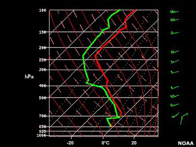
The 00UTC Denver (DEN) sounding, released several hours before the deeper cloudiness arrived, shows a deep moist layer from the surface to 400 hPa. It is especially saturated in and below the inversion at about 725 hPa. This inversion delineated the top of the upslope cloudiness from the moderate westerly flow aloft. Also notable is the slightly unstable lapse rate between about 650-500 hPa.

• DEN Sounding
• DEN Locator Map

Use of GOES Satellite Imagery to Differentiate Liquid and Ice Clouds (cont.)

Better spatial confirmation of the response to the seeder/feeder mechanism, as well as a more detailed picture of the structure of precipitation elements, is shown in the Doppler radar measurements from the FTG radar at the 0.5 degree elevation angle.

At approximately 22UTC, western Boulder and Larimer counties contained some cellular convective echoes to 25 dBz. By 00UTC, 20-25 dBz cells were beginning to progress onto the adjacent plains and showed some banded characteristics. At 01UTC, this progression correlated well with the appearance of scattered light snow in isolated surface observations.

The trend continued through 05UTC on the plains, with development of regions of reflectivity up to 30 dBz. By 07UTC, the cells were weakening and moving off towards the east.

Use of GOES Satellite Imagery to Differentiate Liquid and Ice Clouds (cont.)

This table shows the observed weather (when available) at the Jefferson County Airport (BJC) observation site in southeastern Boulder County along with the observed reflectivity over the site during the period of interest.

This confirms the development of light snow in the regions of enhanced 0.5 degree reflectivity. It implies that the deeper convective cloudiness was seeding the upslope cloudiness after 00UTC in this location, producing snowfall at the ground where only fog and patchy drizzle were associated with the upslope cloudiness prior to this time.

This small case study is a common high plains example where the seeder/feeder mechanism was active without a dry intervening layer between the seeder and feeder regions, the latter being the conventional seeder/feeder setup. In this case, the separation layer was simply an inversion that contained strong vertical wind shear.

Observations for Jefferson County Airport (BJC) 20-06UTC 23-24 October 2002
Time (UTC)	Weather	Reflectivity (dBz)
20	fog	<0
21	no weather	0-5
22	fog	<0
23	missing	<0
00	fog	0-5
01	lt. snow	5-10
02	missing	0-5
03	lt. snow shwrs.	10-20
04	lt. snow	10-15
05	missing	10-15
06	missing	15-20

Top of Page