Overview
Vorticity Minima and Anticomma Patterns
Season: Every day
Phenomena: Dry Circulation, Vorticity Minima, and Vertical Velocity
Tools: GOES water
vapour
Forecast Challenges:
- Identify and predict vorticity minima in order to predict areas of negative vorticity
advection
- Identify the related axes of maximum winds, shear zones, deformation zones, and air
masses
Vorticity minima signatures are every bit as common as vorticity maxima signatures. They indicate
areas of descending circulation and atmospheric forcing and can be used to diagnose dynamic
features such as the axis of maximum winds and deformation zones.
Note: All examples and conceptual models in this module are set in the northern
hemisphere. All graphics are oriented north to south with north on top.
Development of an Anticomma Pattern
The shape of the anticyclonic comma pattern reveals the location of the vorticity minimum. The
vorticity minimum is located at the point of inflection and is the center of the cloud rotation
in the atmospheric frame of reference. The shape of the concave inflow and convex outflow arcs
is related to both the relative intensity of the vorticity minimum and the length of time the
vorticity minimum has been acting on these arcs. The arcs become more concave or convex with
both vorticity minimum intensity and age.
The vorticity minimum (N) is the addition of both rotational vorticity (R) and horizontal wind
shear (S)—hereinafter simply referred to as shear. The following graphics illustrate the
concept. The size of the symbols indicates relative intensity.
Given pure rotation, this conceptual cloud line will evolve in symmetrical fashion. The
position of the vorticity minimum is at the center of the rotation, which is also the point
of inflection. The rotational vorticity is the sole component of vorticity.
There is no shear vorticity component.
With increased shear on the equatorial side of the rotation, the point of inflection and
the total vorticity is shifted towards that region of greater shear. As a result, the
concave arc is enhanced by stronger relative flow. The convex arc is not enhanced and is
created purely by the rotational component of the vorticity, which remains unchanged and
located at the center of the circle. The point of inflection is still the center of
rotation. It is also the location of the total vorticity minimum resulting from the sum
of the rotational and shear vorticities.
To summarize, this point of inflection is an anticyclonic outward cusp formed by the intersection of two anticyclonically
curved arcs directed toward the cusp. Typically, an anticyclonic outward cusp is created
by easterly speed shear that is equatorward of the cusp and marks the location of a
vorticity minimum.
With even greater shear on the equatorial side, the shear component of the vorticity
increases and there is more displacement. The total vorticity and point of inflection
shift toward the region of shear and away from the position of the rotational vorticity
centre. The concave arc is again enhanced with stronger relative flow.
If the shear is on the poleward side of the rotation, the same shifting of the point of
inflection takes place, again with the center of total vorticity shifting towards the
region of shear. In contrast, however, the convex arc in the location of the shear wind
maximum is enhanced. The concave arc is not enhanced and is created purely by the
rotational component of the vorticity, which remains unchanged and located at the center
of the circle. The vorticity minimum will be located within the moisture area as opposed
to the previous illustrations where it is located in the dry portion of the circulation.
Poleward shear comma clouds are common with the northeast trade winds in the tropics.
To summarize, this point of inflection is an anticyclonic inward cusp formed by the intersection of two anticyclonically
curved arcs directed toward the cusp. Typically, an anticyclonic inward cusp is created
by westerly speed shear that is poleward of the cusp and marks the location of a
vorticity minimum. This pattern is very common due to the prevailing westerly
circulations around the globe.
It's important to note that in these idealized examples the moisture extends right to the
vorticity centre. In the real atmosphere the moisture may dry out near the circulation centre,
especially as the circulation ages. As a result the actual point of inflection may be displaced
upstream from the apparent point of inflection revealed by the moisture patterns.
Morphology of an Anticomma Pattern
Roger Weldon originally identified the "comma" cloud pattern in the early 1980's. The anticomma
pattern is a mirror interpretation of that. Weldon showed correlations between the clouds,
streamlines, and absolute vorticity isopleths. Note that absolute vorticity isopleths are used
as an operational surrogate for system relative streamlines. Variation in cloud heights from
500-hPa and time differences between the analysis and the satellite data can lead to errors. The
centre of cloud rotation, as identified by the point of inflection, is the vorticity minimum to
a very close operational approximation.
Anticomma Dominated by Rotation and/or Equatorial Shear
The concave arc associated with the shear wind maximum defines this type of anticomma. The
anticomma head is downstream from the vorticity minimum. Negative vorticity advection will be
strongest in the anticomma head region.
Anticomma Dominated by Poleward Shear
The convex arc associated with the poleward wind maximum defines this type of anticomma. The
concave arc region is minimal and the point of inflection is within the moisture area. The
anticomma head is still downstream from the vorticity minimum.
Analysis
In the following interaction, take a look at the GOES water vapor loop, then analyze it for
vorticity minima, vorticity maxima, and the axes of maximum winds. After identifying these
features, compare your analysis to the one provided.
Satellite Loop
Look for vorticity minima in this GOES 4-km water vapour loop
After viewing the loop, click the Your Analysis tab
to
access the last image of the loop (1115 UTC) and mark the
location
of the vorticity minima, vorticity maxima, and
axes of maximum winds.
Your Analysis
The following exercise cannot be completed in Internet
Explorer 11 or older versions. Please use Microsoft Edge or other modern
browsers to complete this exercise.
Mark the location of the most prominent vorticity minima,
vorticity
maxima, and axes of maximum winds within the highlighted area.
Click the Done button to compare your analysis to the
"Expert's
Analysis".
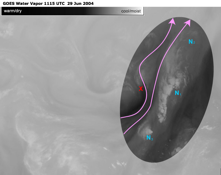
The most prominent anticomma formation is N1. The formation's
classic anticomma shape is comprised of convective cloud
that has smudged together.
There is an older vorticity minimum, N2, just barely visible
to the northeast and a younger one, N3, developing to the
southwest.
All are to the right of the flow looking downstream.
A vorticity maximum, X, is located to the left of the flow
looking downstream.
Interpretation
Let's take a closer look at this situation. First we'll look at the large scale atmospheric
circulations, then we'll focus on the main anticomma and vorticity minimum and finally, we'll
take a closer look at the moisture patterns associated with the series of anticommas.
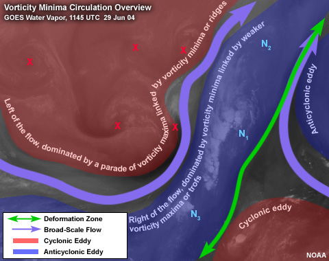
Circulation Overview
South of the main deformation zone, the flow is southerly. North of the deformation zone, the
general flow meanders from the west. There are eddies in both of these general flows. The
anticyclonic eddies are confined in the regions to the right of the general flow looking
downstream. The cyclonic eddies are confined in areas to the left of the general flow looking
downstream.
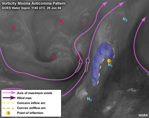
The Anticomma
Let's focus in on the largest anticomma. Some key points:
- The dominant vorticity minimum is to the right of the associated flow looking downstream.
- The classic anticomma shape happens to be comprised of convective cloud that has smudged
together.
- The vorticity minimum is the center of cloud rotation in the atmospheric frame of reference.
The vorticity center is certainly within the area of cloud rotation and most likely at the
point
of inflection. The concave arc is associated with the flow into the moisture area.
The convex arc is associated with the flow out of the moisture area.
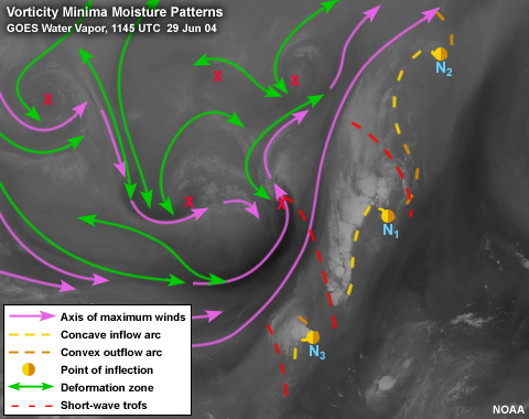
Moisture Patterns
From a moisture edge perspective, in order to identify the vorticity minimum, you are typically
interested in the concave or inflow arc of the anticyclonic pattern.
N1
This pattern happens to be comprised of well-developed convective cloud. The cirrus anvils of the
convection have blended together to reveal the circulations at the cirrus level that would
otherwise be difficult to discern. The convection is present as a result of upper divergence
upstream from the vorticity minimum.
This is good example of the anticomma with the moisture edge wrapping around the anticyclonic
center of rotation. The point of inflection separates the inflow concave arc and the outflow
convex moisture arc. The shape of the inflow concave arc is used to locate the vorticity
minimum. The best position of the vorticity minimum can be estimated by visualizing the oval
shaped circulation that best fits the inside moisture edge near the point of inflection. The
shape of this inflow arc is molded by the rotation. The vorticity centre is certainly within the
“best fit” oval and most likely at the point of inflection.
N2
The same principles apply to identifying this anticomma although the circulation is much drier
and more difficult to discern. Note the greater depth of the concave inflow arc. If the
vorticity minima are all of similar strengths (which is a good approximation since they are all
the result of the same relatively straight axis of maximum winds), then this circulation has
been acting on the concave inflow arc of N2 longer than either of the others. This implies that
the associated vorticity minimum is the oldest of the three and the most likely to be identified
correctly by NWP.
N3
Anticomma N3 can be identified solely by convection. In a similar discussion to the above, this
vorticity minimum is the youngest of the three and is the least likely to be well identified by
NWP.
Notice that the wavelength between the vorticity minima is quite uniform. This is because the
axis of maximum winds generating the vorticity minima is relatively straight and because of the
cyclical nature of short waves in the atmosphere.
Comparison with NWP
In this case, the NWP and observed vorticity minima correspond fairly well. The observed location
of the vorticity minimum is based on the point of inflection at the atmospheric level of the
moisture. This moisture level may not correspond exactly with the pressure level of the NWP
analysis (500 hPa in this case). This mismatch in level could result in a discrepancy between
the observed location of the vorticity minimum and the NWP position.
The NWP vorticity minimum corresponding to the observed N1 is very well placed, as would be
expected with such a well-organized anticomma pattern. The position and strength of the
circulation have been well integrated into this model run. Vorticity minima that have been
correctly analyzed by NWP in previous analyses are more likely to be correctly analyzed in the
current and future analyses. Thus older vorticity minima are more likely to be correctly
analyzed than new vorticity minima which are just spinning up.
The same is true with N2, a relatively older vorticity minimum. But as the system moves further
from the land area and data sensors used in model initialization, there is more likelihood that
features such as this will be lost. Here the blue highlight is the implied vorticity minimum
that must exist between the two analyzed maxima. The accuracy of the NWP positioning of the
vorticity minimum depends upon the amount and quality of the observational data in the area.,
Oceanic areas are typically data sparse so that the vorticity minimum over oceans can be
misplaced through a lack of data.
Using the satellite animation, N3 is placed near the leading edge of new convection. The model
inappropriately places the analyzed vorticity minimum upstream from the convection. The NWP
error in this case is best illustrated by the NWP vorticity maximum lobe which attempts to
include the two separate anti-commas evident on satellite imagery, into a single pattern. The
NWP fails to resolve the two separate and distinct real vorticity maximum centres and instead
creates a single vorticity maximum centrally located within an elongated vorticity maximum lobe.
This is most likely due to model resolution issues.
Implications
The correct placement of the vorticity minima is vital to the placement of related dynamic
features such as the axis of maximum winds and deformation zones. All of these dynamic features
must fit cohesively into the atmospheric puzzle. The correct placement of a vorticity minimum
might be the piece of the puzzle required to correctly identify and place other dynamic
features.
Here are some important attributes of vorticity minima to keep in mind when identifying them:
- Circulations around vorticity minimum are typically weak. As a result, numerical analyses of
the atmosphere often have difficulty in their placement and appropriate relative
intensities.
- Anticyclonic circulations tend to be rather dry. As a result, using cloud as a tracer for
the circulation is often not possible. Water vapour is typically the only reliable tracer
for anticyclonic circulations.
- Correctly identifying and locating vorticity minima can help better predict convection and
cloud patterns.
Example 1: Pure Rotation
Here are a few examples of vorticity minima. As is often true on the forecast desk, cases are not
always as straightforward as the conceptual models. These real-world cases may not be the best
examples of vorticity minima, but then, how often do you see any perfect examples at the desk?
Carefully examine the loop before doing the analysis. Be sure to compare your analysis to the
ones provided.
Satellite Loop
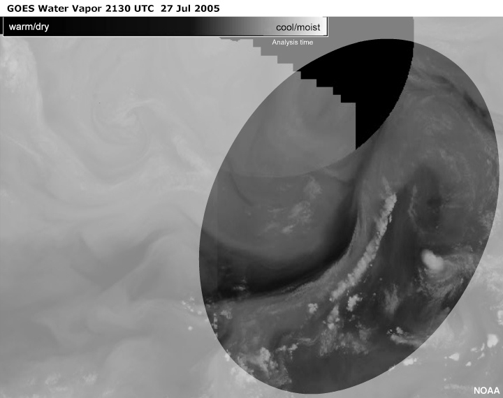
Focus in on the highlighted area of this GOES 4-km water vapour loop. Look for
the well-developed vorticity minimum with a a signature showing very little
shearing influences.
After viewing the loop, click the Your
Analysis tab to
access the last image of the loop (2130 UTC) and mark the
location
of the most prominent vorticity minimum, vorticity maximum,
and
axis of maximum winds.
Your Analysis
The following exercise cannot be completed in Internet Explorer 11
or older versions. Please use Microsoft Edge or other modern browsers to complete
this exercise.
Mark the location of the most prominent vorticity minimum,
vorticity
maxima, and axis of maximum winds within the highlighted
area.
Click the Done button to compare your analysis to the
"Expert's
Analysis".
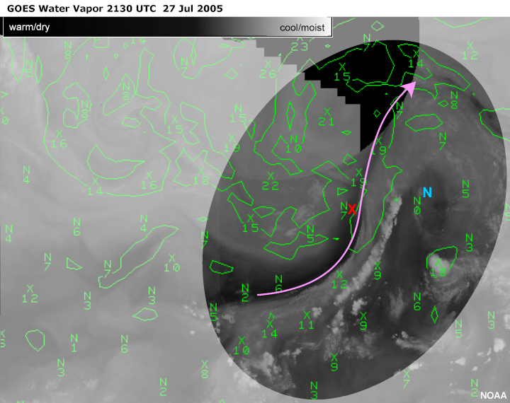
The most prominent anti-comma formation is well displaced to the
right of the axis of maximum winds. Shear influences are minimal and
the vorticity minimum is the result of rotation.
The GFS180 500-hPa absolute vorticity for 00-hr 0000 UTC 28 July,
which is a bit later in time than the satellite image, is in decent
agreement with the placement of the vorticity centres. The vorticity
maximum is downstream as anticipated. And also as expected, the
vorticity minimum is not as well placed.
Example 2: Equatorial Shear
Carefully examine the loop before doing the analysis. Be sure to compare your
analysis to the ones provided.
Satellite Loop
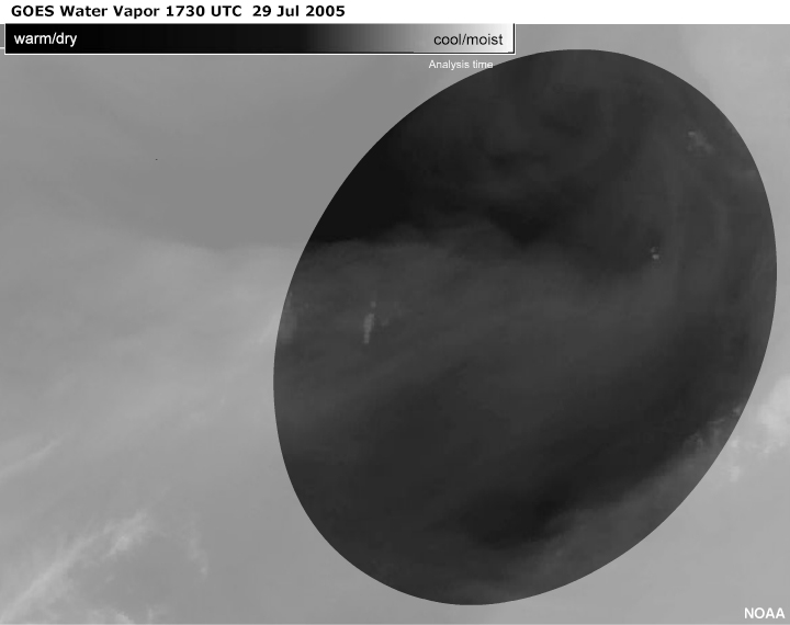
There is a subtle but fairly well-developed vorticity minimum in this GOES 4-km
water vapour loop. It is showing the signature of having equatorial shear.
After viewing the loop, click the Your
Analysis tab to
access the last image of the loop (1730 UTC) and mark the
location
of the most prominent vorticity minimum, vorticity maximum,
and
axis of maximum winds.
Your Analysis
The following exercise cannot be completed in Internet Explorer 11
or older versions. Please use Microsoft Edge or other modern browsers to complete
this exercise.
Mark the location of the most prominent vorticity minimum,
vorticity
maxima, and axis of maximum winds within the highlighted
area.
Click the Done button to compare your analysis to the
"Expert's
Analysis".
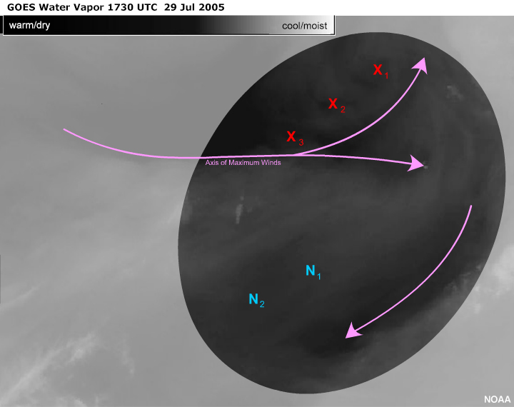
-
-
A northeasterly wind
maximum, as identified by darkening in the water
vapour image, is providing equatorial shear for the
vorticity minimum.
The darkening with the axis of maximum winds,
diverges with one stream wrapping around a set
of vorticity maxima. The other branch will wrap
around to the south and reinforce the northeasterly
winds.
Close the examination of the cyclonic shear reveals a
series of evenly spaced vorticity maxima.
Also, a classic large scale
bookend vortex pattern is revealed by the presence
of the deformation zone. Close examination reveals a
small vorticity maximum, X4, associated with the
northeasterly wind maximum.
N1 is the point of inflection evident due to
equatorial shear. N2 is a closed circulation
spinning in a northwestwardly direction. Without
enhancements, these signatures are very subtle.
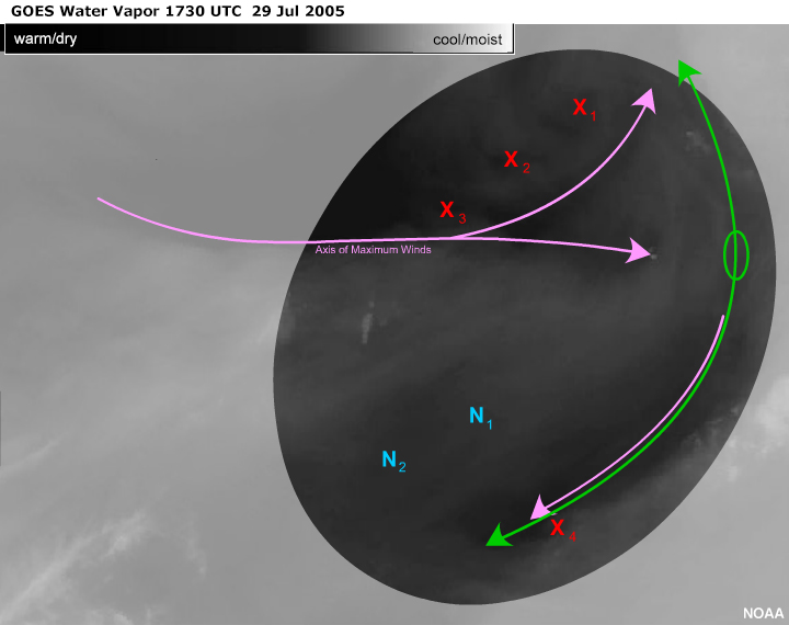
Looking at the GFS90 500-hPa
absolute vorticity for the 06-hr 1800 UTC 29 July, there
are acceptable correlations for all but X3. The model is
most likely not resolving the upper winds correctly. The
model pattern would imply a deeper trough with a
stronger wind maximum placed southeast of X3. This could
be due to the lack of data over the marine environment
and has implications for the onshore forecasts.
Example 3: Poleward Shear
Carefully examine the loop before doing the analysis. Be sure to compare your
analysis to the ones provided.
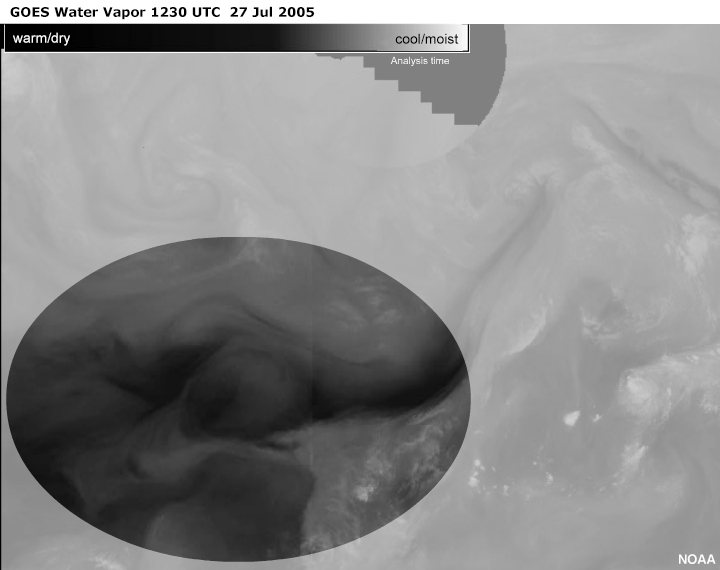
Satellite Loop
Within the highlighted area of this GOES 4-km water vapor loop, look for a
subtle vorticity minimum with the slight signature of having poleward shear.
After viewing the loop, click the Your
Analysis tab to
access the last image of the loop (1230 UTC) and mark the
location
of the most prominent vorticity minimum, vorticity maximum,
and
axis of maximum winds.
Your Analysis
The following exercise cannot be completed in Internet Explorer 11
or older versions. Please use Microsoft Edge or other modern browsers to complete
this exercise.
Mark the location of the most prominent vorticity minimum,
vorticity
maxima, and axis of maximum winds within the highlighted
area.
Click the Done button to compare your analysis to the
"Expert's
Analysis".
-
-
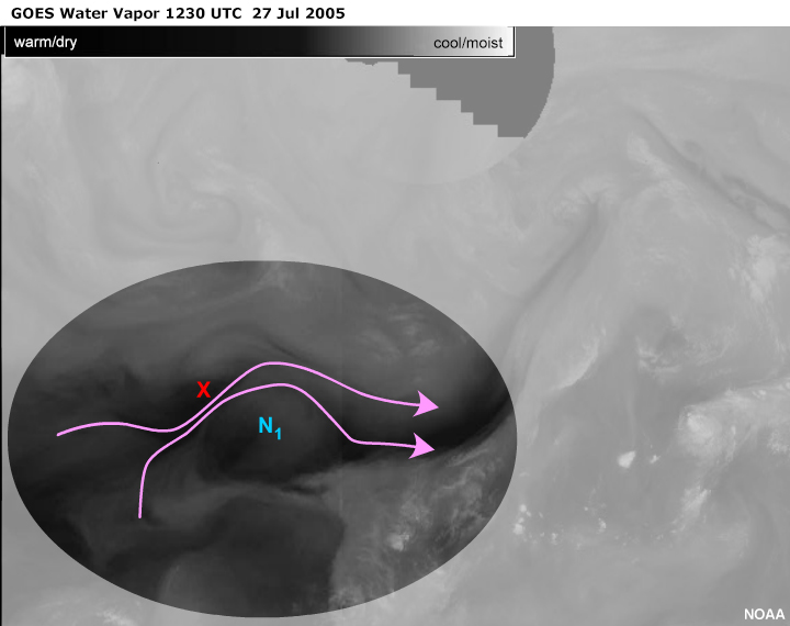
Within the highlighted area,
there's a westward flow meandering across a moderate
upper ridge. This flow is composed of two smaller scale
axes of maximum winds. Darkening on the water vapour
indicates the presence of a jet maximum between the
paired vorticity centres, X and N1.
The wind maximum is poleward of N1 resulting in the
characteristic though subtle moisture patterns as result
of poleward shear. The anticomma tail is quite dry
making this particular example challenging to identify.
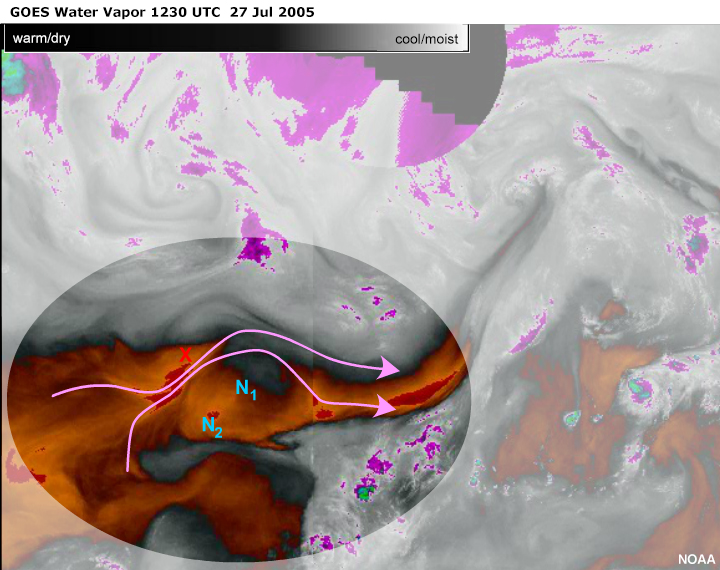
With enhanced water vapour
imagery, the contrast between moist and dry
mid-levels
stands out. The location of the jet maximum
separating
the paired vorticity centres is well marked. There
is
evidence of equatorial shear and a second vorticity
minimum, N2, at the point of inflection of the now
apparent anticomma head.
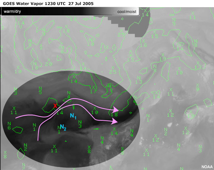
Looking at the GFS180
500-hPa
absolute vorticity for the 00-hr 0000 UTC 27 July,
there
is excellent agreement for the placement of the
vorticity maximum. As can be expected, the weaker
circulations of the vorticity minima are not well
resolved. The higher time and space resolution of
the
satellite imagery provides detail that could be
important in the predictive process.
This concludes Vorticity Minima and Anticomma Patterns,
please take a
few minutes
to
take the Quiz, and then
fill out our User
Survey.