Module Goal and Objectives
Module Goal
The goal of this training module is to help you increase your understanding of how and why coastally trapped wind reversals (CTWRs) occur. Such understanding, in turn, can help you more efficiently and accurately evaluate the synoptic and mesoscale conditions that might result in a CTWR.
Performance Objectives
At the end of the module you should be able to do the following things:
With regard to characteristics of CTWRs
- Describe how pressure, temperature, and wind change with passage of a coastally trapped wind reversal (CTWR)
- Recall how quickly CTWRs propagate up the U.S. West Coast
- Recall why SLP rises after passage of a CTWR
- Locate areas likely to experience CTWRs on a physical map of the world
- Recall the frequency of CTWRs along the California coast
- Explain why CTWRs are best explained as a Kelvin wave, rather than a gravity wave
With regard to the structure of CTWRs
- Describe how the MBL changes with passage of a CTWR
- Recognize how a cross-coast profile of the MBL changes during a CTWR
- Recognize a CTWR on a wind profiler record
- Recall the height at which wind first reverses direction as a CTWR propagates
- Recall the association of stratus formation with CTWRs
With regard to the synoptic evolution of CTWRs
- Describe how MSLP, 850mb heights, and 500mb heights depart from climatologic norms during a CTWR
- Describe how changes in MSLP and 850mb pressure force low-level offshore winds, and how this affects sensible weather along the coast
- Describe how variations in MSLP affect along-shore pressure gradients
With regard to the mesoscale evolution of CTWRs
- Recall how the synoptic setup forces the mesoscale offshore low
- Recall how the offshore low moves during a CTWR
- Describe how coastal mountains force ageostrophic flow
- Recall how coastal mountains contribute to warming of offshore winds
- Describe how and why a mesoscale high forms along the coast
- Recall the factors that cause northward propagation of the CTWR
With regard to forecasting CTWRs
- Recall the 3 best synoptic clues for forecasting a CTWR
- Recall where the offshore low forms with respect to the low-level offshore flow
- Recall where the stratus surge initiates with respect to the offshore low
- Describe the use and limitations of mesoscale NWP models in predicting CTWRs
Scenario
Scenario » 0200Z 22-May-99 (1900 PDT 21-May)
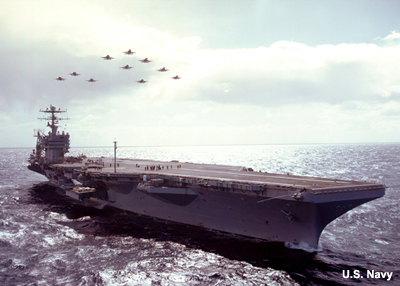
As the Leading Petty Officer and Flight Forecaster for the USS Abraham Lincoln, the last few days have not been very enjoyable. The carrier just spent two weeks in the Southern California Operations Area, just offshore of San Diego, conducting final qualifications for the F-14 Tomcat, F/A-18 Hornet, and S-3 Viking aircraft of the Airwing. Unfortunately, flying weather in SOCAL was miserable due to a strengthened marine layer producing fog and stratus. Two weeks in the Operations Area and we barely met the minimum number of required flight hours. Two weeks of having the Commanding Officer, Commander Air Group, and Air Boss complaining about lost flight training.
Scenario » Going Home
Now, we are heading north towards Point Conception on the way home to Bremerton, WA. We look forward to getting away from the influence of the Catalina Eddy. Tomorrow's Air Plan calls for a full day of launches and recoveries to make up for the lost flight training down south.
A Catalina Eddy forms when upper-level, large-scale flow off Point Conception interacts with the complex topography of the Southern California coastline. As air crosses the east-west oriented mountain ranges just east of Point Conception and descends to the ocean, the pressure on the air increases, causing it to warm dramatically. Consequently, a region of relatively low pressure develops in the lower atmosphere, with its center in the vicinity of Catalina Island. Counterclockwise circulation around this low pressure draws cool marine air and coastal stratus up the coast from the south, creating the eddy.
Catalina Eddy formation is accompanied by a southerly shift in coastal winds, a rapid increase in the depth of the marine layer, and a thickening of the coastal stratus. Catalina Eddies occur predominantly during the "stratus season," which is between April and September with a peak occurrence in June.
The effects of the Catalina Eddy on the weather over Southern California can be quite dramatic. When the Catalina Eddy is at its strongest, the depth of the low clouds may extend to 6000 feet. Usually, the increased thickness of the stratus clouds inhibits the typical morning/early afternoon burn off. Coastal temperatures will be several degrees cooler than the day before since cloud cover reduces the amount of surface heating from the sun.
Scenario » Synoptic Picture
The synoptic picture isn't unusual for this time of the year. A moderately strong surface high-pressure system is centered off the California — Oregon border with ridging extending into Idaho and Montana. I am particularly interested in the inverted trough at the surface that extends through California and north to the Oregon border. The interaction between these two systems will most likely be the dominant synoptic feature driving the flying weather this day. The inverted trough is progged to maintain its strength on the Eta forecast. The 850mb chart indicates weak troughing stacked above the surface with weak offshore ridging existing at 500 mb. Inland, the 500mb chart shows troughing extending from the northern tier to Baja California. This pattern aloft overall is progged to persist through tomorrow, with some weakening in the 500mb troughing over the northern Rockies.
Surface
850 mb
500 mb
An inverted trough is a trough in the pressure contours that has a different orientation with respect to the primary low pressure center than the conventional trough. Typically, the inverted trough extends northward from the low. The heat low of the desert southwestern region of the U.S. often includes an extension of low pressure northwestward along the elevated terrain of California and Nevada. This extension is an inverted trough.
Scenario » Surface Winds
The synoptic situation is forcing offshore winds along central and northern California, which has cleared out the marine layer. Surface winds from buoy and ship data are coast-parallel and out of the northwest.
I still don't see any problems with supporting today's flights. The models support winds from the north-northwest along the central California coast. Great-winds generally from the north to northwest means we can maintain Foxtrot Corpen. It also means that we can continue towards home and time with the family.
Direction of carrier into the wind + required to maintain enough winds over the bow to launch and recover aircraft.
Scenario » Good News
Time for the first round of flight briefs. The crews are happy to hear that they can expect CAT 1 conditions, in other words daytime Visual Flight Rules, or VFR. This is a welcome relief from the previous few weeks. The CO and Navigator welcome the news that winds support a northern track throughout the launch and recovery sequence.
| Altitude | Visibility | Distance from Clouds |
|---|---|---|
| Below 10,000 feet MSL Within controlled airspace Outside controlled airspace |
3 statute miles 1 statute mile |
500 feet below 1000 feet above 5000 feet horizontal Same as above or clear of clouds below 1200 feet AGL |
| At or above 10,000 feet MSL | 5 statute miles | 1000 feet below 1000 feet above 1 statute mile horizontal |
Scenario » 1400Z 22-May-99 (0700 PDT)
It is early morning. We rounded Point Conception in the night and are on our way north. Flight schedule begins just as soon as we pick up the northerly flow. Then we can steady on a launch — recovery course. My forecast calls for winds from the NNW at 15-20 knots, and no clouds given the developing offshore flow as we move north from Point Conception. Sea condition is not expected to pose any problems with a 2-4 foot swell from the WSW and 3-5 foot wind waves from the NW. Basically, Category 1 conditions. The CO, CAG, and Navigator are going to love this.
Scenario » First Sign of Trouble
First sign of trouble is when we don't pick up the northwest winds as expected. Winds are 3-7 knots and are unexpectedly southeasterly. Is it possible that the trough axis has moved off the coast? Though the winds don't look promising, at least the clouds are absent to maintain VFR conditions, though a bank of stratus is evident to the south and close enough to make me nervous.
Scenario » Turning Back
Now the problems really begin. Winds have definitely shifted and are now from the south-southeast, parallel to the coast. This morning's MM5 run progged winds from the SW at 5-10 knots. There is definitely something screwy going on.
In order to launch our first cycle of aircraft, we will have to reverse course to the south. This is not something that pleases anyone on the ship. Plan is to turn south just long enough to launch the first cycle, turn back to the north to regain lost ground and then, if necessary, turn back to the south to recover the first wave and launch the second.
Scenario » Model Forecast
I look ahead in the model run and my worst fears are realized. The forecast for 2100Z shows southeasterly winds at 15 to 20 knots. The model got it right, but just about 6 hours late!
Now, as we churn south seeking launch winds, we move into fog and low stratus, reducing visibility to barely above minimums. What was meant to be a perfect flying day has turned into the same morass of low visibility and ceilings hampering operations. To make matters worse, we have had to lose ground on our planned return cruise home.
Scenario » Fog and Stratus
The CAG and CO decide to cancel the first cycle of launches. I look at the latest imagery and notice that the fog and stratus (basically the strengthened marine layer) have moved north along the coast at a fairly rapid pace. We will need to get well north of San Francisco in order to conduct flight ops.
Scenario » Launch Conditions

Three hours of steaming north at full speed breaks us out into the clear and VFR levels again, but winds are still out of the south. Once again we are forced to reverse course to get launch winds. This time the launch sequence is successful.
Scenario » 20 Knots
Sometimes it just doesn't pay to be a weatherman! Just as we are setting up to recover the first cycle and launch the second, we are once again in the soup. Low ceilings and reduced visibility meet us as we move south. We are forced to speed north far enough to get better visibility and have enough sea room to negotiate the recovery. My only suggestion to the CO is to delay flying until the next day so we can outrun the fog and stratus. Data from the weather buoys tells us that north of the stratus, winds are 15 to 20 knots out of the northwest, but it seems the clouds are moving up the coast almost as fast as we are!
Obviously something is happening here on the mesoscale that the MM5 can't quite handle in terms of the timing. Whatever it is caused a surge in southeasterly surface winds, followed closely by low stratus and fog. It started late last night down by Point Conception, passed San Francisco by 0900, and reached Cape Mendocino by 1600. That's almost 20 knots!
Characteristics
Characteristics » Overview
Characteristics » Overview » What are coastally trapped wind reversals?
Coastally trapped wind reversals are events that occur along mountainous coastlines in which the coast-parallel winds tend to reverse direction from their climatologic norm to the opposite direction.
Because they were originally associated with the occasional surge of coastal stratus northward along the U.S. West Coast, they have also become known as stratus surges or southerly surges. However, they do occur along other coastlines, typically west coasts, where cold upwelling results in a marine boundary layer capped by a strong low-level inversion.
Though these events were first noted due to their stratus surge, it's actually a reversal of wind direction that characterizes these events. The wind reversal then propagates along the coast toward higher latitudes.
In the case of the U.S. West Coast, the wind reverses from its normal northerly direction to southerly. This wind reversal then propagates northward.
Characteristics » Overview » Satellite Example
This image shows a visible satellite image overlain with surface observation from offshore buoys. Notice the narrow tongue of marine stratus, which has moved up the coast to a place north of San Francisco. This stratus and the southerly winds typically extend offshore about 100 km.
To the north of the stratus, at Point Arena, winds are out of the north-northwest.
South of the leading edge of the clouds, winds switch to southeasterly, with velocities up to 20 knots.
From an operational perspective, the most crucial aspect here is the low stratus cloud cover often accompanied by fog. This stratus/fog development typically lags the wind reversal by an hour or two at any given location. Adding to your forecast challenge and aggravation, these events typically follow a clear day.
Characteristics » Climatology
Characteristics » Climatology » Global Locations
Coastally trapped wind reversals can occur along many mountainous coastlines around the world. The most likely locations include the west coasts of the U.S., Canada, South Africa, and Chile. All of these locations are characterized by cold upwelling of deep ocean water. This cold water favors the development of a marine boundary layer capped by a strong low-level inversion. This strong low-level inversion can then be forced by an appropriate synoptic scale pattern to initiate a coastally trapped wind reversal.
Characteristics » Climatology » Timing of Events
As this animation shows, events typically start propagating northward during the night, after daytime sea breezes dissipate. Obviously, if a forecaster relies only on visible imagery to spot the stratus surge, they may miss the first few hours of an event, during which the stratus can advance 100 km or more up the coast.
Along the U.S. West Coast, coastally trapped wind reversals typically occur in the warm months of the year, April through September. In Chile, similar events are reported to occur about once a week throughout the year.
Characteristics » Climatology » Frequency of Events
How often do they occur? Along the U.S. West Coast, events like this occur about 1 to 2 times per month in the summer. However, they do not explain the return of stratus following a clear spell on all occasions.
Characteristics » Climatology » Question
Question 1
On the image below:
- Use the white pen to mark three likely locations to find a coastally trapped wind reversal.
When you have finished, select Done.
Compare your answer to the answer below.

The U.S. West Coast experiences coastally trapped wind reversals 1 to 2 times per month in the summer.
In Chile, these events are reported to occur about once a week throughout the year.
Coastally trapped wind reversals were first documented in South Africa in 1977, by Adrian Gill.
Characteristics » Climatology » Summary
Coastally trapped wind reversals (CTWRs) are events where coast-parallel winds tend to reverse direction from their climatologic norm to the opposite direction. The wind reversal then propagates along the coast toward higher latitude.
CTWRs occur along mountainous coastlines, typically west coasts, where cold upwelling results in a marine boundary layer capped by a strong low-level inversion. On the U.S. West Coast, these events occur about 2 times per month in the summer.
CTWRs are frequently (though not always) associated with a surge of coastal stratus, thus they have also become known as stratus surges.
Coastally trapped wind reversals are important in the coastal region primarily due to (1) the rapid change from clear to cloudy conditions and (2) the rapid change in wind direction. The wind shift is from the climatolgical norm (northerly flow in the U.S.) to the opposite direction.
Characteristics » Observations and Structure
Characteristics » Observations and Structure » Composite Time Series at Different Buoys
So, what would you expect to see over the course of a coastally trapped wind reversal? This figure shows an 11-year composite of surface observations from 4 different weather buoys up and down the west coast. Each line represents an average of 14 to 28 events. The yellow line shows the time that the disturbance passes by any given buoy.
Notice the striking change in along-shore wind: from northerly, shown with negative values, to southerly, shown with positive values.
At the same time, the cross-coast wind shows only a small variation, and little or no indication of reversal. In general, the cross-coast component of wind is much weaker than the along-shore component, reflecting the fact that winds tend to parallel the coast.
Notice how the sea-level pressure falls to a minimum just before passage of the wind reversal, and then climbs for the next 24 hours or so. This increase of pressure reflects characteristic changes in the depth of the boundary layer.
Finally, note the temperature plot. Most of the lines show no change in temp AT THE SURFACE, which indicates that the boundary layer air mass does not change. The pressure change noted above consequently represents either changes in the depth of the cool, marine boundary layer or change in thermal properties above the boundary layer.
Characteristics » Observations and Structure » Vertical Structure
This figure shows time-height cross section of wind and virtual temperature as a wind reversal passes. The data come from a wind profiler located onshore at Fort Ord, near Monterey, California. In this plot, time moves forward from right to left.
Early in the time series we see easterly offshore winds and temperatures warmer than 20°C. Climatologically, this is well above the norm. As the wind reversal passes at 2200Z, a cool marine boundary layer develops while there was no such layer earlier, which suggests the flow of a cool, dense air mass in a gravity current.
This time series perspective inside of the Monterey Bay fails to depict the actual vertical structure of these wind reversals, which can be seen in the following cross sections constructed using aircraft observations.
Characteristics » Observations and Structure » Coast-parallel Structure
This figure shows a cross section parallel to the coast of potential temperature and along-coast wind speed. The light shading indicates southerly winds. The dark shading near the sea surface indicates stratus. The thin solid lines represent potential temperature.
Looking at the potential temperature, with the approach of the wind reversal we see the top of the inversion rising significantly, deepening the inversion layer and weakening the stratification. Meanwhile, the base of the inversion pretty much remains in place, with little change across the wind reversal. This fits well with the lack of a temperature change observed at the surface during wind reversals. At the same time, the sea level pressure goes up across the reversal due to the thickening of the inversion.
The light shaded region shows winds with a southerly along-shore component. Here we see that the wind first reverses direction aloft, well ahead of the leading edge of the wind reversal at the surface. The wind reversal correlates well with the thickening of the inversion.
Characteristics » Observations and Structure » Question
Question 2
Use the pull-down menu to choose the best answer.
The correct answers are highlighted above.
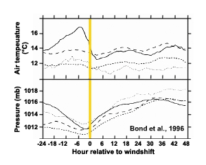
This composite plot from buoys along the California coast shows that surface temperature stays about the same across a CTWR, while SLP reaches a minimum just prior to the wind reversal.
Characteristics » Observations and Structure » Question
Question 3
Use the pull-down menu to choose the best answer.
The correct answers are highlighted above.
Since SLP rises after passage of a CTWR, the MBL must either cool or thicken. Offshore buoy data show no appreciable change in temperature during a CTWR, so the MBL must thicken to account for the change in SLP.
Characteristics » Observations and Structure » Propagation of Wind Reversals
This satellite loop shows an example of a northward-propagating wind reversal. You can clearly see the northward progression of both the stratus and the wind reversal. In this example, the reversal propagated up the coast at 10 meters per second, or roughly 20 knots. Meanwhile buoy data show winds of 15 knots. Note how temperatures for any given buoy stay nearly constant as the reversal passes. This tendency for propagation at speeds faster than the wind is common and suggests that these reversals are a disturbance and NOT JUST ADVECTION. This is important in forecasting these events as they can arrive much more quickly than the winds suggest.
As we will discuss later, these disturbances occur along mountainous coastlines. It turns out that a disturbance, or wave, in a fluid that is contained by a border along one side is referred to as a Kelvin wave. Thus, it appears that coastally trapped wind reversals are one type of naturally-occurring Kelvin wave.
In this case, we can see clearing well after passage, though this does not always happen. In fact, these events can occur with no clouds forming at all, though that is definitely not typical. Also note that in this post-reversal clear zone, the winds remain southerly and temperatures remain nearly constant.
In summary, this example very nicely shows the major elements that we have been discussing:
- The event is defined by a reversal of wind direction accompanied by formation of stratus
- This wind reversal propagates faster than the winds behind it and appears to happen with little or no change in surface temperature observed at buoys
- While clouds typically form along with the wind reversal, they may subsequently clear, or may not even form. It is the wind reversal that defines the event, not the clouds
A Kelvin wave is an internal wave in the atmosphere (or ocean) that is confined along a boundary such as a coastline due to the effects of the earth's rotation.
For coastally trapped wind reversals, the Kelvin wave is a gravity wave that occurs at the marine layer inversion and is trapped along the coastline due to coriolis turning of the wind toward the coastal mountain barrier.
Characteristics » Observations and Structure » Kelvin Wave vs. Gravity Wave
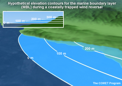
This illustration shows the height of the top of the MBL inversion near the coast during a CTWR. We can see that the MBL is deepest near the coast and slopes down to the west and northwest. The deep region near the coast is the zone of stratus and southerly winds. Since the deeper MBL results in a higher sea-level pressure, we can see that the southerly winds are a geostrophic response to the pressure gradient.
This structure is congruent with a Kelvin wave explanation for wind reversals, where a wave-like perturbation in the MBL lifts the top of the MBL. As a result of the lifting, stratus commonly forms and the winds initially blow down the pressure gradient and then eventually adjust geostrophically, as they switch from northerly to southerly.
Characteristics » Observations and Structure » Question
Question 4
Use the pull-down menu to choose the best answer.
CTWRs typically propagate faster than the wind behind them. This is one of the major arguments against a gravity current origin for CTWRs.
Characteristics » Observations and Structure » Question
Question 5
Use the pull-down menu to choose the best answer.
The correct answers are highlighted above.
As this figure shows, with passage of a CTWR, the top of the marine inversion rises, while the base stays about the same.

Characteristics » Observations and Structure » Summary
In a coastally trapped wind reversal, it is the wind reversal the actually defines the event. The clouds are not always present, or may have a much more complex structure than the disturbance itself. Therefore, we refer to these phenomena as coastally trapped wind reversals or coastally trapped disturbances, rather than stratus surges, because the stratus is a secondary feature.
These disturbances propagate northward faster than the wind, which suggests that they are not simply an advective process, but rather an internal, wave-like disturbance trapped against the coast (in other words, a Kelvin wave). The disturbance occurs within the inversion layer, above the surface.
High pressure in the cloudy region is due to an increased depth of the boundary layer or, more precisely, the inversion thickness.
Coastally trapped wind reversals are important in the coastal region primarily due to the rapid change from clear to cloudy conditions and the rapid change in wind direction.
Synoptic Scale Aspects
Synoptic Scale Aspects » Initial conditions
Synoptic Scale Aspects » Initial conditions » Introduction
These plots are a composite of several events, taken at the start of the event, centered on Buoy 13, near San Francisco. They illustrate the key aspects of the synoptic-scale structure that result in coastal wind reversals.
Synoptic Scale Aspects » Initial conditions » Sea Level Pressure
At sea level, we see the subtropical high pushed north of its climatological location into the Pacific Northwest, north of California. This is very characteristic of these types of events. Also note the warm thermal trough extending out toward the coast in an east-west direction. Normally this thermal trough is associated with the warm temperatures in the interior of California. The thermal trough tends to weaken the along-coast pressure gradient, or maybe even reverse it, so that we get higher pressures to the south and lower pressures to the north.
Synoptic Scale Aspects » Initial conditions » Questions
Question 6
Select the correct words to complete the sentence.
The correct answers are shown above.
Question 7
Use the pull-down menu to choose the best answer.
The correct answers are highlighted above.
The normal pressure gradient has higher pressures to the north. When the thermal trough extends offshore, we see lower pressures to the north, reversing the normal pressure gradient.
Synoptic Scale Aspects » Initial conditions » 850mb Height
At 850 mb we see a structure very similar to what we see at the surface, with ridging into the pacific northwest, and an axis of lower pressure extending out to the coast in southern California.
Synoptic Scale Aspects » Initial conditions » 850mb Wind
Associated with this intrusion of the ridge, we would expect to see northeasterly winds, and indeed that is the case, as shown here. So we have offshore flow just above the surface over northern and central California. This offshore flow is critical for the set up of coastally trapped wind reversals.
First, this offshore flow leads to clear conditions along the coast, which is atypical in and of itself.
Then, as this offshore wind comes across the mountains, we see adiabatic warming due to downslope flow in the lee of the coastal mountains.
Synoptic Scale Aspects » Initial conditions » 850mb Temperature
At 850 mb, we also see an extension of warm temperatures extending from the desert southwest out across the coast and over the ocean.
Synoptic Scale Aspects » Initial conditions » Questions
Question 8
Use the pull-down menu to choose the best answer.
The correct answers are highlighted above.
With a high-pressure center over the Pacific Northwest, anticyclonic flow favors offshore winds at 850 mb.
Question 9
Select the correct words to complete the sentence.
The correct answers are shown above.
Synoptic Scale Aspects » Initial conditions » 500mb Height
At 500 mb, we see the ridge axis just off the coast. So we have the surface high under the upper-level ridge axis. The extension of high pressure into the northwest is associated with increased subsidence downstream from the 500mb ridge axis. This sets up the low level offshore flow at 850 mb, which in turns sets up the coastally trapped wind reversal.
Synoptic Scale Aspects » 22-May-99: Surface
Synoptic Scale Aspects » 22-May-99: Surface » SLP 1200Z 21-May
The evolution of the conditions at the surface for our case, prior to the wind reversal and after, follow a pattern similar to that seen in many cases.
At 12Z on the 21st, we have a thermal trough up through central California, extending out toward the coast, with the subtropical high off to the southwest and weak ridging into the Pacific Northwest. This pattern is typical of the climatological summertime conditions.
Synoptic Scale Aspects » 22-May-99: Surface » SLP 1200Z 22-May
By 12Z on the 22nd, just prior to when the disturbance initiates, the trough extends offshore, the subtropical high has moved north, and the ridge is intruding into the Pacific Northwest.
At this point, even on the Eta model analysis, we can see a reversal of the pressure grad along the coast, with a low to the north near Monterey and a high to south in the California Bight. This gradient will favor southerly flow south of Monterey and northerly flow to the north of Monterey.
12 hours later, that reversal in the pressure gradient becomes more pronounced, with a well-defined nose of low pressure extending offshore from central California. Resulting ageostrophic winds will have a southerly direction from southern California to central California.
Offshore, we continue to see the subtropical high very far to the north with prominent ridging into the Pacific Northwest.
Synoptic Scale Aspects » 22-May-99: Surface » SLP 1200Z 23-May
Continuing into the disturbance, by this time (12Z on 23 May) the stratus has propagated north to about Cape Mendocino, though it doesn't show up in the Eta model. The trough axis extends toward the coast up into southern Oregon, and the subtropical high has pushed into southern Canada.
As the disturbance continues up the coast this day, the same pattern holds with ridging into the Pacific Northwest and a thermal trough extending offshore in northern California or southern Oregon. However, these features are starting to decay, and pressure gradients are starting to weaken.
Synoptic Scale Aspects » 22-May-99: Surface » SLP 1200Z 24-May
At 1200Z on the 24th, we see the synoptic structure decaying. The thermal low has weakened and moved very far north. The ridging is also weakening as the subtropical high is starting to rebuild to the southwest.
At the end of the sequence, we see the thermal low breaking down and the subtropical high retreating to the southwest. This sequence of the subtropical high building northward and into the Pacific Northwest followed by subsequent decay and retreat to the southwest is found in sea-level pressure evolution in composites of many cases.
Synoptic Scale Aspects » 22-May-99: 850 mb
Synoptic Scale Aspects » 22-May-99: 850 mb » 850 mb 1200Z 21-May
At 850 mb we see an evolution where initially coast parallel winds turn to become directed offshore to initiate a wind reversal.
At 1200Z on the 21st, prior to initiation of the disturbance, we see the subtropical high offshore to the south with the ridge axis extending into the Pacific Northwest. Winds are northerly across northern California, directed just slightly offshore and starting to clear out the stratus to set the stage for the coastally trapped disturbance.
Synoptic Scale Aspects » 22-May-99: 850 mb » 850 mb 1200Z 22-May
At 1200Z on the 22nd, the winds swing around more northeasterly as the subtropical high at 850 mb as well as the surface builds northward into the Pacific Northwest. This gives us stronger offshore flow, particularly across the northern and central California coast, with relatively warm temperatures across this region at 850 mb, suggesting warming with subsidence across the coastal mountain ranges.
We also see troughing at 850 mb from Cape Mendocino southeast across interior California, which is coincident with the warmest temperatures.
As the disturbance progresses through the day on 22 May, we see the thermal low strengthen and extend offshore. The 850mb ridge continues to build up into Canada with strong offshore flow all the way north into Washington, and the disturbance progresses up the coast during this time.
Synoptic Scale Aspects » 22-May-99: 850 mb » 850 mb 1200Z 23-May
By 1200Z on the 23rd the subtropical high is in retreat with the approach of a storm to the northwest. Offshore flow weakens during this time as the ridge in the Pacific Northwest weakens and the thermal low continues to move offshore.
Synoptic Scale Aspects » 22-May-99: 850 mb » 850 mb 1200Z 24-May
By 1200Z on the 24th, winds have turned to the northwest along the coast as the subtropical high retreats to the southwest and there is a return to typical climatological conditions with even more pronounced with northwesterly winds all along the coast by later on the 24th.
This evolution is similar to synoptic composites of other wind reversals and shows that the wind reversal is directly associated with the period of pronounced offshore flow at 850 mb. The wind reversal initiates as this offshore flow develops to the north and then it stops and decays as the offshore flow returns to typical northwesterly flow.
Synoptic Scale Aspects » 22-May-99: 500 mb
Synoptic Scale Aspects » 22-May-99: 500 mb » 500 mb 1200Z 21-May
Now let's look at the evolution of the 500mb heights and vorticity starting on 21 May. The 500mb ridge axis extends northward along the coast, but is located offshore. This is consistent with the composite evolution of many wind reversals 24-36 hours prior to the event. In this particular case, we also see a well defined closed low aloft over southern California. This results in northerly flow aloft over California at this time.
These conditions lead to subsidence and associated drying at low levels, which tends to clear out the coastal status in this region.
Synoptic Scale Aspects » 22-May-99: 500 mb » 500 mb 1200Z 22-May
24 hours later, at 1200Z on May 22, the 500mb ridge moves into the Pacific Northwest. The disturbance at low levels has started by this time, which started as the closed low migrated slightly to the northeast and northeasterly flow aloft developed.
Synoptic Scale Aspects » 22-May-99: 500 mb » 500 mb 1200Z 23-May
At 1200Z on the 23rd, the 500mb ridge axis migrates down the coast, weakens, and becomes ill-defined, while the closed low migrates eastward. The low-level disturbance weakens just beyond this time period.
Synoptic Scale Aspects » 22-May-99: 500 mb » 500 mb 1200Z 24-May
By 1200Z on the 24th we're starting to see the approach of a deeper trough offshore. By now the disturbance is completely over at the surface. Satellite imagery shows the stratus has made it about as far north as Cape Mendocino.
Overall, we see a progression aloft that starts with the 500mb ridge initially offshore. Then the ridge builds and moves into the Pacific Northwest as the disturbance is initiated in the low levels. Subsequently, the ridge weakens and moves east as the disturbance proceeds in the low levels. This upper-level evolution is very consistent with the synoptic evolution determined from composites of many cases.
Synoptic Scale Aspects » Conclusions
Synoptic Scale Aspects » Conclusions » Conclusions
Reviewing the synoptic scale surface feature, there are a couple of features that are important to note:
The disturbance essentially represents down-gradient flow from high pressure in southern California to low pressure to the north.
This ageostrophic flow northward along the coast is due to terrain blocking of surface winds by coastal mountains, in which the onshore flow is blocked by topography, and consequently turns toward lower pressure, which is located to the north.
Note that this ageostrophic response tells us why the wind reverses, but not why the disturbance propagates.
The wind reversal propagates northward much faster than the thermal trough, suggesting that there is a forced response associated with the disturbance. This forced response perturbs the marine boundary layer, lifting the top of the capping inversion and propagating northward as a Kelvin wave.
The synoptic scale is forcing a coastal low at a particular point, and even though that coastal low may drift northward, it tends to remain relatively fixed over the time period in which the disturbance propagates rapidly northward.
Synoptic Scale Aspects » Conclusions » 22-May-99
Here we see a satellite image from the last case taken at 1800Z on May 22nd. The image is overlain with sea level pressure and 850mb winds. At this time the disturbance was in full swing and the stratus had propagated to a point just north of San Francisco.
The reversed pressure gradient extends from the California bight region up the extension of the trough over the coast. This coincides with northern extent of the stratus, which marks the leading edge of the disturbance at the surface.
We see the offshore flow at 850 mb over northern California, which leads to adiabatic warming over the coast, tending to lower sea level pressure out ahead of the disturbance.
There are cases where this synoptic-scale setup persists, just like this, and we see no northward movement of the stratus. However, in this case the stratus continues to propagate northward along the coast, much faster than the synoptic features.
Mesoscale evolution
Mesoscale evolution » SLP
Mesoscale evolution » SLP » SLP Evolution
If we look the mesoscale sea level pressure pattern associated with one of these disturbances, we can infer relationship between the synoptic scale evolution and the structure of the perturbed marine boundary layer thickness that produces the coastal high pressure associated with the disturbance.
Mesoscale evolution » SLP » SLP 0000Z 10-Jun-94
Prior to the disturbance, we see low pressure in the California Bight region and increasing pressure north along the coast. This is consistent with the boundary layer inversion sloping down toward the coast, which is the climatological structure.
Mesoscale evolution » SLP » SLP 0600Z 10-Jun-94
By 6 hours later, we see an axis of lower pressure extending offshore just north of Point Conception. This region of low pressure occurs in the region of strongest offshore flow above the boundary layer and marks the initiation of the disturbance.
Mesoscale evolution » SLP » SLP 1200Z 10-Jun-94
As time progresses, we see the axis of low pressure along the coast has moved north to cross the coast near Monterey Bay. However, the offshore low remains relatively fixed at a location just north of the California Bight.
An axis of high pressure lies over Point Conception. This axis of high pressure mirrors what we see in satellite imagery and marks the disturbance and the stratus surge. The high pressure represents the deeper marine boundary layer associated with the disturbance.
Mesoscale evolution » SLP » SLP 1800Z 10-Jun-94
Another 6 hours later, we see the nose of high pressure right along the coast and a closed low offshore. The region of high pressure is propagating up the coast and is associated with southerly winds and stratus.
The low pressure is in about the same position as it was initially forced, just north of Point Conception; it hasn't really moved. This lack of movement reflects the tendency for the synoptic scale to evolve slowly. The strongest offshore flow is occurring in this region, forcing the low to form. The disturbance propagates northward under this offshore flow, leaving behind the coastal low that initiated the disturbance.
Mesoscale evolution » SLP » Question
Question 10
As the CTWR evolves, the center of the mesoscale offshore low ______. Choose the best answer.
The correct answer is e) "remains roughly stationary"
Because the mesoscale offshore low is forced by the synoptic offshore flow, it only moves as the synoptic situation evolves. Since the synoptic situation evolves slowly, the mesoscale offshore low remains roughly stationary through the life of the CTWR.
Mesoscale evolution » Temperature
Mesoscale evolution » Temperature » Temperature
The formation of the mesoscale coastal low that initiates the disturbance is due to localized warming along the coast. This can be seen in this comparison of soundings from Monterey. We see relatively cool temperatures in the initial sounding, to the left, and warming in the lower atmosphere 24 hours later, mostly below 850 mb.
But what causes the warming? If we look at winds, at the initial time we see relatively strong, low-level northeasterly winds. These winds cause the temperatures to rise in the low levels, which forms the low that initiates the disturbance. The region of strongest offshore flow marks the region of greatest warming and largest pressure falls along the coast. By the time the disturbance is under way, shown on the right, the forcing has weakened and we no longer see the northeasterly flow.
In this particular case, the low level warming is due almost entirely to advection of warm air offshore, though in some cases, there is a mix of advection and adiabatic warming.
Mesoscale evolution » Temperature » Question
Question 11
Formation of the offshore low is forced by _______ at low levels. Choose the best answer.
The correct answer is c) "warm, offshore flow"
Warm, dry, offshore flow forces the offshore low. Southerly flow would be very similar to the air it displaces, and cool, dry, offshore flow would not lower SLP.
Mesoscale evolution » Model Simulations
Mesoscale evolution » Model Simulations » Model Simulations
Horizontal cross sections at a height of 300 m above sea level. The coastal mountains lie along the right side of each cross section. Contour lines show potential temperature (contour interval = 2 K). Maximum wind vectors are approximately 14 m/s. The position of the imposed offshore flow is indicated on the far right.
The tendency for offshore flow to produce localized warming and a coastal low are characteristic synoptic-scale aspects of a disturbance. What we want to try to understand is how those synoptic features actually force this low pressure to occur along the coast, which then initiates a propagating wind reversal.
Shown here is a simplified model, which starts with strictly along-coast flow at inception. We then perturb this flow by blowing winds across the coast, as shown to the far right, and let the atmosphere evolve.
At one day into the simulation (far left) we start to develop a region of low pressure right at the axis of the strongest offshore flow. Winds are deflected away from the coast upstream of the low, and then around and toward the coast downstream of the low.
Mesoscale evolution » Model Simulations » Page 4-3-2
Coastal mountains block the winds flowing toward the coast. The blocked winds slow down, then respond ageostrophically, turning north toward the low pressure. We see this response about 1.5 days into the simulation with the narrow zone of southerly flow right along the mountains. We also see that the low pressure is still located right at the point of strongest offshore flow at this time.
Mesoscale evolution » Model Simulations » Day 2
At day 2, as the disturbance continues to evolve, and we see the axis of low pressure building and extending offshore and the wind reversal propagating north right along the coast, underneath the region of strongest offshore flow.
The pressure distribution looks very much like what we see in the observations with a narrow zone of high pressure right along the coast and a pressure gradient falling off to the north and west. This pattern reflects our forced Kelvin wave, with this feature now propagating up the coast.
Mesoscale evolution » Model Simulations » Question
Question 12
Select those factors that contribute to the northward propagation of the wind reversal. Choose all that apply.
All 3 choices are correct.
A mountainous coastline provides a barrier for terrain blocking. When airflow slows down while ascending slopes, it turns ageostrophically toward lower pressure. This process leads to southerly winds.
A strong inversion capping the MBL contributes to terrain blocking by increasing the wind speed required to overcome the coastal mountains. The higher the static stability of the atmosphere, the more likely terrain blocking becomes.
Strong, warm offshore flow is required to generate the mesoscale offshore low-pressure center. Flow around this low-pressure center is turned geostrophically toward the mountains, setting up terrain blocking.
Mesoscale evolution » Mesoscale Evolution
Mesoscale evolution » Mesoscale Evolution » Mesoscale Evolution
This graphic summarizes the model result and shows the evolution of a coastally trapped wind reversal.
Mesoscale evolution » Mesoscale Evolution » Preconditions
At our start time, t0, we see the climatologic norm with high pressure offshore, low pressure inland, and strong along-coast flow out of the north. The corresponding cross section shows a marine layer inversion sloping down into the coastal mountains.
Mesoscale evolution » Mesoscale Evolution » Initiation
At the next time step, t1, we initiate the zone of offshore flow. That offshore flow sets up the coastal low. The northerly surface flow gets perturbed around the low and turned in toward the coast around the south end of the low.
Mesoscale evolution » Mesoscale Evolution » Propagation
At the last time step, t2, the coastal mountains block the onshore flow, so it turns north toward the low, setting up the disturbance that propagates northward. The coastal low stays under the region of strongest offshore flow while the wind reversal and the coastal high propagate northward. The bottom cross section shows the inversion sloping down to the coastal low, then sloping back up to the coastal mountains, which reflects our coastally trapped disturbance.
Mesoscale evolution » Mesoscale Evolution » Question
Question 13
The offshore low acts to _____. Choose the best answer.
The correct answer is c. Coast-parallel winds from the northwest turn geostrophically when they encounter the offshore low, toward the coast, where they encounter the coastal mountains.
Question 14
Coastal mountains act to promote CTWRs by _____. Choose all that apply.
The correct answers are a and b.
The blocking of onshore flow by the coastal mountains forces that flow to turn northward, creating the CTWR. Downslope adiabatic warming of the offshore winds help clear out the MBL and leads to the formation of the offshore low.
The coastal mountains are not involved with the development of the subtropical high. The stability of the MBL and the strength of its capping inversion results from low-level cooling due to cool sea surface temperatures. These low sea surface temperatures result from upwelling that is common along west coasts.
Mesoscale evolution » Summary
Starting with synoptically-forced, offshore flow at 850 mb, we develop a region of low pressure right at the axis of the strongest offshore flow. Winds are deflected away from the coast upstream of the low, and then around and toward the coast downstream of the low.
Coastal mountains block the winds flowing toward the coast. The blocked winds slow down, then respond ageostrophically, turning north toward the low pressure. The low pressure is still located right at the point of strongest offshore flow.
As the disturbance continues to evolve, we see the axis of low pressure building and extending offshore and the wind reversal propagating north right along the coast, underneath the region of strongest offshore flow. The pressure distribution has a narrow zone of high pressure right along the coast and a pressure gradient falling off to the north and west. This pattern reflects our forced Kelvin wave, with this feature now propagating up the coast.
Forecasting
Forecasting » Overview
Forecasting » Overview » Overview
To forecast a coastally trapped wind reversal, there are a few things to note and watch for:
- For the synoptic set-up, watch for the intrusion of the subtropical high into the Pacific Northwest (for U.S. West Coast events), the extension of the thermal low over the coast, and the development of offshore directed winds at about the 850mb level of the atmosphere.
- Watch for where strongest offshore flow is. That will initiate the coastal low. The synoptic scale models should give reasonably good guidance on this location.
- Once the position of the coastal low is known, we should see the stratus surge develop to the south. Monitor buoy pressures to see if the pressure gradient reverses. That stratus surge may then propagate north, past the coastal low.
Forecasting » Overview » Question
Question 15
Select the 3 best synoptic clues for forecasting a CTWR. Choose all that apply.
The correct answers are a, b and e.
Low-level offshore winds are required to develop the offshore low. The extension of the thermal low over the coast reverses the normal along-shore pressure gradient, leading to northward propagation of the CTWR.Intrusion of the subtropical high into the Pacific Northwest sets up the low-level offshore flow.
Prior to a CTWR, the 500mb ridge typically amplifies, rather than flattens. Prior to a CTWR, 850mb winds intensify, but the flow is offshore, not southerly. Thickening of the marine boundary layer is a mesoscale response to synoptic forcing.
Forecasting » Overview » Question
Question 16
The offshore low typically forms where the ______ crosses the coast. Choose the best answer.
The correct answer is b.
The position of synoptic features including the 500mb ridge, subtropical high, and thermal low determine the location of the strongest offshore flow. This offshore flow most directly determines the position of the offshore low, so (b) is the best answer.
Forecasting » Using Mesoscale NWP Models
Forecasting » Using Mesoscale NWP Models » Mesoscale NWP Models
How well do mesoscale models predict coastally trapped wind reversals?
The synoptic scale forcing is handled quite well by mesoscale models. These models typically show us the inland intrusion of the subtropical high, the offshore extension of the thermal low, and the development of offshore winds.
In addition, mesoscale models can sometimes depict coastal wind reversals and changes in the depth of the marine boundary layer. However, mesoscale models tend to overemphasize sea breezes and diurnal forcing, which can mask some of the features of coastally trapped wind reversals and make those features hard to see.
However, do not expect mesoscale models to depict the exact timing and location of this type of disturbance. The details of the wind reversal are not handled well and the clouds themselves are handled more poorly still.
Forecasting » Using Mesoscale NWP Models » Disturbance Missing
Here is an example of a mesoscale model, the MM5, run for the 22 May case we looked at earlier.
This figure shows a 3-hour forecast of surface winds overlain on the satellite image. We can see that the disturbance is in full swing with stratus reaching nearly to San Francisco. The model predicted southwesterly flow in the clouds, at a time when observations indicated southeasterly flow, so the model is missing the disturbance at this point.
Forecasting » Using Mesoscale NWP Models » Reversal Mis-located
Three hours later, the disturbance has moved up the coast. The mesoscale model has been able to turn the winds into a more coast parallel direction, and therefore, is starting to see the disturbance. However, the model shows the wind reversal occurring somewhere south of Monterey, while the leading edge of the disturbance is well north of San Francisco.
Forecasting » Using Mesoscale NWP Models » Reversal Mis-timed
Another 3 hours later, at 2100Z, the clouds show the disturbance continuing to propagate north. The model predicts southerly winds up into Monterey Bay and shows the disturbance propagating up the coast. However, while the model recognizes the coastally trapped wind reversal, it is still places the disturbance too far to the south. The model is missing on the timing; it started late and cannot seem to catch up.
Forecasting » 22-May-99
Forecasting » 22-May-99 » Sea Level Pressure and Wind
Looking now at a loop of sea level pressure and wind from the MM5.
In the analysis, we see a weak coastal low starting to perturb the along-coast flow.
Forecasting » 22-May-99 » 3-hr Forecast
3 hours into the model run, the low pressure offshore strengthens. As a result, the model starts to turn the winds in toward the coast.
Forecasting » 22-May-99 » 6-hr Forecast
Six hours into the forecast period, the offshore low continues to build and we start to see coastal southerlies. At this time, the model progs the leading edge of the dusturbance along the northern side of Monterey Bay, near Santa Cruz. In reality, the stratus lies well north of San Francisco at this time
Forecasting » 22-May-99 » 9-hr Forecast
As the model proceeds, it propagates the disturbance up the coast. The model now locates the disturbance about half way between Monterey Bay and San Francisco.
Forecasting » 22-May-99 » 12-hr Forecast
Here at 12 hours, the model-defined disturbance extends up to about San Francisco, with low pressure offshore and high pressure in the disturbance.
Forecasting » 22-May-99 » 15-hr Forecast
The 15-hour forecast shows the disturbance continuing to propagate northward. However, it also shows a surge into interior California, which was not observed.
Overall, with mesoscale models we can see that some of the details are wrong and the timing is off. And though it isn't shown here, if we were to look at cross sections, we would find that the marine boundary layer structure is oftentimes not particularly well handled, though it can capture bulging of the MBL along the coast.
Sometimes numerical models can provide some useful guidance. They can simulate some of the features of a disturbance, but they are very sensitive to the timing of the synoptic scale forcing and to the details of the marine boundary layer structure that they start with. In some weaker cases the model may completely miss forecasting any of the salient features that typically occur.
Forecasting » 22-May-99 » Question
Question 17
Mesoscale NWP models will best depict the ______. Choose the best answer.
The correct answer is a.
NWP models, even mesoscale ones, have their greatest difficulties with clouds and precipitation. And as the example showed, mesoscale models may capture the general phenomena of a CTWR, but not the exact timing and details. On the other hand, mesoscale models will most likely do a very good job with the synoptic forcing, including the offshore winds that result. So the best answer is A.
Forecasting » Return to Normal
As the synoptic conditions return to more zonal flow aloft and northwesterly flow at 850 mb, the disturbance tends to end because there is no low-level offshore flow to maintain the coastal low. Oftentimes the clouds are left in place along with a deeper marine boundary layer.
We then have climatological conditions and a deep marine boundary layer along the coast until the next trough comes through to clear things out.
Summary
Characteristics
Coastally trapped wind reversals (CTWRs) are events where coast-parallel winds tend to reverse direction from their climatologic norm to the opposite direction. The wind reversal then propagates along the coast toward higher latitude.
CTWRs occur along mountainous coastlines, typically west coasts, where cold upwelling results in a marine boundary layer capped by a strong low-level inversion. On the U.S. West Coast, these events occur about 2 times per month in the summer.
CTWRs are frequently (though not always) associated with a surge of coastal stratus, thus they have also become known as stratus surges.
Coastally trapped wind reversals are important in the coastal region primarily due to the rapid change from clear to cloudy conditions and the rapid change in wind direction from the typical northerly flow to a southerly flow.
Structure
It is the wind reversal that actually defines the event. The clouds are not always present, or they may have a much more complex structure than the disturbance itself.
These disturbances propagate northward faster than the wind, which suggests that they are not simply an advective process, but rather an internal wave-like disturbance trapped against the coast (i.e., a Kelvin wave). The disturbance occurs within the inversion layer, above the surface.
High pressure in the cloudy region is due to an increased depth of the boundary layer or, more precisely, the inversion thickness. Across a CTWR, the top of the inversion capping the MBL rises significantly, deepening the inversion layer and weakening the stratification. Meanwhile, the base of the inversion pretty much remains in place, with little change.
All of these changes occur very low in the atmosphere, typically below 850 mb, within the marine boundary layer and its capping inversion.
Synoptic evolution
At the time of initiation we see a well-defined 500mb ridge offshore with troughing over the intermountain west. The subtropical high has pushed into the Pacific Northwest, and the resulting offshore flow has cleared out the coastal stratus. As the subtropical high moves eastward, offshore flow intensifies and the thermal trough moves out across the coast. This sequence initiates the disturbance in the low levels.
As the disturbance proceeds, we see the 500mb ridge moves into the coast. Associated with that movement, the 850mb ridge axis extends well into the Pacific Northwest, with a similar pattern in the sea level pressure.
24 hours into the disturbance, the 500mb ridge axis crosses the coast and weakens. Consequently, we see we see a relaxation of the 850mb ridge and weaker offshore flow. The disturbance starts to weaken at the surface as well.
After 48 hours we see patterns very much like what we started with 48 hours before the disturbance, with zonal flow aloft and the low-level ridges retreating offshore. The disturbance at the low levels is essentially over at this point.
Mesoscale evolution
Starting with synoptically-forced offshore flow at 850 mb, we develop a region of low pressure right at the axis of the strongest offshore flow. Winds are deflected away from the coast upstream of the low, and then around and toward the coast downstream of the low.
Coastal mountains block the winds flowing toward the coast. The blocked winds slow down, then respond ageostrophically, turning north toward the low pressure. The low pressure is still located right at the point of strongest offshore flow.
As the disturbance continues to evolve, we see the axis of low pressure building and extending offshore and the wind reversal propagating north right along the coast, underneath the region of strongest offshore flow. The pressure distribution has a narrow zone of high pressure right along the coast and a pressure gradient falling off to the north and west. This pattern reflects our forced Kelvin wave, with this feature now propagating up the coast.
Forecasting
To forecast a coastally trapped wind reversal, there are a few things to note and watch for:
- For the synoptic set up, watch for the intrusion of the subtropical high into the Pacific Northwest, the extension of the thermal low over the coast, and the development of offshore winds in the low levels of the atmosphere.
- Watch for where the strongest offshore flow is. That will initiate the coastal low. The synoptic scale models should give reasonably good guidance on this location.
- Once the position of the coastal low is known, we should see the stratus surge develop to the south. That stratus surge may then propagate north, past the coastal low.
Using mesoscale NWP models:
- The synoptic scale forcing is handled quite well by mesoscale models. These models typically show us the inland intrusion of the subtropical high, the offshore extension of the thermal low, and the development of offshore winds.
- Mesoscale models can sometimes depict coastal wind reversals and changes in the depth of the marine boundary layer. However, mesoscale models tend to overemphasize sea breezes and diurnal forcing, which can mask some of the features of coastally trapped wind reversals and make those features hard to see.
- Do not expect mesoscale models to depict the exact timing and location of this type of disturbance. The details of the wind reversal are not handled well, and the clouds themselves are handled more poorly still.
Bibliography
Bond, N. A., C. F. Mass, and J. E. Overland, 1996: Coastally trapped wind reversals along the United States west coast during the warm season. Part I: Climatology and temporal evolution. Monthly Weather Review, 124, 430-445.
Garreaud, R.D., J.A. Rutllant, and H. Fuenzalida, 2002: Coastal Lows along the Subtropical West Coast of South America: Mean Structure and Evolution. Monthly Weather Review, 130, 75-88.
Gill, A.E., 1977: Coastally trapped waves in the atmosphere. Quarterly Journal of the Royal Meteorology Society, 103, 431-440.
Mass, C. F., and N. A. Bond, 1996: Coastally trapped wind reversals along the United States west coast during the warm season. Part II: Synoptic evolution. Monthly Weather Review, 124, 446-461.
Nuss, W. A., J. M. Bane, W. T. Thompson, T. Holt, C. E. Dorman, F. M. Ralph, R. Rotunno, J. B. Klemp, W. C. Skamarock, R. M. Samelson, A. M. Rogerson, C. Reason, and P. Jackson, 2000: Coastally trapped wind reversals: Progress toward understanding. Bulletin of the American Meteorological Society, 81, 719-744.
Ralph, F. M., P. J. Neiman, P. O. G. Persson, J. M. Bane, M. L. Cancillo, J. M. Wilczak, and W. Nuss, 2000: Kelvin waves and internal bores in the marine boundary layer inversion and their relationship to coastally trapped wind reversals. Monthly Weather Review, 128, 283-300.
Ralph, F. M., L. Armi, J. M. Bane, C. Dorman, W. D. Neff, P. J. Neiman, W. Nuss, and P. O. G. Persson, 1998: Observations and analysis of the 10-11 June 1994 coastally trapped disturbance. Monthly Weather Review, 126, 2435-2465.
Skamarock, W. C., R. Rotunno, and J. B. Klemp 1999: Models of coastally trapped disturbances. Journal of the Atmospheric Sciences, 56, 3349-3365.
Contributors
The following have contributed to the development of Coastally Trapped Wind Reversals.
Sponsors
- National Oceanic and Atmospheric Administration (NOAA)
- National Weather Service (NWS)
- Naval Meteorology and Oceanography Command (NMOC)
- Air Force Weather Agency (AFWA)
- National Environmental Satellite Data and Information Service (NESDIS)
- National Polar-orbiting Operational Environmental Satellite System (NPOESS)
- Meteorological Service of Canada (MSC)
Project Contributors
Principal Science Advisors
- CDR Robert Kiser - Naval Meteorology and Oceanography Professional Development Center (NAVMETOCPRODEVCEN)
- Staff at HQ AFWA/DNT 28th OWS Training Flight, Shaw AFB
- Kim Curry - Naval Pacific Meteorology and Oceanography Center - San Diego (NAVPACMETOCCEN)
- Dr. Thomas Lee - Naval Research Laboratory - Marine Meteorology Division (NRL-MMD)
- Dr. Wendell Nuss - Naval Postgraduate School
Project Lead/Project Meteorologist
- Dr. Doug Wesley - UCAR/COMET
Instructional Design/Multimedia Authoring
- Dr. Alan Bol - UCAR/COMET
Illustration/Multimedia Authoring
- Steve Deyo - UCAR/COMET
Graphic Interface Design/Illustration/Multimedia Authoring
- Heidi Godsil - UCAR/COMET
Audio Editing/Production/Multimedia Authoring
- Seth Lamos - UCAR/COMET
Audio Narration
- Bruce Muller - UCAR/COMET
- Steven St. James
Software Testing/Editing/Quality Assurance
- Michael Smith - UCAR/COMET
Copyright Administration
- Lorrie Fyffe - UCAR/COMET
Images and Photographs Provided by
- U.S. Navy
- NOAA
- Naval Postgraduate School
COMET HTML Integration Team 2021
- Tim Alberta — Project Manager
- Dolores Kiessling — Project Lead
- Steve Deyo — Graphic Artist
- Ariana Kiessling — Web Developer
- Gary Pacheco — Lead Web Developer
- David Russi — Translations
- Tyler Winstead — Web Developer
COMET Staff, August 2002
Director
- Dr. Timothy Spangler
Deputy Director
- Dr. Joe Lamos
Meteorologist Resources Group Head
- Dr. Greg Byrd
Business Manager/Supervisor of Administration
- Elizabeth Lessard
Administration
- Penina Frager
- Lorrie Fyffe
- Bonnie Slagel
Graphics/Media Production
- Steve Bollinger
- Steve Deyo
- Heidi Godsil
- Seth Lamos
- Dan Riter
Hardware/Software Support and Programming
- Steve Drake (Supervisor)
- Tim Alberta
- Carl Whitehurst
Instructional Design
- Patrick Parrish (Supervisor)
- Dr. Alan Bol
- Dr. Vickie Johnson
- Bruce Muller
- Dr. Sherwood Wang
Meteorologists
- Dr. William Bua
- Patrick Dills
- Doug Drogurub (student)
- Kevin Fuell
- Jonathan Heyl (student)
- Dr. Stephen Jascourt
- Matthew Kelsch
- Dolores Kiessling
- Wendy Schreiber-Abshire
- Dr. Doug Wesley
Software Testing/Quality Assurance
- Michael Smith (Coordinator)
Systems Administration
- Karl Hanzel
- James Hamm
- Max Parris (student)
National Weather Service COMET Branch
- Richard Cianflone
- Anthony Mostek (National Satellite Training Coordinator)
- Elizabeth Mulvihill Page
- Dr. Robert Rozumalski (SOO/SAC Coordinator)
Meteorological Service of Canada Visiting Meteorologists
- Peter Lewis
- Garry Toth