Introduction

Vorticity and deformation patterns are present throughout the atmosphere, though they may not always easily identified on constant pressure-level maps. Satellite imagery is a natural tool to view vorticity centers and deformation simultaneously, and it provides rich detail to help visualize weather processes. Research by Pliske et al., Hahn et al. and Stuart et al. all point out that the most highly-skilled forecasters possess superior visualization skills and use complex mental models of the atmosphere in their forecasting processes.
Moreover, satellite imagery can reveal small-scale vorticity and deformation patterns that are sometimes undetected or smoothed out by numerical models. See the satellite water vapor image on left compared to synthetic water vapor from ECMWF on the right below. There are a few small vorticity maxima that are not analyzed well by the model. It may seem like a small difference, but it can have big impacts in forecast quality.

Here you will get a chance to become better acquainted with identifying vorticity minima, maxima and areas of deformation using satellite water vapor imagery. Knowledge gained from these lab analyses will be combined with other kinematics lab activities to develop a more complete picture of weather processes. Eventually you can even use these same concepts to assess the quality of nwp initializations.
Be sure to consult your instructor for details on which parts of the pre-lab and lab analyses are required or recommended before you begin.
Pre-Lab: Identifying Vorticity Centers
Pre-Lab: Identifying Vorticity Centers » Vorticity Maxima Patterns
The shape of a cyclonic comma pattern on satellite reveals the location of a vorticity maximum. In the animation tabs below, one can recognize two developing cloud arcs within an area of vorticity - one represents inflow (concave) and the other outflow (convex). The shape of these arcs is related to both the intensity of the vorticity maximum and to the length of time the vorticity maximum has been acting on the cloud area.
Explore how a cloud area appears in several idealized settings with varying shear by clicking through the tabs below. The point of intersection of these two arcs represents an inflection point and is the vorticity maximum (X). The vorticity maximum represents the addition of horizontal wind shear (S) and rotational vorticity (R). The size of the symbols indicates relative intensity.
Note that all conceptual example animations represent idealized conditions in the northern hemisphere.
Given pure rotation, the conceptual cloud line will evolve symmetrically. The vorticity maximum is at the center of rotation, which is also the point of inflection. The rotational vorticity is the sole component of vorticity - there is no shear vorticity component here.

Now we will add shear to the rotation. Winds are increasing to the south of the image center. Now, the point of inflection and total vorticity maximum are shifted toward the region of greater shear. The concave arc in the location of the wind maximum is enhanced. The convex arc to the north is unchanged, as it exists via the rotational component of the vorticity at the center of the circle.

If we increase the equatorward shear even more, the pattern becomes becomes more pronounced as below.

Finally, if the shear is poleward of the rotation center, the point of inflection/total vorticity maximum again shifts toward the region of higher shear. In contrast, however, the convex arc in the location of the wind maximum is enhanced while the concave arc is unchanged. Thus, the total vorticity maximum will be within the high moisture area. Poleward shear comma clouds are common with the northeast trade winds in the tropics.

Pre-Lab: Identifying Vorticity Centers » Vorticity Maxima Identification Practice
Next, we will practice identifying these types of vorticity maxima ourselves. Watch the satellite animation in the first tab below. Then in the second tab, analyze the location(s) of vorticity maxima by drawing a red dot over their centers (using a large pen size and clicking once will create a dot). Draw along major axis(es) of winds using the yellow pen. Give analyzing our next topic, vorticity minima, a try here if you like - draw a blue dot over anticyclonic circulation centers you note. Click done to compare your analysis to the solution.
Question 1 of 2

| Tool: | Tool Size: | Color: |
|---|---|---|
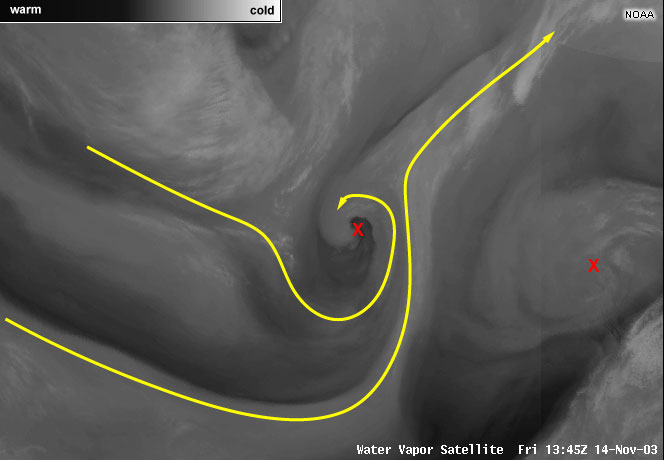
Here we have analyzed the most prominent vorticity maxima and axes of maximum winds. While watching the loop one can note the strong northwesterly (and lower altitude) flow that wraps into and around the vorticity maximum in the center of the image. The larger scale pattern to the east shows another axis of maximum winds, and a separate weaker and wider vorticity maximum.
Let's try another example. Follow the same process as in the previous question and check your analysis by clicking “done”.
Question 2 of 2


| Tool: | Tool Size: | Color: |
|---|---|---|
Again, we have strong northwesterly flow at mid-levels coming into a strong vorticity maximum in the center of the image. The brighter white region at the far west in image appears to be moving more directly to east than the main wind axis that is drawn in that location - one must remember that water vapor imagery shows many levels. The bright white is upper level moisture associated with air coming over the Rockies and is slightly higher in altitude than the northwesterly wind max.
Another main axis of winds lies in the southwesterly flow at bottom right of the image and is associated with the subtropical jet. Careful analysis reveals several other small-scale vorticity maxima in a chain along the axis of maximum winds coming into the cyclone at center, as well as two vorticity minima where there is anticyclonic motion.
Next we will look at the counterpart of vorticity maxima - the anticyclonic vorticity minima. They really are counterparts - where there is an axis of maximum winds, there must be a vort max on one side and a vort min on the other side somewhere along the line. Their strength, however, varies greatly upon scale and hemisphere, and orientation of shear and/or nearby circulation centers.
Pre-Lab: Identifying Vorticity Centers » Vorticity Minima Patterns
The shape of an anticyclonic anticomma pattern reveals the location of vorticity minima. The tabs below contain animations of a cloud area superimposed with rotation and shear, similar to those in the previous section. Again, X represents the total vorticity maximum, S represents shear, and R is rotational vorticity. Explore these common patterns of vorticity minima on satellite by clicking through the tabs and watching the animations.
Given pure rotation, the conceptual cloud line will evolve symmetrically. The vorticity minimum (N) is at the center of rotation, which is also the point of inflection. The rotational vorticity is the sole component of vorticity - there is no shear vorticity component.

Now we will add shear to the rotation. Winds are increasing to the south of the image center. Now, the point of inflection and total vorticity maximum are shifted toward the region of greater shear. The concave arc in the location of the wind maximum is enhanced. The convex arc to the north is unchanged, as it exists via the rotational component of the vorticity at the center of the circle.

If we increase the equatorward shear even more, the pattern becomes becomes more pronounced as below.

Finally, if the shear is on the poleward side of the rotation, the same shifting of the point of inflection/total vorticity maximum toward the region of shear occurs. In contrast, however, the convex arc in the location of the wind maximum is enhanced. The concave arc is not enhanced and is created purely by the rotational component of the vorticity, which remains unchanged and located at the center of the circle.

Pre-Lab: Identifying Vorticity Centers » Vorticity Minima Identification Practice
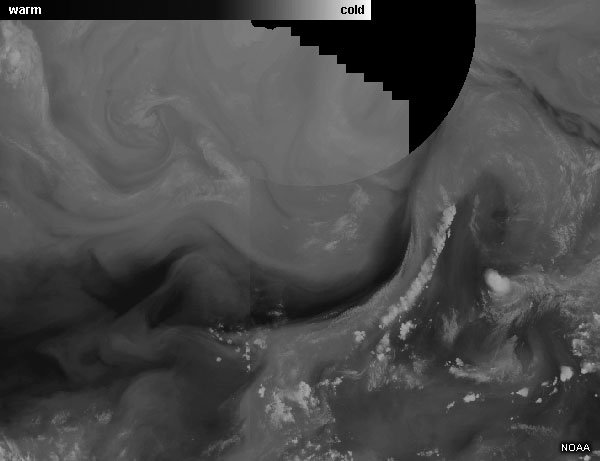
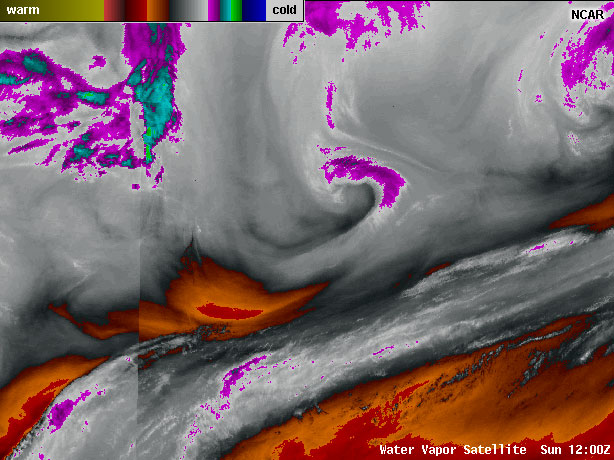
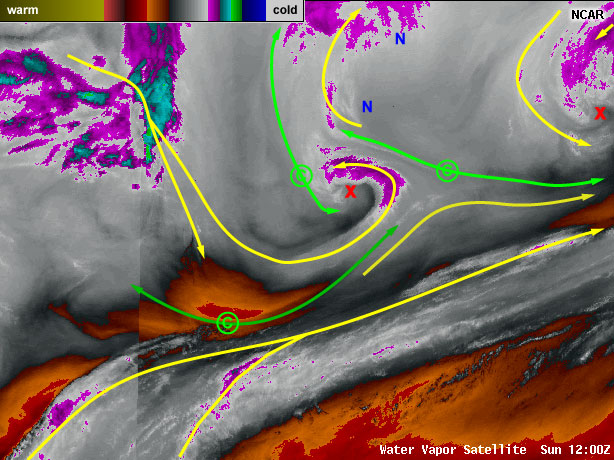
Now we will practice identifying both vorticity maxima and minima. Watch the loop in the first tab below. In the second tab, analyze the locations of the main vorticity maxima with a red dot and the main vorticity minima with a blue dot. Draw in a single axis of maximum winds using the yellow pen. Compare your answers to the solution by clicking “done”.
Question 1 of 2

| Tool: | Tool Size: | Color: |
|---|---|---|
There are a lot of waves and weak vorticity maxima that could be analyzed in this loop. For our purposes, the main vorticity maximum is noted with the red X. The main vorticity minimum is noted with the blue N, and lies to the south of where the main jet begins to curve anticyclonically.
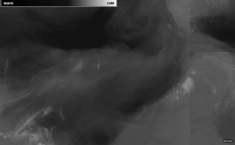
Let's try one more example. Analyze the vorticity centers and major axes of winds in the tabs below.
Question 2 of 2
| Tool: | Tool Size: | Color: |
|---|---|---|
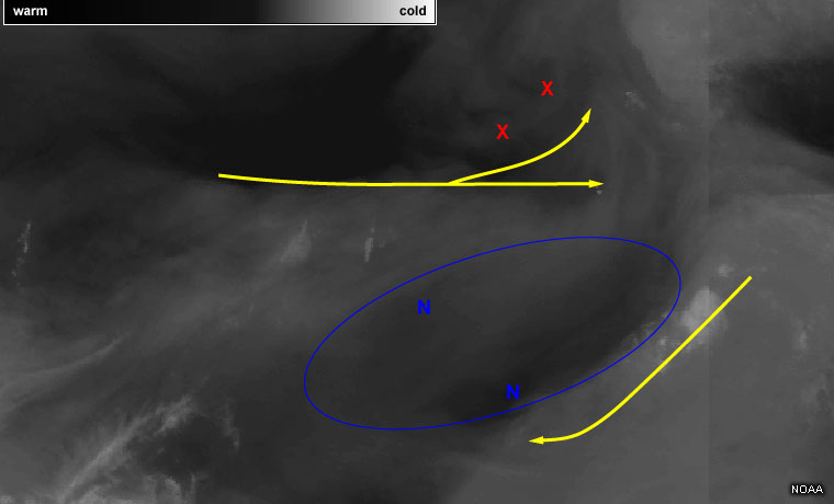
This case has a readily identifiable axis of maximum winds that is nearly zonal in the northern half of the image. There are a couple weak vorticity maxima along the northern side where cyclonic motion can be detected with the darker pulses.
The vorticity minima are noted with blue Ns. One could subjectively place the maxima at one of several locations where anticyclonic motion is most notable within the very broad clockwise flow (blue outline).
Now that you've had some practice with identifying vorticity centers and maximum wind axes, we will look briefly at how to identify the deformation zones around them using water vapor imagery.
Pre-Lab: Identifying Deformation Zones
A deformation zone is a region in the atmosphere with significant stretching or shearing. Spatial variations in the velocity field between two air masses cause a change in the shape of these air masses. Analysis of deformation zones is important in many situations since deformation is a primary factor in the processes of frontogenesis and frontolysis.

The dynamic features that best define a deformation zone on satellite are the associated vorticity maxima and minima that were discussed earlier. As shown below, a vorticity maximum and a vorticity minimum both straddle the inflow along the diffluent asymptotes, or axes of contraction, of a deformation zone. The incoming flow is then stretched out to both sides and forms the axis of dilatation, which is a confluent asymptote.
The relative strengths of X1, N1, X2 and N2 define the size, shape and movement of the deformation zone.

As illustrated in this conceptual view of a warm conveyor belt below, synoptic scale, quasi-horizontal motions are orders of magnitude larger than vertical motions in the atmosphere. This is the simple justification for drawing deformation zones on surfaces like isobaric charts while referring to the more detailed water vapor imagery to complete the visualization of current weather. This process can help students and forecasters develop a mental model of the atmosphere.

You will have a chance to combine knowledge in this way via analyzing temperature advection on pressure levels, deformation and vorticity on satellite water vapor loops, and surface streamlines for the same case during labs. For now, we’ll look at identifying common patterns of deformation before performing a larger scale deformation and vorticity analysis.
Pre-Lab: Identifying Deformation Zones » Common Deformation Zone Patterns
There are several common deformation patterns that occur on a regular basis in the atmosphere - we’ll look at four that focus on dominant vorticity maxima here. A representative satellite example of each deformation pattern is found after each description and conceptual model.
Pre-Lab: Identifying Deformation Zones » Common Deformation Zone Patterns » Straight Line
A straight line deformation zone with no wind maximum and no shear indicates the following:
- the confluent asymptotes are the same length
- vorticity centers are the same intensity
- moisture patterns are all the same size
- 2 comma and 2 anticomma clouds will mark the zone

Pre-Lab: Identifying Deformation Zones » Common Deformation Zone Patterns » Confluent Downstream
A straight line deformation zone with a downstream axis of maximum winds indicates the following:
- the downstream confluent asymptote will be longer
- the circulations paired across the confluent asymptote will be larger and created by both curvature and shear


Pre-Lab: Identifying Deformation Zones » Common Deformation Zone Patterns » Double Vorticity Maxima
When both confluent asymptotes of a deformation zone are curved cyclonically, the vorticity maxima pairs must be significantly more intense than the minima. A "backward S" deformation zone can be quickly sketched between the vorticity maxima as revealed by the large comma patterns.


Pre-Lab: Identifying Deformation Zones » Common Deformation Zone Patterns » Vorticity Maxima Chain
A chain of deformation zones can be quickly sketched between a series of vorticity maxima along a channeled jet. Subtle vorticity maxima can be analyzed at regular intervals, when the analyst detects a regular wavelength. This graphic illustrates how the "S" deformation zones between the vorticity minima relate to the "backward S" deformation zones between the vorticity maxima.


Pre-Lab: Identifying Deformation Zones » Deformation Zone Identification Practice
Now we will practice identifying and drawing deformation zones. Watch the satellite loops in the first tabs, and analyze major vorticity maxima, minima, axes of max winds, and deformation zones in the second tab. Click “done” to compare your analysis to the solution.
Question 1 of 2
| Tool: | Tool Size: | Color: |
|---|---|---|
We'll start our discussion with the southernmost axes of maximum winds - these are southwesterly flow associated with the subtropical jet.
The main player in the image is the vorticity maximum at the center of the page. This vort max/cyclone is on the north side of an axis of strong northwesterly flow. Note that this northwesterly jet is analyzed as split flow where part wraps around cyclone and part flows nearly due south. Air in this southward branch is also subsiding (sinking) to some degree.
At the point where the subsiding northwesterly flow spreads out in east and west directions (and also eventually cuts underneath moisture associated with subtropical jet), we can mark a deformation zone in green. This zone nicely aligns with the darkened filaments. The letter c denotes the "col" or neutral point.
Another deformation zone can be analyzed at the head of the strong flow that wraps around to the north and west of the vorticity maximum - as this wrap around encounters the background westerly flow, some of the flow will deform and stretch along the green axis.
A third deformation zone is evident as the some of the southwesterly flow coming just east of the cyclone wraps around to the west while the other portion begins to flow more easterly. The col is analyzed at the neutral point where the flow splits to west and east. This is a good real-world example of the warm conveyor belt animation that we watched in the deformation zone introduction!
We will try one more example before moving to the larger domain case in the lab.
Question 2 of 2


| Tool: | Tool Size: | Color: |
|---|---|---|
Again, we have a case with a pronounced cyclone/vorticity max near the center of the image. Strong northwesterly flow is splitting and wrapping around the cyclone while some is visibly turning the opposite direction (and subsiding to some degree). A green line denotes the deformation zone where the northwesterly flow stretches along a SSW-NNE axis. This lines up well with the dark filament in that location, and is trackable for many frames of the loop.
The main southerly flow that comes into the cyclone helps create two more deformation zones - one where the southerly flow splits between wrapping around the cyclone or heading to northeast (just like in the warm conveyor belt animation!), and another zone can be noted at the head of the wrap-around flow where the easterly winds meet the westerly background flow.
Finally, the northwesterly flow at the top of the image makes a classic deformation pattern as it nears the split of southerly flow into the cyclone. Another branch of strong northwesterly winds can be seen creating a deformation zone as some of the flow slowly subsides and spreads eastward and westward (note darkening and widening of red filament there in loop).
Next Steps: Lab Activity
A loop of GOES east water vapor imagery is available for analysis. This imagery is from the “continental US” case that is also analyzed in the streamlining and advection labs. You can download a zip file of the imagery below, and it is also available in the vorticity and deformation zones folder on the course site http://courses.comet.ucar.edu/course/view.php?id=165
The images are large enough to print well on 8.5” x 12” copy paper without resizing, or they can be imported to MS Powerpoint or other software that contains drawing capabilities. Analyze the image from 2030Z on March 2.
Consult your instructor for further details on format or other recommended analysis times.
ReferencesHahn, B. B., E. Rall, and D. W. Klinger, 2002: Cognitive analysis of the warning forecaster task. Klein Associates, Inc., Final Rep. RA1330-02-SE-0280, NOAA/NWS Office of Climate, Water, and Weather Services, 26 pp. [Available from Klein Associates, Inc., 1750 Commerce Center Blvd North, Fairborn, OH 45324-6362.]
Pliske, Rebecca M., Beth Crandall, and Gary Klein. "Competence in Weather Forecasting" Psychological Investigations of Competence in Decision Making, Ed. Kip Smith, James Shanteau, Paul Johnson, Cambridge University Press, 2004. 57. Print.
Stuart, Neil A., David M. Schultz, and Gary Klein. "Maintaining the role of humans in the forecast process." Bull. Amer. Meteor. Soc 88 (2007): 1893-1898.