BoM Aviation Fog Case
Fog Forecasting Supporting Topics
Table of Contents
- Case Reference Material
- Fog Theory
- Fog Formation and Dissipation Processes
- Forecasting
- Monitoring Tools
Selected COMET Modules with related information:
- Fog and Stratus Forecast Approaches
- https://www.meted.ucar.edu/training_module.php?id=149
- Forecasting Radiation Fog
- https://www.meted.ucar.edu/training_module.php?id=39
- Applying Diagnostic and Forecasting Tools
- https://www.meted.ucar.edu/training_module.php?id=117
Case Reference Material
Maps
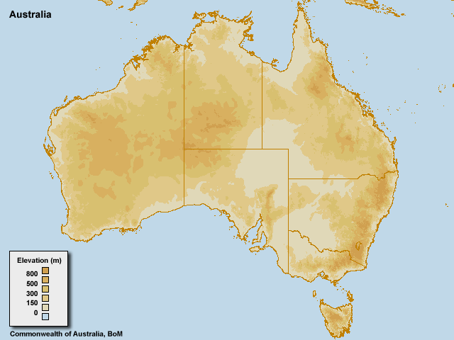
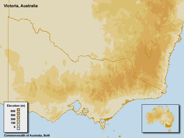
Local Geography and Influences
The setting for this case is Melbourne, Victoria, located in southeastern Australia. The Melbourne metropolitan region is home to 3.9 million people. The Great Dividing Range lies to the west, north and east of the metropolitan area. To the south of Melbourne is Port Phillip Bay, which opens out to Bass Strait, the body of water between mainland Australia and Tasmania.
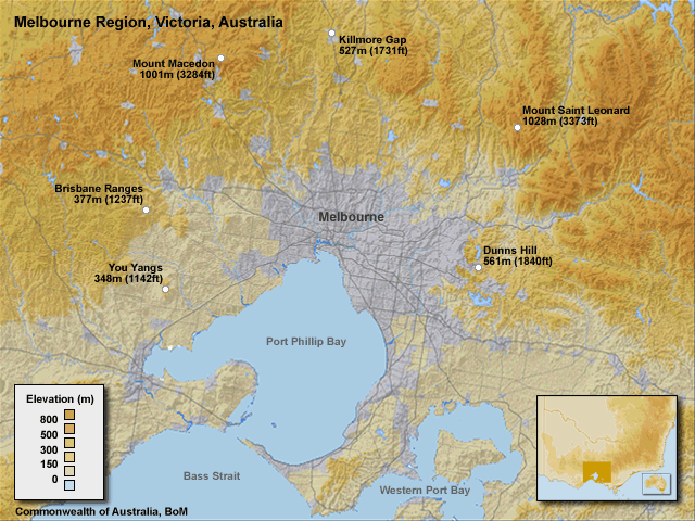
The highest elevation in the area surrounding Melbourne is to the east with Dunns Hill at 561m (1840ft), and further to the northeast Mount Saint Leonard at 1028m (3373ft). To the northwest of Melbourne is Mount Macedon, 1001m (3284ft ), and to the west there are several smaller ranges, the You Yangs, 348m (1142ft) and The Brisbane Ranges, at 377m (1237ft).
The location of the mountains of the Great Dividing Range can have a large influence on the local winds. In certain situations, they can act to block light southerly winds or they can be the source of night-time, northerly, katabatic, or drainage winds.
Port Phillip Bay and Bass Strait are other geographic features of importance, as they can provide a source of moisture with southerly winds. The sea surface temperature, which for this case is around 19°C in the Bay, can have an influence as well.
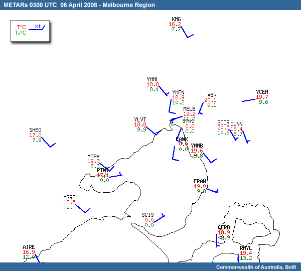
Local Airports and Elevations

Automated Weather Station (AWS) Elevations
| Station Name | Abbreviation | Elevation (m) |
|---|---|---|
| Melbourne/Essendon | YMEN | 78 |
| Viewbank | VBK | 66 |
| Coldstream | YCEM | 83 |
| Scoresby | SCOR | 80 |
| Frankston | FRAN | 6 |
| Cerberus | CERB | 13 |
| Rhyll | RHYL | 13 |
| South Channel Island | SCIS | 9 |
| Fawkner Beacon | FAWK | 0 |
| St. Kilda Harbor | STKI | 6 |
| Point Wilson | PTWI | 18 |
| Sheoaks | SHEO | 237 |
| Aireys Inlet | AIRE | 95 |
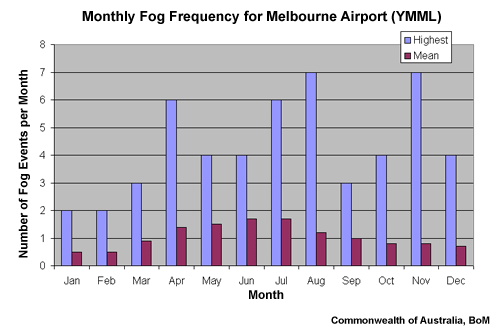
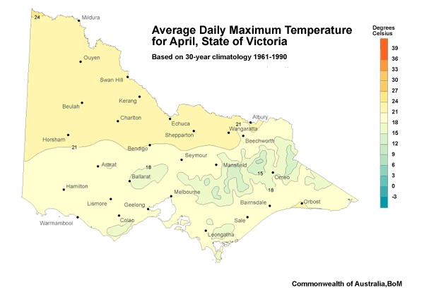
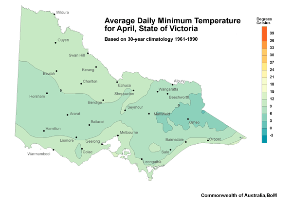
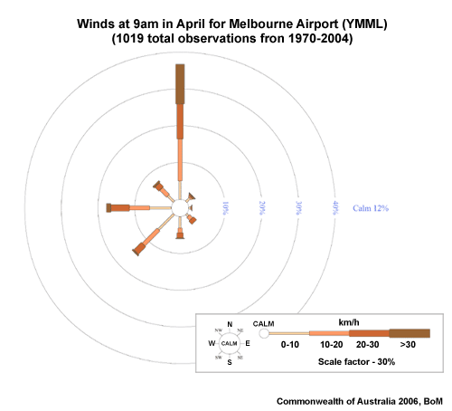
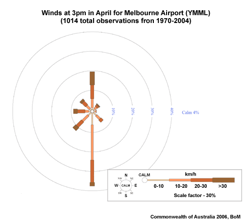
Local Climatology of Fog, Temperature and Wind
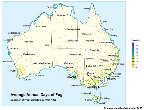
Fog has the potential to form almost anywhere in Australia, given the right conditions. This map shows the average number of days fog is observed at each marked location.
The following data is more specific to the Melbourne region and Melbourne Airport in particular.
Local Fog Aids
Local fog forecasting aids are used throughout Australia to help in the forecast decision process. These aids have been developed over the years by forecasters or researchers and vary greatly. They range in the different aspects they try to predict, from forecasting onset time or the duration or likelihood of fog. They also differ in terms of the types of weather parameters taken into consideration, such as pressure, moisture, and synoptic type. Each local fog aid uses a different calculation method ranging from a checklist approach to statistical regression.
A national fog forecasting aid was developed by Livio Regano, BoM, and is available for most TAF locations throughout Australia. The aid uses a statistical forecasting approach, recording the current values of a set of specially selected atmospheric parameters and searches the BoM climate database for past events with a similar set of values. The percentage of fog occurrences on these days can then be related to the real-time fog probability. Verification of the aid shows that it performs better the higher the number of similar events.
The Stern/Parkyn synoptic classification aid, assigns the current forecast synoptic situation into one of 50 different synoptic types. To determine the different synoptic type the aid takes into consideration the gradient wind strength, wind direction and the cyclonicity of the synoptic situation, using pressure values from six locations in southeastern Australia. A climatology of the likelihood of fog for each synoptic type has been produced based on the synoptic type.
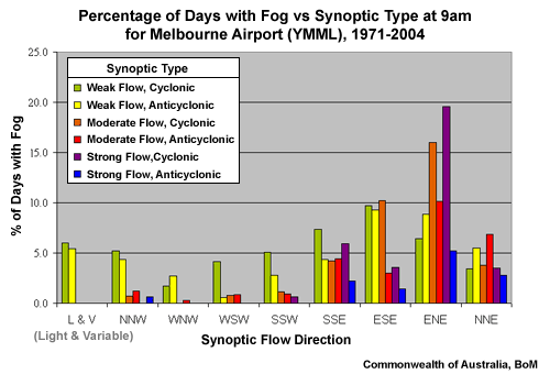
Once the synoptic situation is classified the aid uses logistic regression with the previous afternoon's dewpoint, temperature and time of year to determine a specific fog probability for the particular situation.
For more information, see the full paper linked here (.pdf).
In Victoria, a Bayesian Objective Fog Forecast Information Network (BOFFIN) has been developed, which combines several fog predictors, previous available guidance and operational forecasts. The previously developed aids are the Stern/Parkyn fog aid and Regano's aid (mentioned above). The new predictors identify the pressure gradient, moisture, rainfall, temperature lapse rate and time of year. The Bayesian network (BOFFIN) uses probability to combine predictors and previous guidance, to produce uncalibrated fog probabilities and ultimately fog forecasting decisions. It appropriately weights different pieces of information after assigning the probability of each state (eg. Very Favourable, Favourable, Unfavourable), ultimately resulting in a percentage likelihood of fog.
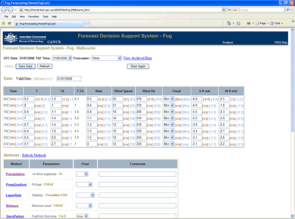
The Bureau of Meteorology's Research Division is developing and implementing nationally a generic web interface and national database for the local fog aids in the various states of Australia, called the Forecast Decision Support System (FDSS).
Local Procedures and Directives
As fog is a very localised phenomenon, each region has a set of local procedures which are set out in a local fog directive. Refer to your regional office's resources for more information.
Fog Theory
Definition of Fog
Fog is a suspension of very small, usually microscopic water droplets in the air, reducing visibility at the Earth's surface. The visibility shall be less than 1000 metres (fog), or at least 1000 metres but no more than 5000 metres (mist) (WMO No.306 and WMO No.407).
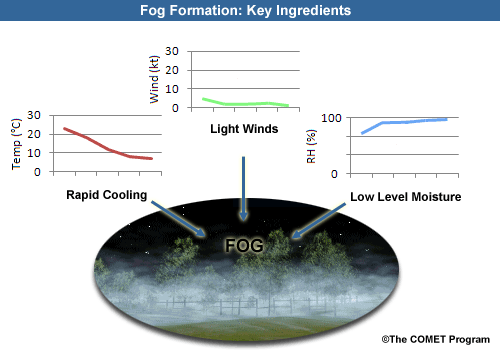
The development of fog requires all key ingredients to coincide at the same time. The key ingredients are rapid cooling in atmospheric layers immediately adjacent to the surface, sufficient moisture and light winds.
Types of Fog
Radiation Fog
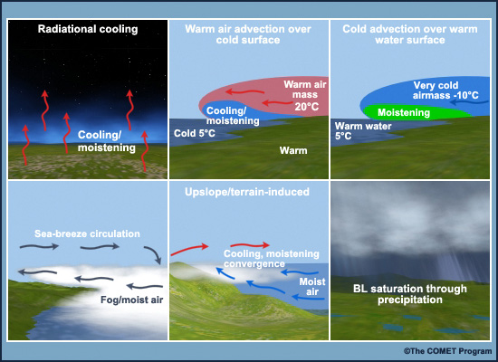
Radiation fog is created when radiational cooling at the earth's surface lowers the temperature of the air near the ground so that saturation occurs. Formation is best when there is a shallow surface layer of relatively moist air beneath a drier layer, clear skies, and light surface winds. This occurs primarily during the night or early morning.
This type of fog forms and completes its life cycle in situ. Boundary layer dynamics and adiabatic processes are negligible. Associated wind speeds are generally 5 knots or less. Stronger winds are generally detrimental to radiation fogs. Greater turbulent mixing entrains dry air layers from above into the fog layer.
Advection Fog
Advection fog can result from various scenarios. In the situation where warm air advects over a colder water surface, the warmer air cools down to its dewpoint causing fog to form. Some moisture may also be introduced into the air mass in the lower levels, but the main process at work is cooling of the air mass to saturation through conduction and light turbulent mixing. This type of advection fog is commonly referred to as sea fog.
Advection fog can also form in the opposite scenario, when cold air advects over a warm water surface. As the cold air moves over the water surface, water evaporates into the air mass, increases the near-surface moisture content resulting in fog formation in the lower levels. This type of advection fog is commonly referred to as steam or evaporation fog.
This type of fog forms primarily through boundary layer dynamic and adiabatic processes, and is dominated by synoptic-scale processes that affect the lifetime of the event. Radiative processes still play a role in its development and life cycle, but are not dominant. Formation can occur with light to moderate winds in the low levels.
Upslope/Terrain Induced Fog
Another fog or low-stratus forming mechanism is associated with the development of upslope or terrain-induced flow. As moist air is forced upslope, it cools adiabatically and saturation may result.
Rain/Post-Frontal Fog
When precipitation falls through dry air the liquid drops or ice crystals evaporate or sublimate directly into water vapour. The water vapour increases the moisture content of the sub-cloud layer while cooling the air. Fog can form as a direct result of precipitation falling through the boundary layer, or subsequently due to the increase in the amount of moisture within the boundary layer from the precipitation to precondition the atmosphere for fog, so that fog can form once the associated precipitating clouds clear and overnight cooling ensues.
Blocked Flow Fog/Stratus
Cool moist "on-range" flow may be blocked by a mountain range if the flow speed (kinetic energy) is not great enough to lift air parcels upslope against the affects of negative buoyancy. The upslope ascent initiates saturation on the slopes of the mountain.
Valley Fog
Valley fog forms when air near the terrain height cools, usually by radiation at night. As the air cools it becomes denser than its surrounding and sinks towards the centre of the valley. This results in the creation of a pool of cold air at the valley floor. If the air is cold enough to reach its dewpoint temperature, fog formation occurs.
Advected Fog
Advected fog is fog that has formed in one place and is transported elsewhere. It is different from advection fog which is characterised by turbulent fluxes of heat and moisture between the surface and adjacent atmospheric layers as the air-mass advects across the surface.
Fog Formation and Dissipation Processes
There are four parts to address the life cycle of a fog event:
- Preconditions
- Formation and Growth
- Maintenance
- Dissipation
Preconditions
Fog cannot form unless the
necessary conditions and key ingredients coincide. To form any type of
fog or low stratus in the boundary layer, the temperature and dewpoint must
approach each other. This can occur by either increasing the amount of moisture
in the boundary layer or decreasing the temperature in order to achieve a saturated
state. The processes by which saturation occurs distinguish the type of fog or
stratus event that is occurring.
Regardless of the process, a common characteristic of a fog scenario includes an inversion. Without an inversion to trap moisture, the drier layers of the atmosphere just above the moist layer will mix in, and the entrained drier air will cause any fog or stratus that has developed to mix out and dissipate. In order to develop a sustained fog or stratus event, an inversion with associated decoupling of the boundary layer from the atmosphere above it, is a prerequisite.
Radiational processes typically have an influence in the formation of most fog events. Therefore we will concentrate on radiational processes.
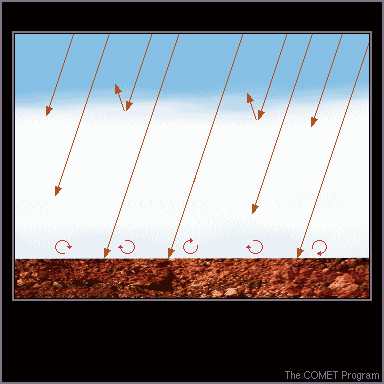
The key low-level ingredients required to generate a radiation fog are moisture, rapid cooling of atmospheric layers adjacent to the surface, and calm or light winds. As surface long-wave energy is radiated into space, the ground surface cools rapidly and induces cooling of the lowest few meters of the atmosphere, creating a shallow surface-based inversion. If there is enough water vapor in the near-surface atmospheric layers and enough cooling, the low-level air eventually reaches saturation.
The amount of radiative cooling of the surface also depends upon the amount of cloud covering the sky. Overcast skies can trap 90% of the radiation emitted by the earth. Dry air aloft enhances radiative cooling at the surface. Low-level anticyclones can create favorable conditions for radiation fog by suppressing surface winds and drying the air aloft through subsidence.
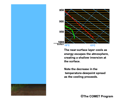
When afternoon temperatures are cool prior to nightfall, the time required to reach saturation on a clear night is shortened.
Cooling of the lowest layers causes the layer to become increasingly stable and resistant to weak turbulent mixing near the surface. Eventually the weak turbulent mixing may cease altogether and together with continued cooling, allows excess water vapour in the layer just above the surface to condense into fog droplets.
Formation and Growth
Radiative cooling may progress to the point where the air just above the ground becomes supersaturated and fog droplets form by condensation.
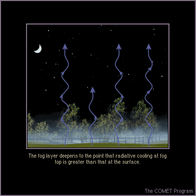
During the initial stage of fog formation, cooling continues at and near the surface until the fog depth reaches several meters, deep enough to begin to absorb and reemit radiation originating from the earth. This slows the rate of cooling at the surface, and the fog top becomes the level at which radiative cooling and condensation processes are most active.
Maintenance
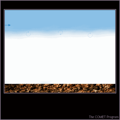
During the maintenance phase, a significant fog layer maintains a relatively constant depth. This phase is characterized by a balance between opposing forces. These forces are fog-top radiative cooling, droplet settling, and fog-top mixing.
Fog-top condensation balances evaporation and droplet settling processes to maintain the depth of the fog layer. Radiative cooling at fog top replenishes the supply of droplets as they settle downward, and even tries to strengthen the inversion and deepen the fog. At the same time, turbulent mixing attempts to weaken the inversion and erode the fog top. Since winds generally increase with height, a radiation fog layer typically deepens during its growth phase until it reaches a height where the winds are strong enough and induce enough fog-top mixing to halt the growth.
Introduction of mid- and upper-level cloud layers, during the daytime, can help to maintain the radiation fog layer. These clouds reduce the solar radiation received at the ground surface, preventing warming at the surface and maintaining a higher relative humidity in the lower portions of the fog layer.
However, the lower the level of an overlying cloud layer, the more it can reduce radiative cooling and condensate production at fog top, allowing dissipative processes such as settling to take over.

Dissipation
The duration of the dissipation phase can vary due to several factors. Dissipation of droplets is generally caused by one or more of the following processes:
Solar Radiation
During the daytime, solar radiation is absorbed by the ground, even when there is an intervening layer of fog. As the ground warms, it heats a thin skin of air in contact with the surface through conduction. This heat initiates weak convective mixing, which begins to warm the lowest portion of the fog layer. The relative humidity in this layer begins to decrease, slowing the formation of fog droplets and eventually evaporating existing droplets. As the fog thins, the warming process accelerates, allowing more solar radiation to reach the ground. With moderately strong sunshine, the base of a fog or low cloud layer can lift at a rate of up to several hundred feet per hour.
Droplet Settling
Regardless of their size, all fog droplets continually settle. The depth of a fog layer decreases when the droplet formation rate cannot keep up with the settling rate. An average fog droplet, which is less than 20 micrometers in diameter, will settle at the rate of 1 cm/sec. So, fog initially 30 meters (or about 100 feet) deep should settle to the ground in about an hour if the maintenance processes are removed.
Wind Shear/Turbulent Mixing
A fog layer's capping inversion is often accompanied by a layer of significant vertical wind shear. Turbulent mixing of warmer and drier air into the top of the fog layer can reduce relative humidity in that layer and lower the inversion. The weaker the capping inversion is, the more susceptible it is to this ongoing mixing and erosion process.
Changes in the Wind
Introduction of moderate to strong low-level winds can cause fog to dissipate both at the fog top and near the surface. At the fog top, winds entrain warmer, drier air from aloft into the fog. Near the surface, winds cause mixing of the surface-warmed air with the fog above. Both promote evaporation of fog droplets and improved visibility.
Overlying Cloud Layers at Night
At night, loss of radiant heat is most rapid when there are no clouds above an established fog layer. If a broken or overcast layer of mid-level or a thick layer of upper-level clouds is introduced, fog-top cooling decreases because less radiation is able to escape the atmosphere. This effect can slow the rate of new droplet formation and contribute to fog dissipation.
Forecasting
Fog is a difficult phenomenon to forecast. For fog to form, all the key ingredients need to coincide. Slight deviations from the expected conditions, can be enough for the formation not to occur,
Forecasting fog is typically a short term forecast or 'nowcast'. Local influences can dominate the likelihood of fog formation. The key to fog forecasting is having a good understanding of the current environment and then a good handle on the expected evolution of the situation in the coming 24 hours.
Identifying Precursors
Understanding and being able to identify the precursors to fog formation is the key to providing a longer lead time for the users of your forecast product. Having awareness of typical synoptic weather systems that are more likely to produce fog conditions, can provide an alert to forecasters days ahead of the event. The most common synoptic situation for fog formation is a surface high pressure system, as they typically promote the key ingredients required; rapid cooling, moisture and light winds. Once this situation is evident it is necessary to confirm whether the key ingredients are in fact sufficient and coincident. Combining current observations with forecasting tools (eg. NWP, local aids) provides a comprehensive way to identify the precursors.
Forecasting Tools
NWP
While models typically do not accurately diagnose fog, they are useful for examining the atmosphere's dynamics, mass balances, and moisture. Keep the following model weaknesses in mind with regard to assessing fog potential:
- Poor to fair moisture depiction, especially in the lower boundary layer
- Incomplete boundary layer physics
- Insufficient resolution of surface and boundary layer processes
- Insufficient resolution of surface characteristics such as vegetation, soil type/moisture, terrain, etc.
While models often fail to depict the meso- and local-scale processes that are critical to fog and stratus development, they often do well in depicting the larger picture. Standard model plan views and cross-section data can provide valuable synoptic information on expected pattern development that may aid or inhibit fog or stratus development. Some of the more common combinations that can be useful in fog/stratus forecasting are:
Plan Views:
- Relative humidity at all levels
- Low-level winds
- Vertical velocity aloft
- Height fields
- Sea-level pressure
- Moisture and temperature advection
Cross Sections:
- Relative humidity
- Vertical motion
Model Soundings
While model soundings provide the same basic information as observed soundings, they offer the following additional advantages:
- Spatial: Available at many more locations
- Temporal: Updated every model run, which can vary from every 3 to 6 hours
- Forecasts of future conditions from every 1 to 6 hours and to several days out, depending on the model
Ground Truthing/Verification
While NWP guidance is a useful tool in forecasting, the performance of the model should ALWAYS be verified against observational data. If the model is not performing well at the analysis or short-term forecast time steps, then caution should be taken when using the longer lead-time model forecasts. Ground truthing involves assessing the performance of the model at a particular time over a spatial extent.
For example, a quick comparison of the model analysis of MSLP, height and moisture fields to surface observations and satellite imagery can be used to verify the model placement of ridges, troughs, pressure systems and associated cloud features. Adjusting for any discrepancies is an important task in any forecast process but especially so for fog since subtle environmental changes can have an impact on the presence of key fog ingredients.
Local Fog Aids
Local fog aids can provide the forecaster with statistical approaches to the likelihood of fog. These are a great tool to help with your decision making, but the limitations of the aid should always be taken into account. Forecasting aids should never be used blindly in isolation, but in a manner that enhances your own forecasting skills being utilised in the context of all observations, data and conceptual models. The specifics on local fog aids for the region are available under the References section.
Forecasting Methods
Two of the most useful forecast methods for forecasting fog are climatology and persistence methods. Climatology provides a statistical insight into past events at that location. Some climatologies are more detailed than others, ranging from likely occurrence of fog for that particular time of the year, to likelihood of fog for given values of weather parameters, eg. synoptic flow, dewpoint temperature. This allows you to quickly compare your current situation with other situations when fog has occurred.
Persistence forecasting is commonly used when the weather situation has not changed significantly from the previous day. This often occurs with potential fog events being associated with very slow-moving, dominant high pressure systems in the region. Starting with the conditions that have occurred in the past 24 hours, query what has and will change that will prevent fog conditions from occurring again? Did fog occur last night? What would stop fog from forming again this evening? Cloud? Wind strength? Wind direction? Moisture amounts? If fog didn't occur last night, what may change that would provide more favourable conditions for fog to develop tonight.
Fog Type/Classification
Understanding the type of fog that is expected to develop will help with detecting the conditions for fog formation and focusing on key parameters and data. For example, imagine a scenario whereby a forecaster is expecting radiation fog to form and currently observed light winds are expected to prevail overnight. The main forecast consideration in this situation might relate to whether the surface layers will reach saturation overnight. In this scenario the forecaster, may keep a particularly close eye on temperature trends, or the advection of moisture. See Fog Types for details on specific fog types.
Forecast Products
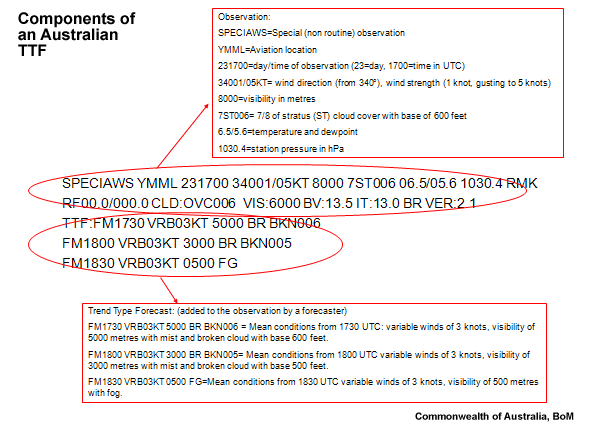
Two of the routine aviation products issued by the Australian Bureau of Meteorology featured in this case study are the Terminal Aerodrome Forecast (TAF) and Trend Type Forecast (TTF). TAFs are issued for hundreds of airports around Australia. They range from 6 to 30 hour validity, depending on the frequency of traffic at the airport. The TTF is a 3 hour product issued at around 18 of the major airports in Australia.
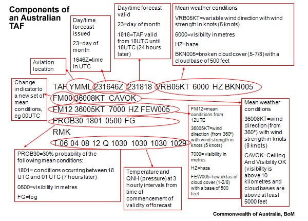
TAF Example
        TAF YMML 231646Z 231818
        VRB05KT 6000 HZ BKN005
        FM00 36008KT CAVOK
        FM12 36005KT 7000 HZ FEW005
        PROB30 1801 0500 FG
        RMK
        T 06 04 08 12 Q 1030 1030 1030 1029
TTF Example
        SPECIAWS YMML 231700 34001/05KT 8000 7ST006 06.5/05.6 1030.4 RMK
        RF00.0/000.0 CLD:OVC006 VIS:6000 BV:13.5 IT:13.0 BR VER:2.1
        TTF:FM1730 VRB03KT 5000 BR BKN006
        FM1800 VRB03KT 3000 BR BKN005
        FM1830 VRB03KT 0500 FG
Monitoring Tools
Satellite Imagery
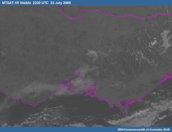
Satellite imagery is one of the most useful tools to a fog forecaster. The key advantage of satellite imagery over other observational tools, is it provides a vast spatial extent of coverage for identifying and/or monitoring fog. Often the timing of stratus or fog moving in or out of a location, dissipating or forming can be assessed by viewing loops of visible, IR, and fog product imagery. The imagery can show where fog or stratus is eroding or spreading and can be used to identify synoptic and mesoscale features. Infrared imagery is also useful for monitoring mid- and high-level clouds to anticipate their effects on underlying stratus and fog. For example, the presence of high clouds during the daytime can hinder heating and the subsequent dissipation of low stratus or fog.
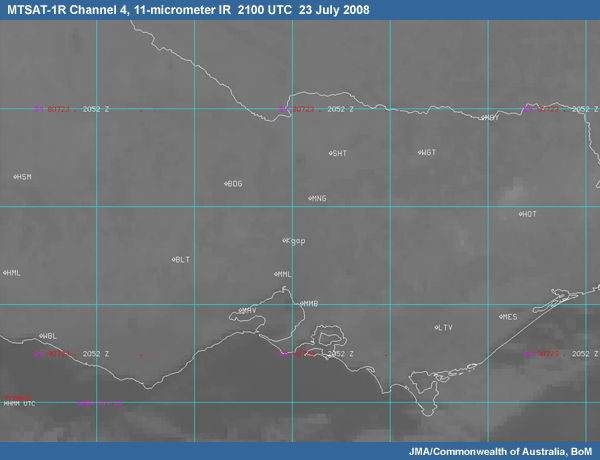
11-micrometer Longwave and 3.7-micrometer Shortwave IR Channels
The 11-micrometer IR "window" channel is used for all-purpose cloud detection at night. The 11 micron channel (detecting long-wave radiation from emitting surfaces like cloud-tops) can be used for cloud-top height estimations and can be used to detect surface temperature patterns associated with areas of higher surface moisture (and dew points). Note the darker gray areas indicating low clouds or fog in the image.
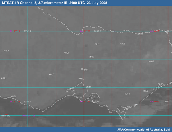
The 3.7-micrometer channel (channel 3) is also an IR window channel that is even more transparent to moisture than the 11-micrometer band. Even when used alone, imagery in this channel can show surface temperature variations and the edges of low clouds and fog much better than the 11 micron channel.
Fog/Low Cloud Product (3.7-11 micrometers)
The physical properties of fog and low cloud allow them to be distinguished from other clouds by way of their ability to absorb and reflect electromagnetic waves, and in particular infrared radiation (IR). The satellite fog product outlined here utilizes a channel differencing methodology. It takes advantage of the emissivity properties of infrared radiation waves. Opaque clouds composed of small water droplets have a higher emissivity at 11 micrometres than at 3.7-micrometers. Therefore there are differences in the brightness values between the 11 and 3.7 micron channels when these two spectral windows are compared.
The difference product (3.9-10.7-micrometers) corresponding to the previous two infrared images is shown below. Note how the fog stands out much more clearly in the difference product than in either the 3.9 or 10.7-micrometer products individually.
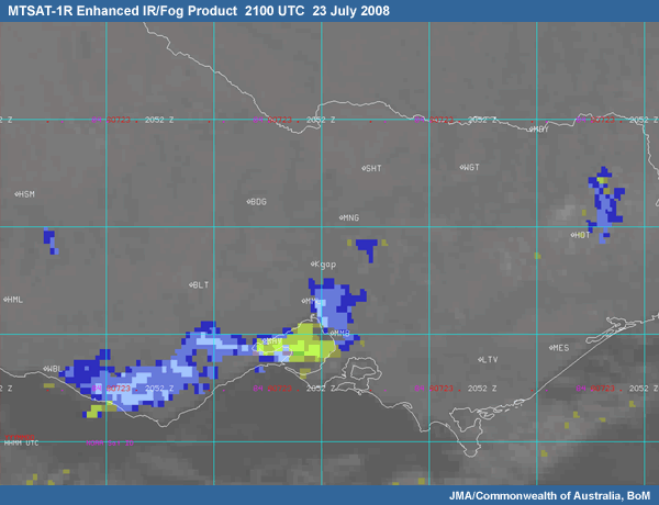
The fog/low cloud product or enhanced IR image algorithm checks cloud top heights by reference to nearby infrared radiation image pixels. If a cloud pixel is "cold" compared to nearby pixels, the radiating surface (cloud top) corresponding to that pixel is likely to be above the ground. If a cloud pixel (temperature) cannot be easily distinguished from nearby pixels, the effective cloud top is likely to be on or near the ground. The approach is conservative and genuinely low cloud pixels are rarely discarded.
Clouds coloured grey-blue (weak detections) through to light blue and red (strong detections) have tops not significantly cooler than nearby pixels. So they are more likely to be close to or on the ground.
Clouds coloured brown (weak detections) through to green (strong detections) have tops at least 4.5 K cooler than nearby pixels. So they are at least 500m above the ground in most cases — depending on atmospheric structure. However, fog may occur underneath such pixels.
Night-time thin cirrus is shown in pink where detected.
Uncoloured clouds have tops at least 9 K cooler than nearby pixels. So they are at least 900m above the ground in most cases. However, again fog may occur underneath.
Pixels at cloud edges may be contaminated and appear warm due to the cloud being thin, or more likely only partially filling a pixel (a warm background forms part of the pixel). This means pixels at the edge of a cloud may be designated as fog or low cloud (hence coloured) even though the bulk of the cloud is clearly cold.
False weak detections are common in desert areas. In these areas, you may wish to presume 'no fog/low cloud' unless moderate detections or low dewpoint depressions are found.
Fog/very low cloud is not the only water cloud to contain small droplets, and so false detections can occur. In particular, 'low' stratus-like cloud (including some stratocumulus) is often associated with limited turbulence, where the growth of droplets by collision is reduced. The fog/low cloud algorithm often colours these clouds even when their tops are clearly above ground. The conditions in which these clouds form are often also conducive to drizzle (hence productions of low cloud and/or fog beneath) and/or moist near-surface air under an inversion. Small droplets and false detections can occur in wave (lenticular) cloud, presumably because of the limited lifetime of the droplets therein and their limited opportunities to collide to form bigger droplets.
Visible Channel
This band shows reflected visible energy from clouds and surface features. Fog and low stratus appear relatively bright in visible images because of small cloud droplet diameters, although not as bright as thunderstorms, due to their relatively shallow thickness. Visible images are used to monitor fog dissipation as the sun heats the earth's surface.
METARS
Surface observations are very useful in diagnosing trends based on current and past conditions. Parameters such as winds, temperatures, dewpoints, sky conditions, clouds, weather, and visibility all provide valuable clues to potential fog or stratus development.
        METARAWS YMML 020700 16007/08KT CAVOK 11.8/07.0 1026.0
        METARAWS YMML 020730 15007/09KT CAVOK 10.9/07.1 1026.3
        METARAWS YMML 020800 14005/07KT CAVOK 11.2/07.0 1026.5
        METARAWS YMML 020830 14005/06KT CAVOK 11.3/07.1 1026.7
        METARAWS YMML 020900 05004/05KT CAVOK 10.2/06.8 1027.0
        METARAWS YMML 020930 00000/00KT CAVOK 10.7/06.7 1027.2
        METARAWS YMML 021000 36003/05KT CAVOK 08.0/06.1 1027.6
        METARAWS YMML 021030 36005/06KT CAVOK 09.8/06.8 1027.6
        METARAWS YMML 021100 35006/07KT CAVOK 07.1/05.8 1027.9
        METARAWS YMML 021130 33002/04KT CAVOK 07.4/05.9 1027.9
        METARAWS YMML 021200 35005/06KT CAVOK 07.7/06.0 1027.8
        METARAWS YMML 021230 35007/08KT CAVOK 07.1/05.3 1027.8
        METARAWS YMML 021300 34004/06KT CAVOK 06.2/05.3 1027.7
        METARAWS YMML 021330 35005/06KT CAVOK 06.0/04.7 1027.5
        METARAWS YMML 021400 36006/07KT CAVOK 05.5/04.8 1027.4
        METARAWS YMML 021430 35007/09KT CAVOK 05.3/04.6 1027.4
        METARAWS YMML 021500 34001/05KT 9000 SKC 04.4/04.0 1027.1
        METARAWS YMML 021530 35005/06KT 8000 SKC 04.7/04.2 1027.2
        METARAWS YMML 021600 36004/05KT 8000 1ST005 04.6/03.9 1027.4
        METARAWS YMML 021630 36003/04KT 8000 VCFG 1ST004 06.1/05.4 1027.4
        METARAWS YMML 021700 00000/00KT 8000 VCFG 3ST003 03.7/03.2 1027.5
        SPECIAWS YMML 021716 00000/00KT 5000 BR 5ST003 04.3/03.8 1027.4
        SPECIAWS YMML 021730 31004/05KT 5000 BR 7ST001 05.7/05.3 1027.4
        SPECIAWS YMML 021749 30005/05KT 3000 BR 8ST001 07.1/06.7 1027.2
        SPECIAWS YMML 021749 30005/05KT 3000 BCFG 8ST001 07.1/06.7 1027.2
        SPECIAWS YMML 021800 31004/04KT 3000 PRFG 8SC001 07.2/06.7 1027.1
        SPECIAWS YMML 021814 31002/04KT 0900 FG 8ST001 06.4/06.2 1027.1
        SPECIAWS YMML 021830 32003/05KT 0200 FG 8ST001 06.7/06.7 1027.1
        SPECIAWS YMML 021900 00000/00KT 0100 FG 8ST001 06.7/06.5 1027.1
        SPECIAWS YMML 021930 00000/00KT 0100 FG 8ST001 07.0/07.0 1027.4
        SPECIAWS YMML 022000 28004/06KT 0100 FG 8ST001 06.8/06.8 1027.6
This sequence shown here are surface observations just prior to and during a fog event. The observations indicate several factors conducive to fog development:
- Weak surface winds
- Small and decreasing dewpoint depression with time
- Mist prior to fog development
- Wind direction trends, which can be particularly important when flow source regions (such as water bodies) or locally induced terrain flows need to be carefully monitored.
Surface observations and trends are an important tool to use in the forecast process. For fog and low stratus, be aware of the trends in the following observed parameters:
- Temperature/dewpoint and dewpoint depression
- Cloud heights, coverage, and types
- Past and present weather
- Visibility
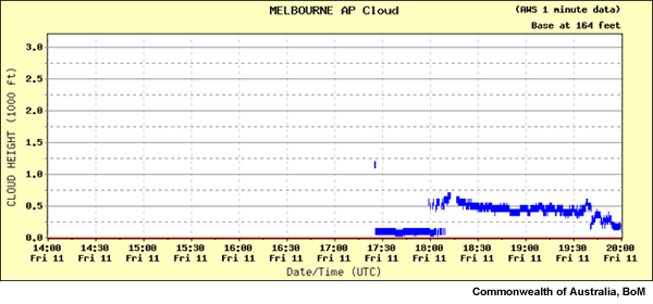
Ceilometer/Visibility Meters
Ceilometer
Laser ceilometers employ a laser light source to send a light pulse vertically through the atmosphere. The light pulse is scattered by aerosols including water droplets and the component of light scattered back towards the ceilometer is measured at the receiver. The height of the scattering obstruction is proportional to the time taken for the signal to return. A profile of return signal strength versus height is thus constructed and analysed to determine cloud base heights. They provide reliable determination of cloud height up to 12,500 feet.
To estimate cloud amounts an algorithm is used to process measurements collected over a period of time. If the cloud is evenly distributed perpendicular to the wind direction and only slowly developing or dissipating, the algorithm can give a good picture of the cloud downstream from the ceilometer. In many cases this is a reasonable assumption.
The Sky Condition Algorithm used by the Bureau of Meteorology uses cloud height reports up to 12500 feet collected over a 30 minute period. Data collected in the last 10 minutes is given a double weighting to improve the response time changing conditions.
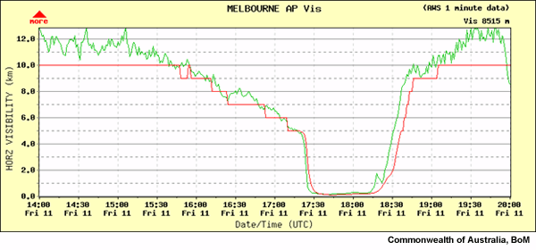
Visibility Meter
Visibility sensors evaluate the Meteorological Optical Range (MOR) by measuring the scatter of infrared light in air.
Forward scatter meters are the most commonly used visibility meter, in which the transmitter and receiver are located on two arms of a single unit, with the arms positioned to form an angle. The transmitter beams light into the air between the arms. Particles in the air cause the incident light to scatter and the portion of the signal scattered forward towards the receiver is measured by the receiver photodiode. Scattering due to water, dust, sand or smoke increases with the number of particles and hence with decreasing visibility.
If the visibility meter is appropriately sited and well maintained, it can provide useful guidance in the absence of a human observer; however the information should be used with care as it is sampling only 1 litre of air.
Differences in Instrument Data and Human Observations
Both are estimates of the current state of the sky and the visibility at the location. In essence;
- Automated sensors produce an estimate based on the continuous sampling of a single point over a period of time (30 minutes for the ceilometer, 10 minutes for the visibility meter).
- Human observers produce their estimate based on a view of the whole area and the whole sky over a relatively short time just prior to the observation.
Some limitations and advantages of the instrumentation
Advantages:
- Improved night observations — instrumentation has been shown to out-perform human observers at night.
- Consistent observations — unlike humans, the instruments provide consistent observations, site to site, day and night.
Limitations:
- Time lag — in rapidly changing situations the instrumentation will lag behind the actual situation. Human observers provide a snapshot at the time of the observation or may even anticipate changes and hold off the observation for a short time to be able to report significant developments.
- Misreporting stationary phenomena — ceilometers may under or over-report the amount of cloud when the cloud is stationary or the visibility meter may not detect stationary localized fog patches for long periods of time.
Soundings
Sounding profiles provide a wealth of information for diagnosing and forecasting fog and stratus. Observed soundings provide the best snapshot of the vertical structure of the atmosphere. Valuable information that can be gleaned from a local sounding includes:
- Location and strength of stable and unstable layers
- Temperature and dewpoint structure
- Inversion layers and strength
- Moist and dry layers
- Wind structure
- Potential for lifting or sinking motions
- Level at which clouds will form
- Indication of whether clouds will be stratiform or convective in nature
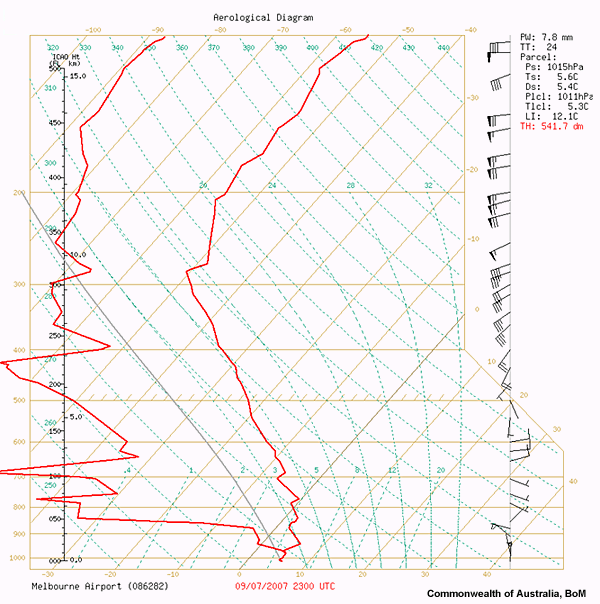
This sounding was observed when fog was observed and is a good example of a radiation fog profile. It shows a strong low-level inversion and a shallow saturated layer. These are features often associated with the formation/maintenance stage of radiation fog. Above the saturated layer, the temperature and dewpoint diverge to a difference of around 5°C, before quickly diverging to a difference of 30°C just above this. This "goalpost-shaped" sounding is typical of many radiation fog events. Winds reported within the fog are light, at or below 5 knots.
Limitations of observed soundings fall into three primary categories:
- Spatial: they are widely scattered and of insufficient density to always be of use, especially for local events
- Temporal: They are taken at most only once every twelve hours, which is typically insufficient to catch important changes in the atmosphere
- Resolution: The vertical resolution is often insufficient to identify subtleties that may be important to fog/stratus formation or dissipation